


Abstract
Quantum vacuum fluctuations are a direct manifestation of Heisenberg's uncertainty principle. The dynamical Casimir effect (DCE) allows for the observation of these vacuum fluctuations by turning them into real, observable photons. However, the observation of this effect in a cavity QED experiment would require the rapid variation of the length of a cavity with relativistic velocities, a daunting challenge. Here, we propose a quantum simulation of the DCE using an ion chain confined in a segmented ion trap. We derive a discrete model that enables us to map the dynamics of the multimode radiation field inside a variable-length cavity to radial phonons of the ion crystal. We perform a numerical study comparing the ion-chain quantum simulation under realistic experimental parameters to an ideal Fabry–Perot cavity, demonstrating the viability of the mapping. The proposed quantum simulator, therefore, allows for probing the photon (respectively phonon) production caused by the DCE on the single photon level.

Original content from this work may be used under the terms of the Creative Commons Attribution 3.0 licence. Any further distribution of this work must maintain attribution to the author(s) and the title of the work, journal citation and DOI.
1. Introduction
Vacuum fluctuations lie at the heart of quantum mechanics and quantum field theory, and many interesting physical phenomena are directly connected to virtual photons of the vacuum, like for example the Lamb shift [1] or the Casimir effect [2]. The dynamical Casimir effect (DCE) [3], which is related to the Unruh effect and the Hawking radiation [4], offers the possibility to turn these virtual photons into real measurable photons by moving the boundaries of a cavity with relativistic velocities and high accelerations (see figure 1(a)). Such extreme velocities, however, make it difficult to observe the DCE in a cavity QED experiment. Several proposals have been made to overcome this problem [5], for example, by replacing the moving mirrors by a rapid modulation of the electrical properties of the medium inside the cavity. One proposal, based on superconducting circuits [6, 7], has been implemented recently [8–10]. However, in that architecture it remains a challenge to analyze the generated microwave radiation on the single photon level [6].
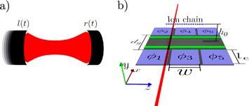
Figure 1. Setup. (a) Dynamical Casimir effect. Modulating the positions of the left or the right mirror of a cavity ( and r(t), respectively) results in the production of photons. (b) Proposed ion-trap-based quantum simulation. The dynamics of the radiation field inside the cavity is mapped to phonon modes of a chain of ions in a spatially dependent trapping potential, which can be engineered in a segmented surface trap. The modulation of the mirror is simulated via a laser field creating a time-dependent optical trapping potential (red line in x-direction). The example shows 6 DC electrodes (blue) and two RF electrodes (green). The distance between the DC electrodes is denoted , their length (both along the x-axis), and their width along the z-axis w. The ion chain (blue dots) is trapped at the center of the trap at the height h0 above the surface.


Download figure:
Standard image High-resolution imageIn this article, we investigate the possibility to implement a quantum simulation of the DCE by using an ion chain confined in a segmented surface trap [11], as depicted in figure 1(b) (a segmented Paul trap is also suitable [12, 13]). Hereby, the photons are mapped on the phonons of the radial vibrational modes of the ion crystal. A spatial, respectively temporal, dependence of the radial trapping potential mimics the location, respectively time modulation, of the cavity mirrors. The use of ion phonon modes in designed trap potentials has already been proposed for the quantum simulation of a large variety of physical phenomena, including Bose–Hubbard-like models [14–17] and microscopic models of friction [18, 19]. The dynamics of phonons moreover allows one to study the transport of heat in quantum systems [20, 21], as shown experimentally in [22]. Various laboratories [23–26] have also demonstrated that a controlled quench of the confining potential permits the generation of topological defects and the study of the Kibble–Zurek scenario [27].
In the following, we demonstrate that this precisely controlled architecture can also be exploited for the quantum simulation of the DCE. Using state-of-the-art trap parameters and standard methods available for ion traps [28], the phonons respectively photons produced by the DCE can thus be measured on the single phonon level with high accuracy.
In the original work on the DCE [3], in the following referred to as Moore's model, the cavities were described by imposing suitable time-dependent boundary conditions. This led to some problems with the Hamiltonian formulation of this theory. In this article, we will avoid these problems by introducing an appropriate model for the propagation of the radiation field inside the mirrors. This description can be seen as a purely phenomenological model of the mirrors that reduces to Moore's model in a certain limit, but it can also be motivated by microscopic considerations. The used model for the mirrors has the additional benefit of a simple realization in the ion-trap quantum simulator, namely by a spatial variation of the radial trapping potential.
The body of this article is divided into six parts. In section 2, we introduce a Hamiltonian to model a one-dimensional version of cavity QED with moving boundaries, briefly review Moore's formulation of the theory [3] in section 3 , and in section 4 we establish a connection between this Hamiltonian and Moore's model. In section 5, we derive a discretized version of this Hamiltonian and show how it can be mapped onto an ion chain. In section 6, we present the results of a numerical investigation in which the ion-chain quantum simulation is compared to Moore's model using realistic experimental parameters. Finally, in section 7 we address the robustness of the simulation towards possible sources of errors and discuss the experimental techniques available for investigating the radiation generated by the DCE.
2. Model of a variable length cavity
In this section, we present a one-dimensional version of cavity QED with moving boundaries. In order to circumvent problems connected to the Hamiltonian formulation of the theory [3], we introduce a model that takes the propagation of the radiation field inside the mirrors into account. This model can be linked to Moore's model by considering a certain limit, but it can also be motivated from microscopic considerations.
In the following, we consider the electromagnetic radiation field confined in a one-dimensional cavity formed by two, infinite, parallel, plane mirrors. For the sake of simplicity, we consider only linear polarized light with an electric field oscillating along one particular axis parallel to the surface of the mirrors and we set the speed of light and all dielectric constants equals unity, i.e., . The Hamiltonian of our one-dimensional version of cavity QED with moving boundaries is given by


whereby

models the free radiation field [3], with being the one-dimensional version of the vector potential and being the corresponding canonical conjugated field operator, such that the following commutation relations hold true


The operator describes the modification of the propagation of the electromagnetic radiation field due to the presence of the mirror. As mentioned previously, the mirrors are not described by imposing fixed boundary conditions but by modeling the propagation of the field inside the mirrors. In the following, we choose


with

and

As depicted in figure 1(a), the position of the left mirror is given by l(t) and the position of the right mirror is given by r(t), with .

The Heisenberg equations of motion induced by the Hamiltonian coincide with the Klein–Gordon equation of a massless particle. In addition to this, introduces a time- and position-dependent effective mass . This effective mass induces a band-gap similar to the photonic band-gap in a photonic crystal. By choosing sufficiently large for the propagation of waves in that region is blocked, which models the presence of mirrors. In the limit for , we exactly recover the dynamics of Moore's model, where the mirrors are modeled by imposing suitable boundary conditions at l(t) and r(t) (see section 4). However, by taking the propagation of the radiation field inside the mirrors into account, we circumvent problems connected to the Hamiltonian formulation of the theory that appear in case of Moore's model. A microscopic motivation of this Hamiltonian can be found in the


![$z\notin [l(t),r(t)]$](https://content.cld.iop.org/journals/1367-2630/18/4/043029/revision1/njpaa1bf2ieqn13.gif)

![$z\notin [l(t),r(t)]$](https://content.cld.iop.org/journals/1367-2630/18/4/043029/revision1/njpaa1bf2ieqn15.gif)
It is convenient to express the field operators in the Schrödinger picture in terms of mode functions and and associated annihilation and creation operators , with


In order to fulfil the canonical commutator relations in equation (3 ) the mode functions, which are square integrable functions for all time instances t, have to fulfil the conditions


wherein c.c. stands for the complex conjugate. There is no unique choice for the mode functions, and different choices will lead to different non-equivalent definitions of photon numbers. In order to fix this problem, which has already been discussed in [3], we will exploit that there is in fact a canonical choice for the mode functions whenever the function modeling the boundaries of the cavity is time independent. In this case, we can choose the mode functions to be solutions of a generalized version of the Helmholtz equation


with . Thse solutions are properly normalized and orthogonal functions


which form a complete basis of the space of square integrable functions , i.e.


For the particular choice of mode functions according to equations (9a)–(9c), the time evolution of the field operators in the Heisenberg picture in case of fixed boundaries is just given by


By this choice of mode functions, we obtain a canonical definition for the photon numbers.
In order to discuss the production of photons, we consider like [3] an experiment that can be divided in three stages. In stage I, which corresponds to the time interval , we consider a cavity with fixed boundaries, i.e., we assume that throughout this time interval the function is constant in time. In stage II, which corresponds to the time interval , we consider a cavity with time-dependent boundaries, i.e., a time-dependent function . In stage III, corresponding to the time interval , we again consider a cavity with fixed boundaries, i.e., is now again time independent. Hereby, for and for do not necessarily have to coincide.


Stage I is needed in order to be able to properly define our initial field configuration, which we choose to be the vacuum state of the radiation field. In stage II of the experiment, the actual photon production will take place. Finally, in stage III of the experiment, during which the mirrors are again at rest, a suitable measurement of the photon numbers and their distribution among the (now again well defined) modes is performed.
3. Moore's model
In his original work, Moore modeled the mirrors by imposing suitable boundary conditions. Imposing these boundary conditions on the operators, i.e.

resulted in contradictions and led to the conclusion, that a Hamiltonian formulation of the theory does not exist (later an effective Hamiltonian which describes the essential features of the physical processes has been derived [29]). For developing a quantum theory of the radiation field, Moore started instead from the equations of motion of the classical fields


He noticed that the function space S of all solutions of the above equations can be equipped with the following time independent symplectic form

Thus, the symplectic form above has similar properties as the Poisson brackets used in the formulation of Hamiltonian mechanics. Moore based his quantum theory of the radiation field in the presence of moving boundary conditions on this symplectic form, to derive the quantum theory of the radiation field. Following an original suggestion by Segal [30], he constructed a suitable map from the function space S to an operator space (operators acting on a Hilbert space), which fulfills the following property


Starting from the above relation (17), Moore investigated the photon production in a cavity.
4. Connection to Moore's model
In this section, we will establish a connection between our model and Moore's original formulation of the theory.
For doing so, we consider the Heisenberg equations of motions for our model induced by


It is possible to solve these equations of motion by expanding the field operators using appropriate time-dependent mode functions


The time-dependence of these mode functions is governed by the following equations


By using these equations to describe the time evolution of the mode functions during stage II, we are able to establish a connection to the annihilation and creation operators and associated to the mode functions in stage I and stage III. Since these are well defined by equations (9a)–(9c), this connection allows us to describe the photon production caused by the moving mirrors.


We are now in the position to establish the connection to Moore's model as follows. The real and imaginary parts of the mode functions correspond to functions in the vector space S defined by Moore [3], equipped with the time-invariant symplectic form


Except for the integral boundaries, this is in the symplectic form (16) which is used in [3] to quantize the theory.
In order to connect our model with the boundary conditions used in [3], we consider the limit for z outside the interval , which corresponds to the limit of perfectly reflecting mirrors. In this limit, those canonical modes of stages I and III that have , will have their main support in the region corresponding to the actual cavity. Outside of this region, the corresponding mode functions will experience an exponential damping. In the limit for , this exponential decrease becomes equivalent to the boundary conditions

![$[l(t),r(t)]$](https://content.cld.iop.org/journals/1367-2630/18/4/043029/revision1/njpaa1bf2ieqn41.gif)
![${\omega }_{{\ell }}^{2}\ll {c}_{1}(t,z),z\notin [l(t),r(t)]$](https://content.cld.iop.org/journals/1367-2630/18/4/043029/revision1/njpaa1bf2ieqn42.gif)
![$[l(t),r(t)]$](https://content.cld.iop.org/journals/1367-2630/18/4/043029/revision1/njpaa1bf2ieqn43.gif)

![$z\notin [l(t),r(t)]$](https://content.cld.iop.org/journals/1367-2630/18/4/043029/revision1/njpaa1bf2ieqn45.gif)

chosen by [3]. Similar considerations also hold true during stage II. Thus, the dynamics of the mode functions can also be modelled by the boundary conditions (22) if is sufficiently large for . As a consequence, our model will lead to the same results as Moore's model in all three stages in the limit for .

![$z\notin [l(t),r(t)]$](https://content.cld.iop.org/journals/1367-2630/18/4/043029/revision1/njpaa1bf2ieqn47.gif)

![$z\notin [l(t),r(t)]$](https://content.cld.iop.org/journals/1367-2630/18/4/043029/revision1/njpaa1bf2ieqn49.gif)
5. Mapping to ion chain
In this section, we map the dynamics induced by the Hamiltonian (see equation (1)) onto a system of trapped ions. To perform the mapping, we first introduce a model that allows us to represent the continuous one-dimensional space by the discrete ion positions. For the simulation of the DCE, a central region of the ion chain will then assume the role of the space within the cavity while portions towards the ends will stand in for the mirrors. Afterwards, we describe how the photons can be mapped onto collective radial phonon modes of the ion crystal.

5.1. Discretized version of the radiation-field Hamiltonian
To perform the mapping of the Hamiltonian to an ion chain that has discrete positions, we first need to express it in discretized variables. This can be achieved by dividing the real axis in suitable intervals , with . For simplicity, we describe here the case of equidistant ion spacings, where the intervals are of equal length . It is straightforward to generalize the subsequent discussion to intervals of non-equal length. This permits one to take a non-equidistant distribution of the ions and a resulting variation of nearest-neighbor coupling strengths into account.


![$[{z}_{j},{z}_{j+1}]$](https://content.cld.iop.org/journals/1367-2630/18/4/043029/revision1/njpaa1bf2ieqn53.gif)


To arrive at a discretized Hamiltonian, we introduce the coarse-grained operators


which fulfill the commutation relations


By using these operators, we obtain a discretized version of the Hamiltonian


with

and

where

In the above, we assumed that the modes of most importance are slowly varying on the length scale induced by the interval lengths d, which is well satisfied for the low-energetic modes. In the limit , we recover the dynamics induced by the original Hamiltonian .


5.2. Implementation using radial phonons of an ion chain
To implement the Hamiltonian , we map it to the radial motion of a linear ion chain. Hereby, the position and momentum of each ion represent, respectively, the fields and averaged over one of the intervals . We consider a linear chain of N ions, confined in a suitable trapping potential and with equilibrium positions . If we assume that the deviations from the equilibrium positions are small, we can apply a second-order tailor expansion around the equilibrium positions. In this harmonic approximation, the motional degrees of freedom along different symmetry directions are uncoupled. In the following, we focus on the radial motion along the x-direction, which is described by the Hamiltonian


![$[{z}_{i},{z}_{i+1}]$](https://content.cld.iop.org/journals/1367-2630/18/4/043029/revision1/njpaa1bf2ieqn62.gif)


By applying the canonical transformation


we obtain

with


The mapping of the dynamics of the radiation field in a variable-length cavity to the dynamics of the ion chain is achieved by the formal similarity of equations (25) and (31). If we restrict the phonon Hamiltonian to nearest-neighbor interactions and consider an equidistant distribution of the ions, indeed reproduces the Hamilton , if we establish the following relations


The translation table from simulated objects to simulating objects is summarized in table 1.
Table 1. Summary of the connection between the simulated objects (radiation field in variable-length cavity) and the simulating objects (ion chain with time-dependent trapping potential).
| Simulated objects | Simulating objects |
|---|---|
| Photons | Phonons |
| Field operators | Position and momentum operators |
| and | of the radial motion and |
| Variable-length cavity | Spatial- and time-dependent trap- |
| modeled by | ping potential , respectively |
| Discretized | Hamiltonian describing the |
| Hamiltonian | radial motion of the ion chain |


The additional interaction terms beyond nearest neighbors could, to a large extent, be reabsorbed in a different choice for the approximations leading to . In fact, the discretization of the term is not unique. The chosen discretization is motivated by the following approximation of the first derivative


There are, however, other possible approximations, and as such other possible versions of (which give proper results if d is sufficiently small). In principle, this liberty could be exploited to account for interaction terms beyond nearest neighbors, but we will see below in section 6 that this is not necessary to get good qualitative and even quantitative agreement using realistic parameters. The underlying reason is the fast decrease of dipolar interactions with distance. Since the integral over dipolar interactions in one dimension converges, any perturbative effect due to interactions beyond nearest neighbors will saturate quickly when increasing the system size.

The remaining ingredient to simulate the DCE is the proper choice of the coefficients . By virtue of equations (28) and (34d), these are directly connected to the function . Since the outermost ions represent the mirrors while the central part of the ion chain is to simulate the vacuum within the cavity, the coefficients need to vary across the chain. This can be achieved by exploiting that the are not only determined by the confining potential along the x-direction, but also by the Coulomb repulsion between the neighboring ions, see equation (33). As we will show in the next section, by properly balancing both contributions, we can design suitable coefficients , even with a small number of electrode segments.


To induce the DCE, the coefficients , moreover, need to vary in time during stage II, which can be realized by a time-dependent trapping potential . Since a small spatial motion of the mirrors corresponds to a change of the only over a small number of ions, this requires some local addressability. A suitable modulation can be achieved by combining a time-independent electric potential (including the RF potential), generated via the segmented Paul trap, with an additional time-dependent optical potential derived from a laser that addresses only one or a few of the ions [31]. Using the time-dependent optical potential, we can vary the boundary of the cavity during stage II of the experiment. This completes all required ingredients for the simulation of the DCE. In the next section, we demonstrate that good agreement to the ideal model can be obtained already for about 20 ions and in present-day architectures.


6. Numerical comparison between Moore's model and ion-chain quantum simulation
In this section, we compare the ion-chain quantum simulator for realistic experimental parameters to the idealized model introduced by Moore [3]. We first compute the trapping potential for realistic experimental parameters for a segmented trap, where for concreteness we consider a surface trap as depicted in figure 1(b), although a segmented Paul trap is equally well suited. It turns out that our requirements on the surface–ion distance or the width of the DC-electrodes are not very high and are met by many existing experimental setups, for example those of [12, 32–36]. Afterwards, we present numerical results for the photon production, as can be simulated in a chain of 20 ions with current technology.
6.1. Trapping potential for realistic parameters
The trap we consider consists of only six DC electrodes. This turns out to be sufficient to form a suitable electric potential , which we compute by using the framework presented in [37] and by applying the gapless plane approximation. For the sake of simplicity, we assume that the extension of the RF-electrodes along the z-axis as well as the length of the DC-electrodes along the x-axis are infinite. Inspired by [32], we assume a possible setup with , and we consider singly-charged ions. We set the voltages of the DC electrodes to the values


and use the RF electrodes to induce a confining potential that corresponds to a trapping frequency

Here, is the average nearest-neighbor coupling strength, with


being the average nearest-neighbor distance. For calcium ions (), for example, we obtain


and . All these values lie in the range of existing experimental setups.

The calculation of the coefficients for these parameters yields the result depicted in figure 2. Here, we took the non-equidistant distribution of the ions for this trapping potential as well as all possible interactions (beyond nearest neighbors) into account.


Figure 2. The coefficients induced by the time-independent potential , plotted over the ion number. The ions in the grey (white) areas represent the radiation field inside the mirrors (cavity). The time dependence of the cavity length is simulated by the time-dependent optical trapping potential characterized by .


Download figure:
Standard image High-resolution imageThe trapping potential is adjusted such that the deviate significantly from zero only in the outer regions of the chain. Since the electric field experiences an exponential damping within the mirrors, a rather small number of ions proves sufficient to model the space inside the mirrors, in this example ions 1–4 and 17–20. The field inside the cavity is represented by the inner part of the ion chain, i.e., the ions 5–16.

We subject this ion chain to the three-stage protocol defined in section 2. The time dependence in stage II that we consider corresponds to a periodically oscillating left mirror, i.e.


where r0 and l0 denote the initial positions of the right and left mirrors, respectively. Further, is the amplitude of the variation and the driving frequency. This choice of the time dependence of the boundaries leads to an efficient photon production [38, 39].


In order to simulate these mirror trajectories, we use a laser beam to change the radial confinement of ion i = 5 such that

where we choose . It is hereby not a strict requirement to address precisely a single ion. Addressing several neighboring ions due to a larger beam waist just corresponds to a larger variation δ of the position of the left mirror. Similarly, a different depth of the optical potential also just amounts to a different δ.


In the following section, we will numerically compare the dynamics for the ideally conducting mirrors modeled according to Moore [3] with our ion-chain quantum simulation. For evaluating the photon number, we choose the canonical set of mode functions for the experimental stage III, defined by equations (9a)–(9c). We order the mode frequencies as and denote with the corresponding photon number operators. For better comparison, we choose , and δ such that the frequency of the lowest instantaneous eigenmode in the cavity matches the frequency of the lowest instantaneous vibrational mode of the ion chain at time instances corresponding to the maximal and minimal cavity length, i.e., and . This matching is obtained by


where denotes the length of the discretization intervals used in the previous section. The result for the 'cavity length', , can be understood by recalling that each ion represents the averaged field in one of the intervals and that the field inside the cavity is roughly represented by the 12 inner ions. The deviation between and the length expected from this simple consideration is caused by the non equidistant distribution of the ions and the discretization of the field.

![$[{z}_{i},{z}_{i+1}]$](https://content.cld.iop.org/journals/1367-2630/18/4/043029/revision1/njpaa1bf2ieqn113.gif)

![$[{z}_{i},{z}_{i+1}]$](https://content.cld.iop.org/journals/1367-2630/18/4/043029/revision1/njpaa1bf2ieqn115.gif)


6.2. Numerical simulation of the DCE
We have now all the necessary parameters to numerically simulate the DCE as can be studied in a realistic ion-trap experiment. We assume that during the experimental stage I the ion chain resides in its vibrational ground state. Since this initial state corresponds to the vacuum of the radiation field, all photons measured in stage III are those that have been produced in stage II. In figure 3, we show the final photon number in the modes 1 and 2 for 20 periods of mirror oscillations during the stage II. Since Hamiltonian (31) is a quadratic bosonic theory, exact predictions for the ion quantum simulator can be calculated by solving the linear Heisenberg equations of motion for the annihilation and creation operators, while the results for Moore's model were evaluated numerically by using the method of images discussed in [3].

Figure 3. Average photon number in (a) the lowest-frequency mode, , and (b) the second-lowest frequency mode, , as a function of the modulation frequency , evaluated after 20 periods of mirror oscillation, . Strongly enhanced photon production is observed at the resonances . Already for the considered small chain of only 20 ions, the expected results in the ion quantum simulator (blue solid line) show good qualitative agreement with the ideal results for Moore's model (red dashed line).


Download figure:
Standard image High-resolution imageAs a function of the driving frequency , one finds peaks of high photon production centered around integer multiples of the frequency . This finding is in accordance with well known analytical results [39]. The main contribution to these peaks stems from single-mode and two-mode squeezing, which is connected to the resonance condition , with denoting the time average of the instantaneous eigenfrequency (averaged over one oscillation period of the mirror). The peaks depicted in figure 3 are slightly shifted from integer multiples of , because and due to artefacts caused by the discretization of the model.


Additionally, the trapped-ion quantum simulator allows one to monitor the photon production over time. Figure 4 displays the corresponding results for the average photon number in mode 1, for a system driven with the frequency (with ). For this frequency, which lies is at the first peak in figure 3(a), the photon production is dominated by single-mode squeezing. When the resonance condition for single-mode squeezing, , is met, the average photon number is approximately given by [5]


valid if is sufficiently small and the duration of the periodic driving is sufficiently short. At short times, this approximate expression indeed coincides with the results for the ion trap as well as for the ideal Moore's model. At larger times, the curves start to deviate but the qualitative agreement remains satisfactory. For reasons of comparison, we also evaluate the phonon production for an improved choice of the time dependence of the optical trapping potential , which minimizes discretization effects connected to the fact that just a single ion was used to represent the motion of the left mirror. Hereby, we chose such, that the instantaneous eigenfrequency of the lowest vibrational mode matches the instantaneous eigenfrequency of the lowest optical mode in the idealized cavity setup for all times. The optimized trajectory lies much closer to the prediction of Moore's model than the simple sine wave, which shows that the deviations are mainly artefacts from using a discretized representation for moving the mirror.


Figure 4. Average photon/phonon number in mode 1 plotted over time, for a driving frequency of . The ion-trap simulation (blue solid line) reaches good qualitative agreement as well with the ideal Moore's model (red dashed line) as with an approximate analytical result (grey dotted line). We also include the prediction for an optimized choice of the temporal dependence of the optical trapping potential , which minimizes discretization effects (green solid line). For short times, the agreement is on a quantitative level.


Download figure:
Standard image High-resolution imageThe additional small peaks of the blue curves in figures 3(a) and (b) are also artefacts connected to use of a single ion to represent the motion of the left mirror. These artefacts can be reduced by smoothing the mirror motion, i.e., by increasing the number of ions that experience a periodic modulation during stage II. Furthermore, by increasing the number of ions representing the radiation field inside the cavity, the distribution of the low-lying eigenfrequencies further approaches the equidistant distribution of the eigenfrequencies in an ideal cavity. In this way, it is possible to reduce the slight shifts of the peaks seen in figure 3 that are caused by discretization effects.
7. Experimental considerations
In this section, we support our previous analytical and numerical investigations by experimental considerations. We start with a discussion of the robustness of the simulation with respect to possible sources of errors, such as heating of the ion chain. Moreover, we review relevant techniques for measuring phononic excitations in ion chains, which allow for the probing of the radiation generated by the DCE.
7.1. Possible error sources
As the above results show, an ion chain with realistic parameters can indeed simulate the photon production in the DCE, where we find a good agreement to Moore's model [3] already for 20 ions. Small deviations do appear due to the limited number of ions. This is no fundamental limitation, however, and by increasing the number of ions, or by using additional electrodes, it will be possible to reduce these artefacts and further improve the simulation of the DCE. As mentioned previously, the protocol is also rather resilient towards a change in the (time-dependent) trapping potential. Insufficient control of the spatial dependence will simply model a slightly modified cavity.
Additionally, in a realistic experiment, one has to make sure that the observed phonons are not generated by a heating of the ion chain. In the experimental setup of [32], which has similar parameters to the ones discussed above, a spectral density of electric field noise of has been reported for . Under the assumption that heating is dominated by electric field noise and that is approximately frequency independent, we obtain a heating rate of the lowest-lying mode (with ) of . Hereby, we could neglect the cross coupling between the RF and noise fields because of the relatively small frequency . For the higher modes , , the effect of the electric field noise is even smaller, since the heating rate it causes (ignoring cross coupling between RF and noise fields) scales as . Another source of heating are scattered photons from the laser beam. The corresponding heating rates can be suppressed by using sufficiently intense and sufficiently detuned standing-wave laser fields. For a sufficiently far detuned trapping laser, the main source of decoherence is parametric heating caused by intensity fluctuations of the laser beam. Starting from the ground state of the vibrational ground state, parametric heating causes a transition to a two photon state with one photon being in mode ℓ1 and the other being in mode ℓ2 with the rate (see [40, 41] for a detailed theoretical description)


with

being the one-sided noise power spectrum of the fractional intensity noise, I(t) being the time dependent intensity of the trapping laser, and being the time averaged laser intensity. The parameter (with ) takes the overlap of the normalized vibrational mode ℓ with the sites of the ion chain affected by the laser drive into account. In our particular example, we obtain for mode 1 (roughly scales with ). Experimental parameters for a possible realistic implementation are discussed in [31] in case of ions. It is estimated that with a retro-reflected beam from a far off detuned commercial laser source an optical trapping potential with an oscillation frequency of could be realized. This oscillation frequency is well beyond our requirements (see equation (42)) even if one takes the higher mass of into account. It is also estimated, that this configuration would lead to a heating rate of (caused by intensity and frequency noise of the laser), which is well below our estimated heating rate caused by the electric field noise of the ion trap. It should also be possible to achieve similar experimental parameters for other species of ions.


These heating rates have to be compared to the relevant experimental time scales. The data at the first peak in figure 3(a) corresponds to a duration of the experimental stage II of about . Thus, heating is expected to increase the average phonon number of the 1st mode by roughly 0.054 phonons, which is one order of magnitude smaller than the number of phonons generated by the simulated DCE. Even more, one could further reduce the effect of ion heating due to electric field noise by decreasing the average nearest-neighbor distance between the ions. This would increase the frequencies of the modes and hence decrease the time needed to run the experiment. Therefore, according to these numbers it will be possible to cleanly observe the first as well as higher peaks in experiment.

7.2. Probing the radiation field on the singe photon level
As discussed above, the main idea of our ion-chain quantum simulation of the DCE is to map the photons of the radiation field on the phonons of the radial ion motion. Thus, for probing the radiation generated by the DCE, we have to measure the generated phononic excitations in stage III of the experiment. This can be done with high temporal resolution and high accuracy on the single phonon level by using the methods available for ion chains [28], which is one of the main advantages of our ion-chain quantum simulation compared to other schemes [8–10].
One possibility for evaluating the number of phonons populating mode ℓ is to drive the corresponding red or blue detuned sideband for a short time period by addressing a single ion with a laser beam. Hereby, one should choose an ion that takes part in the collective motion described by the mode ℓ. By repeating this experiment for several runs, the probability for exciting the ion, , can be determined. For driving the blue detuned sideband one obtains


where is the probability of finding n phonons in mode ℓ and is a characteristic Rabi frequency determined by the intensity of the applied laser beam and the corresponding Lamb–Dicke parameter. For short time periods , the above expression simplifies to , which allows us to evaluate the average phonon number [42, 43]. By measuring for several over a longer time period, it is possible to determine the phonon number distribution by calculating the Fourier transform of [44, 45]. In this way, we can probe not only the average photon number, but even the detailed photon statistics of the radiation generated by the DCE.


In principle, it is also possible to apply other methods developed for probing the quantum state of motion and accessing other observables [28]. The choice of the most suitable method depends on the experimental parameters of the specific setup.
8. Conclusions
In conclusion, we have presented a scheme to realize a quantum simulation of the DCE in a chain of trapped ions. Hereby, the photons inside the cavity with moving boundaries are mapped on the phononic excitations of the radial modes of the ion chain. To achieve the mapping, we derived a discrete model for the radiation field, which takes the propagation of radiation within the mirrors into account. We performed a numerical investigation in which we compared an ion-chain quantum simulation of the DCE based on realistic experimental parameters with the idealized model introduced by Moore [3]. Already for 20 ions, we observe a good quantitative agreement between the ideal realization of the DCE and our ion trap quantum simulation. The scheme is robust against the most common sources of errors, and its requirements are met by many existing experimental ion-trap setups.
The radiation generated by the DCE, including its full statistics, can be investigated on the single photon respectively phonon level by using the methods available for ion traps [28]. This possibility of probing the radiation field on the single photon level is one of the main advantages of our ion-chain quantum simulation compared to other schemes [8–10]. In this article, we mainly focused on the DCE in a 1D cavity with a single sinusoidally oscillating mirror. It will be interesting to adapt our scheme to explore further aspects of the DCE, such as the photon production for non-sinusoidal mirror trajectories [29, 46], or in a cavity that oscillates as a whole [47], or the photon production in a semi-infinite system. The latter might be realized by simulating a single moving mirror at one side of the ion chain and by adding a dissipative process [42] removing the phononic excitations from the other side of the chain [48, 49]. Another interesting area of research is the generation of entanglement through the DCE [50]. Furthermore, the ability to control the confinement of a larger number of ions simultaneously could even enable us to study the radiation generated by accelerating a single mirror on a non-periodic trajectory, which can be linked to the Unruh effect and the Hawking radiation emitted by a black hole [4, 51].
Acknowledgments
Stimulating discussions with J Marino and G Alber are acknowledged. This work is supported by the DAAD, the DFG as part of the CRC 1119 CROSSING, the ERC Synergy Grant UQUAM, EU IP SIQS, and the SFB FoQuS (FWF Project No. F4016-N23).
Appendix. Microscopic model of the mirrors
In this appendix, we motivate the Hamiltonian , which models the mirrors. The basic idea is to describe the mirrors according to the Drude–Lorentz model [52] by a distribution of charges that can oscillate around fixed positions. These charges could be the bound electrons of an atom or the electrons in a metal, which will oscillate with the plasma frequency.

The matter-field coupling can be modeled by the interaction term [53]

with being the charge current. It's Fourier transform


can be connected to the Fourier transform of the electric field

by the relation

with the oscillator sum rule and being the charge density. In this relation, the frequencies and decay rates are chosen heuristically to match the experimental findings. In the following, we assume that the main contributions in equation (A.4) for the relevant frequencies ω of the radiation field stem from terms with . In this case, we obtain


Hereby, we used that . The back action of the charge distribution onto the radiation field can be taken into account by the effective Hamiltonian


This effective Hamiltonian matches our model of the mirrors, equation (4).