


Abstract
We study the combination of the hyperfine and Zeeman structure in the spin–orbit coupled  complex of
  . For this purpose, absorption spectroscopy at a magnetic field around
  G is carried out. We drive optical dipole transitions from the lowest rotational state of an ultracold Feshbach molecule to various vibrational levels with
  symmetry of the
  complex. In contrast to previous measurements with rotationally excited alkali-dimers, we do not observe equal spacings of the hyperfine levels. In addition, the spectra vary substantially for different vibrational quantum numbers, and exhibit large splittings of up to
  MHz, unexpected for
  states. The level structure is explained to be a result of the repulsion between the states
  and
and  of
of  , coupled via hyperfine and Zeeman interactions. In general,
  and
and  have a spin–orbit induced energy spacing Δ, that is different for the individual vibrational states. From each measured spectrum we are able to extract Δ, which otherwise is not easily accessible in conventional spectroscopy schemes. We obtain values of Δ in the range of
  GHz which can be described by coupled channel calculations if a spin–orbit coupling is introduced that is different for
  and
and  of
of  .
.
Export citation and abstract BibTeX RIS

Content from this work may be used under the terms of the Creative Commons Attribution 3.0 licence. Any further distribution of this work must maintain attribution to the author(s) and the title of the work, journal citation and DOI.
1. Introduction
The strongly spin–orbit coupled  complex of alkali-metal dimers has been studied in great detail in recent years, stimulated by the fruitful combination of high-resolution spectroscopy and numerical close-coupled calculations. Various homonuclear (
 [1–3],
  [4, 5],
  [6, 7],
  [8–11],
  [12, 13]) and heteronuclear (
 [14, 15],
  [16–18],
  [19],
[19],  [20],
[20],  [21–23],
  [24–26]) species have been investigated and modeled. Potential energy curves as well as r-dependent spin–orbit-coupling functions were extracted, where r is the internuclear separation. Concerning the hyperfine structure of the
  state, however, only little experimental data is available so far.
For thermal and thus rotationally excited samples of  and
and  hyperfine structures with line splittings up to hundreds of MHz, characterized by nearly equidistant separations of the energy levels were observed [7, 11]. Such hyperfine structures of the
  components of the
  complex come about owing to the molecular rotation that mixes different Ω components. For the case of low rotational angular momentum J, line splittings of at most a few
  are expected. Indications of such small hyperfine splittings for J = 1
  molecules in state
  were reported in [16], but a detailed analysis was not given.
In this work, we investigate the combined hyperfine and Zeeman pattern of the  complex for
  molecules with J = 1 observed by exciting an appropriate Feshbach molecular state (see level scheme in figure 1(a)). Particularly for states, where the main component exhibits
 symmetry, we measure large level spacings of up to
  MHz. Furthermore, the line pattern is not equally spaced and the overall structure changes strongly from one vibrational level to another. Consequently, our spectra are dominated by a mechanism different from the one discussed previously in the context of fast rotating molecules. In fact, we find that the observed energy level structures corresponding to vibrational states of
 arise from second order hyperfine and Zeeman interaction coupling the
  and
and  components of
  . More precisely, these two interactions work together in a cooperative way enhancing the effect. By fitting a relatively simple model to our data we extract the initially unknown frequency spacing Δ between
  and
and  for each vibrational level. This is an important result of our work because the state
 is not directly accessible in spectroscopy schemes starting from any singlet or triplet ground state molecular level. Our derived values for Δ systematically deviate by about
  GHz from predictions of close-coupled channel calculations. We interpret this as a difference in the spin–orbit–coupling function for
  and
and  .
.
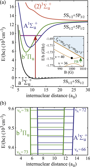
Figure 1. (a) Spectroscopy scheme. Weakly bound Feshbach molecules are irradiated by a laser pulse and excited to molecular levels of the  manifold from where they spontaneously decay to nonobserved states. The potential
  is included because it couples to
  of
of  (see text). Furthermore, the inset shows the level structure in the vicinity of the FR. At a magnetic field of
  G the Feshbach state (indicated by the black circle) is located
  below the
  dissociation threshold at
  G. In (b), the vibrational levels vA and vb within the
  complex that are relevant for our measurements are depicted. All potential curves are taken from [27], while the energies of vA and vb correspond to the calculated values given in [28] (see also tables 1 and 2).
Download figure:
Standard image High-resolution imageThis article is organized as follows. In section 2, we give an overview of the experimental setup and the spectroscopy scheme. Then, section 3 describes the relevant molecular energy states needed for the presentation of our experimental results in section 4. In section 5 we introduce a simple model that fully explains the characteristics of the observed spectra. Our model calculations are discussed in section 6 along with the interpretation of the data and the determination of Δ for the investigated vibrational states of  . Finally, in section 7 we describe the extension of the potential scheme needed for modeling the observations by coupled channel calculations.
2. Experimental setup
We carry out our experiments with a pure sample of about  weakly bound
  Feshbach molecules which have both
  and
and  character. The setup and the molecule preparation scheme are described in detail in [29, 30]. Therefore, they are just briefly presented here. Initially a BEC or ultracold thermal cloud of spin-polarized
  atoms with total angular momentum f = 1,
  is loaded into a rectangular, 3D optical lattice at a wavelength of
  nm, which is formed by a superposition of three linearly polarized standing light waves with polarizations orthogonal to each other. By slowly crossing the magnetic Feshbach resonance (FR) at
  G from high to low fields, pairs of atoms in doubly occupied lattice sites are converted into weakly bound molecules. Afterwards, the magnetic field is set to
  G, where we perform the spectroscopy. In order to get rid of remaining atoms, a combined microwave and light pulse is applied which removes them from the lattice. We end up with a pure ensemble of molecules that resides in the lowest Bloch band of the optical lattice with no more than a single dimer per lattice site. The lattice depth for the molecules with respect to each of the standing light waves of the optical lattice is about
  , where
  represents the recoil energy. Here, m denotes the mass of the molecule and h is Planck's constant. Since at these lattice depths the tunneling rate is very small, intermolecular collisions are strongly suppressed, and we measure lifetimes on the order of 1 s.
Figure 1(a) shows the spectroscopy scheme. The Feshbach molecule ensemble is irradiated by a rectangular light pulse for a duration τ of typically a few ms. At the location of the molecular sample the beam waist is about 1.1 mm. For the observed spectra, we used laser powers of tens or hundreds of  . The light propagates orthogonally to the quantization axis which is defined by the applied magnetic field that points in vertical direction. By using a half-wave plate we can choose the light being polarized either in the horizontal plane or in the vertical axis giving rise to σ transitions (i.e.
  and
and  ) or π transitions. Molecules, that are resonantly excited from the Feshbach state (FS) to a level of the
  complex, are in general lost due to subsequent fast decay to nonobserved states. We measure the remaining fraction
  of Feshbach dimers. For this purpose, we dissociate the molecules by ramping back over the FR and detect the corresponding atom number via absorption imaging.
The spectroscopy is performed at wavelengths between 1042 and  nm (corresponding to about 9360–9600
  ) using a grating-stabilized cw diode laser that has a short-term linewidth of
  kHz. This laser is frequency-stabilized to a Fizeau interferometer wavemeter (High Finesse WS7), with an update rate of about 10 Hz. As the laser frequency drifts between updates, we obtain a frequency stability of
  MHz. The wavemeter is calibrated to an atomic
  reference signal at
  nm in intervals of minutes. It has a specified absolute accuracy of
  MHz, but the accuracy is on the MHz level for difference frequency determinations within several hundred MHz. Furthermore, over a period of several months we checked the frequency readings of the wavemeter for the same molecular transitions and did not find deviations of more than
  MHz. This demonstrates the good reproducibility of the wavemeter readings in connection with the calibration mentioned above.
3. Relevant states
3.1. Feshbach molecules
The  Feshbach molecules in our experiment are weakly bound dimers with both singlet and triplet character, i.e. the selected state is a mixture of
  and
and  [30, 31]. However, only the
  component allows to drive transitions to the
  complex because for an electric dipole transition the
  symmetry has to change and the
  complex has u symmetry. According to coupled channel calculations, at a magnetic field of 999.9 G the singlet component, mainly characterized by
  , I = 2,
  , F = 2, contributes 16% to the Feshbach state (FS) which has the exact quantum numbers
  and parity +. Here, S, L, R, I and F (
 ) denote the quantum numbers of the total electronic spin, the total orbital angular momentum, the rotation of the atom pair, the total nuclear spin, and the total molecular angular momentum, respectively. Furthermore, mI and mF represent the corresponding projections onto the quantization axis. Consequently, the singlet component of the Feshbach molecules has J = 0 (
 ).
).
The inset of figure 1(a) shows the molecular level structure in the vicinity of the FR. Throughout the present work, all excitation energies are given with respect to the  atomic dissociation limit at
  G. Note, its energy is
  below the atomic dissociation limit when hyperfine interaction is ignored. At a magnetic field of
  G the FS is located at
  . Here, the main contribution is determined by the Zeeman shift of the atom pair
  . The molecular binding energy is only about
  with respect to this threshold.
3.2.
 complex

Spin–orbit interaction leads to a mixing of the states  and
and  forming the
  complex. In a simple approach this mixing comes about in two steps. First, due to spin–orbit coupling the state
  splits up into three components,
  . The quantum number Ω denotes the projection of the sum of all electronic angular momenta onto the internuclear axis and equals the projection of the molecular angular momentum J on the same axis. For
  the relative separation of the three terms is about
  , as mainly determined by the atomic spin–orbit splitting of
  in its
  state. At this stage, the
  ,
,  state has two degenerate components,
  and
and  . Second, spin–orbit coupling mixes
  (i.e.,
  symmetry) and
 , whereas the
 component couples to
 (see figure 1(a)). As a consequence of the repulsive interactions
  and
and  of
of  are separated from each other, which is referred to as Λ-type splitting [32]. This effect is crucial for the interpretation of the observations of the present work.
The vibrational levels of the  states relevant to our measurements are illustrated in figure 1(b). The levels with dominant triplet (singlet) character are indicated by vibrational quantum numbers vb (vA). Moreover, tables 1 and 2 list the numerical values for the term energies and the b state admixtures calculated by Drozdova et al [1] and taken from [28]. The calculation is based on a two-potential approach considering
  and
and  (
( ). The mixing is described by the parameter pb, which represents the probability of finding the vibrational level in the electronic state b. Consequently, for the A state the corresponding parameter is given by
  . All other admixtures like
  are negligible in our cases. Our spectroscopy scheme addresses only the A component of a vibrational level of the
  manifold. Moreover, only states with angular momentum J = 1 and negative parity can be observed, because the electronic singlet component of the Feshbach molecule has the quantum number J = 0 and positive total parity.
Table 1.
Comparison of calculated ( ) and measured (
 ) level energies for various vibrational levels vA of the
  state with J = 1. All level energies
  are observed with π-polarized light. The column
  gives the difference of the measured and predicted values. Furthermore, the parameter pb denotes the admixture of the
  potential and δ represents the measured frequency difference between the σ and the π resonance. For the case of
  , 68 and 70 we only performed spectroscopy using π-polarized light and therefore δ was not determined. The values for pb and
  are taken from [28].
| vA | pb |

|

|
 |
δ |
| (%) | ( ) ) |
( ) ) |
( ) ) |
( ) ) |
|
| 66 | 15.60 | 9388.005 | 9387.9967 | 8.3 | −2 |
| 67 | 28.50 | 9423.589 | 9423.5794 | 9.6 | |
| 68 | 23.21 | 9454.571 | 9454.5652 | 5.8 | |
| 69 | 7.66 | 9491.049 | 9491.0451 | 3.9 | −2 |
| 70 | 10.82 | 9525.742 | 9525.7346 | 7.4 | |
| 72 | 39.36 | 9594.454 | 9594.4485 | 5.5 | −22 |
4. Experimental observations
4.1. Spectra of A levels
We first discuss the data for levels with mainly  character. Six different vibrational states (
 –70 and 72) have been investigated. The obtained spectra for
  –70 look very similar. Figure 2(a) shows the recording for
  as an example. Two resonance dips are visible, one being the π transition (
 ), while the other one is the σ transition (
 ). Within the measurement uncertainty of a few
  both resonances are located on top of each other and Zeeman or hyperfine splitting is not observed. We determine the transition frequencies from fits to the data using the function
  , where the amplitude K is a free fitting parameter and L represents a Lorentzian. Typically, the obtained transition linewidths (FWHM) are on the order of 10–20 MHz.

Figure 2. Loss resonances for excitation of molecules from the Feshbach state to vibrational levels  (a) and
  (b) of the
  potential obtained with π-polarized light (black squares) and σ-polarized light (red circles). Shown is the fraction
  of remaining Feshbach dimers dependent on the detuning δ, where
  is at the resonance frequency of the strong π transition. The corresponding offset energies are listed in table 1. Solid lines are fits of the function
  to the data (see section 4.1). For a given vibrational quantum number vA the measurements with π- and σ-polarized light are performed using the same laser intensities and pulse lengths. Colored vertical lines in part (b) indicate the frequency positions of the levels
  resulting from our model calculations (see section 6).
Download figure:
Standard image High-resolution imageIn table 1 the absolute energies of states vA derived from the π resonances are summarized and compared to theoretical predictions. The admixing parameter pb and  are taken from [28]. Since, the calculations were originally given with respect to the potential minimum of
  , for the comparison to our experimental results, we added the electronic term energy
  of
of  [31] and the hyperfine shift of
  , where c is the speed of light. The overall agreement between the theoretical and experimental data is within the uncertainty of the theoretical predictions of
  (corresponding to
  ). Noticeably, the calculated values are systematically higher by several
  compared to our measurements. Besides a possible systematic uncertainty within the theoretical model, these deviations can also arise from the limited accuracy of our wavemeter and the uncertainty of the energy
  .
.
In contrast to the states  and 69, where both, the π and the σ transition occur at the same frequency within the measurement uncertainty,
  shows a significant splitting (see figure 2(b)). This is due to the fact that the admixing of the b state is relatively large (
 , see table 1) and a
 level is located energetically close-by. The level
  significantly exhibits the characteristics of
 , which will be discussed in the following sections.
4.2. Spectra of b levels
Our spectroscopic data on states with mainly triplet character, i.e.,  , are shown in figure 3. For all investigated vibrational quantum numbers
  –76 and 78 we only clearly observe a single resonance dip when using π-polarized light. Contrary to that, the scans related to σ polarization reveal 2 or 3 resonance features of which some might have an unresolved substructure. In each spectrum, the σ transitions are well separated from the π transition. We therefore choose the π resonance as a local reference to which we assign the frequency
  in the figures.
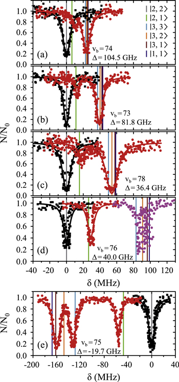
Figure 3. Loss spectra for excitation of molecules from the Feshbach state to vibrational levels  (a),
(a),  (b),
(b),  (c),
(c),  (d), and
  (e) of the
  potential obtained with π-polarized light (black squares) and σ-polarized light (red circles). Here, Δ is the frequency spacing between the 0− and 0+ components of
  (see section 6). All other parameter denotations, the fit function and the meanings of the vertical lines are identical to those of figure 2. The offset energies corresponding to the transitions at
  are given in table 2. For
  and 74 the intensity and pulse length of the σ-polarized light was the same as for π polarization. The spectra of
  (
( ) were measured with different pulse lengths τ, where the ratio was
  (
( ). Concerning
  , data of two scans with σ-polarized light are shown (magenta and red). Whereas the magenta data points were obtained using the same pulse area as for π polarization, it was by a factor of 8 larger when measuring the red data points.
Download figure:
Standard image High-resolution imageAt first sight the spectra for  –76 and 78 might look somewhat irregular. For different vibrational levels vb the number of transitions, their splittings, and their relative intensities vary. In addition, the splittings for a given vb are not equidistant as mentioned earlier for high J. However, closer inspection reveals that all these spectra are characterized by a similar pattern. To show this, we arrange the spectra in the order
  , 73, 78 and 76 (figures 3(a)–(d)) corresponding to their respective splitting magnitude. In each spectrum the σ lines are located at
  . There is always one weak resonance next to the π transition and one strong resonance feature at larger δ. For
  , where the total splitting is very large, the resonance dip at
  MHz seems to split up into two or more lines. Due to the limited resolution of about
  MHz in our experiment we can not clearly resolve the individual resonance lines, but the observed fluctuations in the number of molecules are a clear indication of an internal structure of this resonance dip.
In contrast, the spectrum of  (figure 3(e)) is inverted compared to the spectra discussed before and exhibits three σ resonances, all of them at
  . As it is spread over an even larger frequency range of about
  MHz, the resonance dips at
  and
and  are clearly separated from each other. The offset energies for the observed lines at
  are listed in table 2 and are compared to the theoretical predictions of [28]. Again, the agreement is within the theoretical uncertainty. However, we note that the measured π transitions contain shifts due to hyperfine and Zeeman interaction. These shifts of up to
  MHz (see section 6) would need to be subtracted for a proper comparison of the data with the calculations of [1].
Table 2.
Comparison of calculated ( ) and measured (
 ) level energies for various vibrational levels vb of the
 state with J = 1, analogous to table 1. The parameter Δ is the splitting of the
  components as determined by fitting our theoretical model to the measured spectra (see section 6).
| vb | pb |

|

|
|
Δ |
| (%) | ( ) ) |
( ) ) |
( ) ) |
( ) ) |
|
| 73 | 82.70 | 9368.758 | 9368.7480 | 10.0 |

|
| 74 | 69.59 | 9412.519 | 9412.5122 | 6.8 |

|
| 75 | 73.80 | 9460.874 | 9460.8718 | 2.2 |

|
| 76 | 88.37 | 9503.516 | 9503.5040 | 12.0 |

|
| 78 | 58.25 | 9591.479 | 9591.4721 | 6.9 |

|
5. Simple model of the molecule
In principle, hyperfine and Zeeman interaction within the  state of diatomic molecules has been theoretically investigated in depth (see, e.g., the 4th-order perturbation approach of [33]). However, properly applying such theoretical (and often complex) approaches to interpret measured spectra can still be a challenge because of the large number of parameters for representing the different orders. Therefore, we have developed a simple model which neglects some fundamental properties of a molecule. Nevertheless, it should be adequate to explain semi-quantitatively the Zeeman and hyperfine structure observed in our spectra.
In our model, the  molecule is treated as a rigid rotor with fixed internuclear separation. Consequently, there is no vibrational degree of freedom. However, the positions of the nuclei can be interchanged. This is necessary in order to construct fully antisymmetric wave functions for the system of the two nuclei and the two valence electrons owing to the particles' fermionic character. Essentially, we consider the molecule as if it was composed of two unperturbed neutral atoms, of which, however, the angular momenta
  and
and  are strongly coupled to the rigid rotator axis. In each of the atoms the orbital angular momentum Li of the local electron i is a good quantum number. Thus, molecules belonging to the atom pair
  have both a p-orbital with
  and an s-orbital with
  , and the total orbital angular momentum is L = 1 (
 ). Therefore, the two valence electrons can never be found in the same orbital. Coupling the electrons to the rotator axis (which corresponds to the internuclear axis) forms the electronic states
  of the molecule. For simplicity, in the following discussion we restrict the model to those electronic states that are most relevant to describe our observations, i.e., states with u-symmetry and
  . These are
  (
( as well as
  ),
),  and
and  (see section 3.2).
The molecule is described by the Hamiltonian

which, in addition to a diagonal energy matrix, contains spin–orbit coupling, nuclear rotation, hyperfine and Zeeman interaction. The diagonal energy matrix

sets the initial values for the energies  of the electronic levels
  before the remaining terms of the Hamiltonian are turned on. Here,
  denotes the projector onto the respective state. In order to describe the hyperfine and Zeeman structure for a given vibrational level v' (with symmetry
  ), the influence of all surrounding vibronic levels for each symmetry is mimicked by a single, effective energy value
  . As an example, let us assume that we want to describe the hyperfine and Zeeman structure of the vibrational level
  of the b state. As can be seen in figure 1(b),
  is surrounded by several vA levels in its proximity, with
  , 68 and 69 being the closest ones. All these vA levels are replaced by a single effective vibrational level with energy
  in our model.
The second term of equation (1) is the spin–orbit interaction

which couples spin  and orbital angular momentum
  of electron i. Here,
  denotes the spin–orbit parameter being the corresponding atomic value divided by two because we have only
  probability for each electron to be in the p-orbital. From the atomic fine structure in
  (see, e.g. [34]) one obtains
 ![${C}_{\mathrm{SO}}=\left[E({5}^{2}{P}_{3/2})-E({5}^{2}{P}_{1/2})\right]/(3{{\rm{\hslash }}}^{2})=2374\;\mathrm{GHz}\times h/{{\rm{\hslash }}}^{2}$](https://content.cld.iop.org/journals/1367-2630/17/8/083032/revision1/njp517383ieqn266.gif) . We use this value of
. We use this value of  for the spin–orbit interaction between
  and
and 
 . These states are separated by about
  (see figure 1(a)). The corresponding level repulsion shifts the
 component to lower energies by several tens of
  compared to the situation, when spin–orbit interaction is ignored. For the spin–orbit coupling between
  and
and 
 , we additionally take into account the overlap integral of the relevant vibrational wave functions, which is typically ∼0.1 for states of the considered frequency range (9360–9600
  ). The spin–orbit interaction is responsible for the frequency splitting Δ between the
  and
and  components of
  and the mixing of the A and b state which is expressed in terms of the admixing parameter pb. It turns out that Δ and pb are the two quantities, which essentially determine the hyperfine and Zeeman structure of a vibrational state. By fine tuning Δ and pb in our model we can describe the observed spectra. For practical purposes, we vary neither
  nor the value of the overlap integral (
 ), instead we use the term energies of the relevant uncoupled states in
  . Concretely, we adjust pb by setting the separation between
  and
and  , while the size of Δ is adjusted by shifting the term energy of the
  level relative to the
  level.
The third term of equation (1),

describes the rotation of the atom pair. According to the calculations of Drozdova et al [28], the rotational constant Bv is about  for the
  states with dominant b character and vibrational quantum numbers
  70–80 of
  . The quantum number of angular momentum
  appearing in the atom pair basis determines the total parity of the molecular state according to
  . But R is not a good quantum number for the molecular eigenstates since
  does not commute with HDiag.
Next, we consider the hyperfine interaction HHF. As mentioned in [4], the Fermi contact term is in general sufficient to characterize the hyperfine interaction of alkali-metal dimers. We use

with  and
and  . According to [4, 35, 36], the Fermi contact parameter bF for an atom pair (
 ) is
) is  , where
  denotes the atomic hyperfine parameter for the
  level of
  [37]. We note that this ansatz is formally identical to the atomic hyperfine interaction of a ground state electron (i.e. s-orbital) with its local nuclear spin Ii. The factor
  normalizes the interaction because at any instant in time only one of the two electrons (i.e. the s-electron) interacts with only one of the two nuclei. We fix the Fermi contact parameter to be
  but note that deviations of up to
  from this approximation have been observed, e.g. for
  [36]. We do not use bF as a free fit parameter in our model because it is strongly correlated with the unknown frequency splitting Δ (see section 6). Thus, any uncertainty in bF directly translates into an uncertainty of Δ. Furthermore, by using the ansatz of equation (5) we neglect the nondiagonal part of the hyperfine interaction with respect to S and I and thus there is no mixing of
  symmetry. However, this approximation should be valid as the energy spacing between possibly coupled
  states is significantly larger than the
  spacing considered in this work.
The last term of equation (1) characterizes the Zeeman interaction in a homogeneous magnetic field of strength B in z direction

with  being Bohr's magneton. Here, we consider the Zeeman interaction due to the orbital angular momenta of the electrons, the electronic spins as well as the nuclear spins, where
  ,
,  and
and  for
for  [37] are the corresponding g-factors.
The matrix elements are calculated in an uncoupled atom pair basis, being a properly antisymmetrized product of eigenstates of all needed angular momenta and their projection on the space-fixed axis z, and the nuclear positions at both ends of the rotator axis. Table 3 gives an overview of the range of quantum numbers for the  states of
  , which are needed to setup the matrix. The total molecular angular momentum J (
 , i.e., without nuclear spins) is a fairly good quantum number, because the hyperfine and Zeeman interaction is small compared to the other interactions.
Table 3.
Overview of the range of quantum numbers for states  and
and  of
of  with low angular momentum J. The +/-columns provide the total parity whereas I represents the total nuclear spin and R is the atom pair rotation. Note that the quantum numbers I and parity alternate with J. This behavior is also found for the even and odd values of R. Furthermore, the molecular rotation increases with J.

|

|
|||||
| J | I |

|
R | I |

|
R |
| 0 | 1, 3 | + | 1 | 0, 2 | − | 0, 2 |
| 1 | 0, 2 | − | 0, 2 | 1, 3 | + | 1, 3 |
| 2 | 1, 3 | + | 1, 3 | 0, 2 | − | 0, 2, 4 |
| 3 | 0, 2 | − | 2, 4 | 1, 3 | + | 1, 3, 5 |
| 4 | 1, 3 | + | 3, 5 | 0, 2 | − | 2, 4, 6 |

|

|

|

|

|

|
⋮ |
6. Model calculations and interpretation of measured data
In the following we use the model introduced in the previous section to calculate the Zeeman and hyperfine structure for an  bound state as a function of the frequency splitting
 ![$\Delta =[E({0}^{-},J=0)-E({0}^{+},J=1)]/h$](https://content.cld.iop.org/journals/1367-2630/17/8/083032/revision1/njp517383ieqn333.gif) of the
of the  components of
  3
, the degree of mixture pb between the A and b states, as well as the magnetic field B. We define Δ to be the splitting between
3
, the degree of mixture pb between the A and b states, as well as the magnetic field B. We define Δ to be the splitting between  after diagonalization of the Hamiltonian H of equation (1). In order to keep the discussion simple, we restrict ourselves to the range of quantum numbers and parameters directly related to our experiments. As explained in section 3.2, starting from Feshbach molecules we can only optically excite
  bound levels through the
 component with angular momentum J = 1 and negative parity. Furthermore, we want to point out that the eigenstates of the Hamiltonian of equation (1) are eigenstates of the total nuclear spin I. Thus, we can restrict ourselves to bound states with I = 2, being equal to the value of the singlet component of the FS applying the electric dipole selection rule
  .
.
The diagonal Zeeman and hyperfine interactions of the states  are negligible compared to our measurement uncertainty. However, both the Zeeman interaction
  and the hyperfine interaction
  couple
  and
and  within
  . In particular, (J = 1, I = 2) of
  couples to (J = 0, I = 2) and (J = 2, I = 2) of
  (see table 3). This leads to mixing, i.e., to the creation of eigenstates with a net electronic magnetic moment and thus to Zeeman and hyperfine splittings. Interestingly, hyperfine and Zeeman interaction amplify the line splittings in a cooperative way because they have matrix elements for the coupling between
  and
and  similar in magnitude and equal in sign. Hence, if Zeeman and hyperfine interaction are of the same strength their combined effect increases the line spacings not only by a factor of 2 but by a factor of 4. Our experiments are indeed close to this regime for the selected magnetic field of about
  G.
G.
The Zeeman and hyperfine splitting crucially depends on the frequency spacing Δ between the levels  and
and  of
of  . Using standard perturbation theory, the splitting is estimated to be proportional to
  . We recall that the spin–orbit couplings to
  and
and  generate the spacing Δ between the levels
  and
and  of
of  in the restricted Hilbert space.
Figure 4 depicts results of our model calculations for a vibrational level of  with
with  triplet (b) and
  singlet (A) character. The frequency positions of levels
  are shown as a function of Δ for two magnetic fields,
  and
and  G. Although the total angular momentum F' is generally not a good quantum number anymore at higher magnetic fields, we refer to the molecular levels by the correlated value of F' at
  G. In figure 4 only those six states
  are plotted that, according to the electric dipole transition selection rules, are accessible by our spectroscopy experiment. As the Feshbach molecule has F = 2,
  , levels with the quantum numbers
  (
( ) can be observed via π (σ) transitions. We choose the state
  as energy reference (i.e.,
  ), because it corresponds to the strong π resonance in figures 2 and 3. This allows for convenient comparison of our calculations to the measured spectra. Note, at
  G, no mF splitting can occur and therefore only three different curves are discernible in figure 4(a).
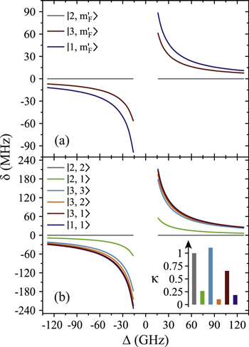
Figure 4. Hyperfine level structure for a vibrational state vb with  for two magnetic fields,
  G (a) and
  G (b). Shown are the frequency positions δ of the levels
  relative to the state
  , as a function of Δ. The inset in (b) gives the relative strengths κ for the optical dipole transitions from the Feshbach state towards the levels
  of vb at
  G. For
  we set
  . For convenience, we have plotted the same data in figure A1 in terms of
  . This makes it easier to read off the line splittings for small
  .
.
Download figure:
Standard image High-resolution imageIn our calculations, Δ is set by adjusting the initial energy spacing between the  and
and  components of the b state in
  (see equation (2)). To a good approximation, within the frequency ranges considered in figure 4 (i.e.
  = 16–129 GHz) the level splittings increase inversely with Δ, just as expected from perturbation theory. This can directly be seen in figure A1
of the appendix. For
= 16–129 GHz) the level splittings increase inversely with Δ, just as expected from perturbation theory. This can directly be seen in figure A1
of the appendix. For  G and a small
  of
of  GHz, the overall spreading of the levels reaches more than
  MHz, whereas for a large
  GHz it is on the order of a few tens of
  or less. Furthermore, the ordering of the energy levels is inverted, when the sign of Δ changes. We point out that some level spacings are smaller than the expected linewidths and therefore can not be resolved in the experiment. The widths of the levels are mainly determined by those of the
  state (
 MHz) and the admixing parameter pA, because the width of the pure
  state is orders of magnitude smaller compared to the one of
  . The basic structure of the calculated levels (see figure 4) and the level widths let us expect to resolve three resonance features which agrees well with our observations shown in figure 3.
We now want to assign the experimentally observed resonances to distinct transitions. Besides considering the line positions we also take into account the strength of the lines. For this purpose, we calculate the dipole matrix elements  from the initial Feshbach state
  to the final levels
  of the mixed
  state. As already mentioned, we only have to consider the singlet component of both levels. The inset in figure 4(b) shows the relative transition strengths
  at
at  G. We can roughly group the six transitions into three strong ones (by σ light towards final states
  and
and  , by π light towards
  ) and three weak transitions (σ: towards
  and
and  and π: towards
  ). Our observed spectra always exhibit only one strong line for π-polarized light (see figure 3). It is therefore assigned to
  and used as reference level. The calculations predict a second resonance for π polarization which should be about one order of magnitude weaker. However, we did not unambiguously observe this line since its signal is easily drowned by the overlaying strong σ lines if the achieved light polarization is not sufficiently pure.
In the following, the σ transitions are discussed in detail using the results shown in figure 4(b). Although the transition towards  is weak, we should be able to clearly observe it, since the level
  is well separated from all other levels. The three remaining transitions (towards
  ,
,  and
and  ), however, are quite close to each other. Especially for larger values of
  (
( GHz) these levels can not be resolved and only a single resonance should be visible. Among the three transitions, the one towards
  is most dominant. For low values of
  (
( GHz) the strong
  line splits clearly from those corresponding to
  and
and  which both barely separate. This explains why our observed spectra for σ-polarized light in figure 3 exhibit at most three resonance features. At this stage we have shown that the experimental data can be qualitatively explained by our theoretical model and that we already can assign quantum numbers to the measured resonance lines.
Now, we want to carry out a more quantitative comparison of the measured line splittings in figure 3 with the model predictions. For this, we study the dependence of the energy level structure on the admixing parameter pb, i.e. the percentage of the  potential in the vibrational state vb. In the simulations, we set pb by adjusting the term energy of the bare
  state in equation (2). Results for
  GHz are shown in figure 5. To good approximation, within the investigated range from
  to
to  the level frequencies depend linearly on pb. This makes sense as the discussed hyperfine and Zeeman interaction only appears within the
  (
( ) state.
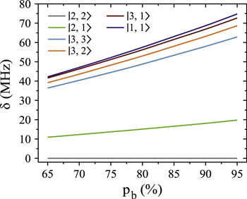
Figure 5. Dependence of the hyperfine and Zeeman structure on the admixing parameter pb for a fixed value of  GHz and a magnetic field of
  G. The frequency δ is given relative to the
  level.
Download figure:
Standard image High-resolution imageIn order to carry out the quantitative comparison for each spectrum vb, we individually fix the splitting of the bare 
 and
and 
 levels such that the admixing parameter pb equals to its literature value [1, 28], as listed in table 2. Afterwards, we fit our model to the measured spectrum by adjusting a single parameter, the effective term energy of
 in HDiag and thus the splitting Δ between the
  and
and  components of the b state. All other parameters of the model are kept at the values given in section 5. For the fit, we ignore the states
  and
and  since they can not be experimentally resolved (see inset of figure 4(b)). The resulting spectral positions of the hyperfine levels are shown in figure 3 as vertical lines together with the measured spectra. The agreement is quite satisfactory as the experimental and calculated line positions do not differ by more than a few MHz. Our fit results for Δ, i.e. the splitting of the
  states after diagonalizing the Hamiltonian H of equation (1), are listed in figure 3 as well as in table 2. We obtain values ranging from
  to
to  GHz. The error boundaries for Δ in table 2 are estimated by simulations shifting the resonance frequency δ of the strong
  line by
  MHz relative to the reference
  . Such an approach is reasonable as the frequency stability in our measurements is
  (2–5) MHz. In addition to these error boundaries there exists a further uncertainty in Δ, since the precise value of the hyperfine interaction parameter bF is unknown. As already discussed in section 5, we expect that our adopted value for bF possibly deviates by up to
  from its real value. According to the simple estimation for the hyperfine and Zeeman splittings (
 ), such a change in
  leads to a similar change of
  from the fit. In our data analysis, we have verified that the fits to the measured spectra remain of similar quality when we vary bF by a few tens of
  .
.
Next, we investigate the Zeeman and hyperfine structure as a function of the magnetic field. Figures 6(a) and (b) depict the model calculations for the vibrational levels  and 73, respectively, using the values of pb and Δ given in table 2. For both plots the admixing parameters are similar (
 ), while the respective frequency spacings Δ have different signs and magnitude. We show all the levels accessible in our spectroscopy together with the experimentally derived levels at
  G. Here, the frequency reference is represented by the level
  at this magnetic field. We present in figure 6(c) the full hyperfine and Zeeman structure of a single state vb for
  GHz,
GHz,  . This graph reveals particularly well the transition from the linear Zeeman effect to a quadratic behavior above a few hundreds of gauss and the enhancement of the splitting by the cooperative effect between Zeeman and hyperfine interaction.
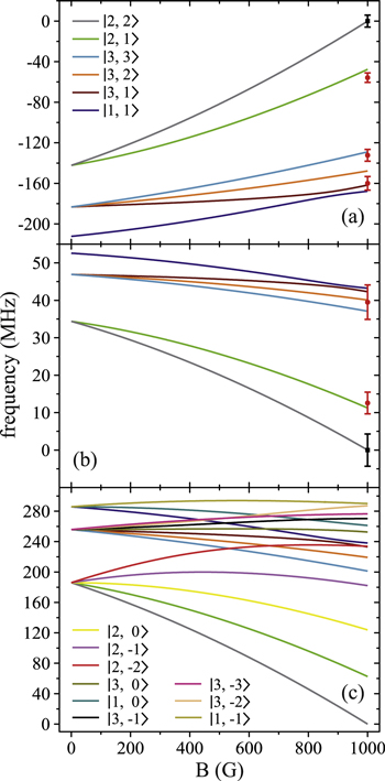
Figure 6. Zeeman structure of the hyperfine levels  as a function of the magnetic field B. The frequency is referenced to the position of level
  at
at  G. (a) Simulations for
  GHz,
GHz,  , (b) for
  GHz,
GHz,  and (c) for
  GHz,
GHz,  . The black square (red dot) plot symbols indicate the experimentally observed resonances obtained with π-polarized (σ-polarized) light corresponding to
  (a) and 73 (b). The error bars represent the measured transition linewidths (FWHM) determined from our fits to the data (see figures 3(b) and (e)). In (c), all hyperfine energy levels of the vibrational state vb (J = 1, I = 2) are plotted, where the color code is extended for the additional levels compared to (a) and (b).
Download figure:
Standard image High-resolution imageFinally, we want to give a quantitative interpretation of the spectrum corresponding to the vibrational level  of
of  (see figure 2(b)), which has a large b state admixture (
 ) due to the strong coupling of
  to
to  as these states are fairly close to each other. The separation is only
  GHz according to tables 1 and 2. For
  , our model determines a spacing of
  GHz between its
  and
and  components. Consequently, the
 state is only separated by
  from the
 state. From this, we can predict the hyperfine structure for
  with our model. The results are shown in figure 2(b). As can be seen, the calculated and measured resonances agree well, which nicely confirms the consistency of our model.
7. Splitting between and components in a potential scheme


In the previous section, we have determined the effective splitting ![$\Delta =[E({0}^{-},J=0)-E({0}^{+},J=1)]/h$](https://content.cld.iop.org/journals/1367-2630/17/8/083032/revision1/njp517383ieqn501.gif) for the state
for the state  using our simple model without vibrational degree of freedom. Here, we compare the obtained results to those of coupled channel calculations with a potential scheme, i.e. including the full dynamics of the relative motion within the atom pair. As a first step we follow [1] and therefore restrict the calculations to the
  system, such that the spin–orbit interaction and the molecular rotation only couple the A and b states. Thus, the influence of the spin–orbit coupling of
 to
to 
 is not yet considered. The term values for the
  complex are listed in table 4. For the calculations we take the model potentials and spin–orbit functions reported in [1]. Columns 3 and 4 show the term values for
  , J = 1 and
  , J = 0 in the absence of spin–orbit coupling, respectively. At this stage, the
  and
and  components of the
  state are only split due to rotation. Column 5 lists the term energies for
  , J = 1 if the spin–orbit coupling is included. These are the same values as given in tables 1 and 2. Column 6 provides the energy difference of each
  state in column 4 relative to the closest
  state in column 3. This quantity, which we call
  , is the prediction for the
  splitting within the
  system. Noticeably,
  varies strongly for different vibrational levels, which results from the fact, that the uncoupled vibrational ladders vA and vb of
  and
and  are interwoven with different spacings. Thus, their repulsion due to the interaction of different vibrational levels is fairly irregular. Column 7, labeled
  , recalls the findings for Δ inferred from our measurements. There is disagreement between the measurements and the results of the restricted coupled channel model. All values
  are significantly larger (more positive) than
  . However, it is striking that the differences between
  and
and  , are all close to
  GHz. The actual values are given in column 8, where the uncertainties are taken from
  (see, e.g. table 2). Indeed, all differences (except for
  ) are equal within the given uncertainties. Could the spin–orbit coupling to state
  be responsible for this discrepancy of
  GHz? No, it can not. Indeed, the
  state is far up in energy (see figure 1(a)) and therefore all vibrational levels of
 experience an almost constant shift, but it has the wrong sign to explain the observations. If ab initio calculations for the
  potential energy curve and the corresponding spin–orbit interaction are applied, we obtain quantitatively that the
  component of the
  state is shifted by about
  to lower energies. This increases the deviation of already
  GHz to about
  GHz, much beyond experimental uncertainties.
Table 4.
Energy levels of the component  of
of  and of
  without (w/o SO) and with (w SO) spin–orbit coupling. Column 3 shows the calculated energies for
  of the A and b states for J = 1, whereas column 4 contains only energy levels for
  and J = 0. In column 5 the corresponding values for
  and J = 1 are provided, obtained with the spin–orbit interaction between states A and b. Column 6 reports the splittings
 ![$[E({0}^{-})-E({0}^{+})]/h$](https://content.cld.iop.org/journals/1367-2630/17/8/083032/revision1/njp517383ieqn548.gif) calculated for the restricted system
calculated for the restricted system  and denoted by
  , while column 7 lists the results derived from our experiments. (For details see text.)
| State | vA, vb |
 , J = 1 , J = 1 |
 , J = 0 , J = 0 |
 , J = 1 , J = 1 |

|

|

|
| (w/o SO) | (w/o SO) | (w SO) | |||||
( ) ) |
( ) ) |
( ) ) |
(GHz) | (GHz) | (GHz) | ||

|
65 | 9352.911 | 9352.078 | 534.3 | |||

|
73 | 9369.939 | 9369.901 | 9368.758 | 34.3 | 81.8 |

|

|
66 | 9388.026 | 9388.005 | −542.7 | |||

|
74 | 9414.679 | 9414.641 | 9412.519 | 63.6 | 104.5 |

|

|
67 | 9423.000 | 9423.589 | −268.3 | |||

|
68 | 9457.834 | 9454.571 | 137.9 | |||

|
75 | 9459.210 | 9459.172 | 9460.874 | −51.0 | −19.7 |

|

|
69 | 9492.527 | 9491.049 | 373.0 | |||

|
76 | 9503.529 | 9503.492 | 9503.516 | −0.7 | 40.0 |

|

|
70 | 9527.078 | 9525.742 | 655.2 | |||

|
77 | 9547.635 | 9547.598 | 9547.629 | −0.9 | ||

|
71 | 9561.487 | 9560.041 | −373.0 | |||

|
78 | 9591.525 | 9591.488 | 9591.479 | 0.3 | 36.4 |

|

|
72 | 9595.754 | 9594.454 | −88.9 | −52.8 |

|
|

|
73 | 9629.979 | 9627.657 | 224.9 |
Because the energetic order of the  components is accurately determined from former spectroscopic work [1], our observation directs clearly to the spin–orbit energy of the
  component of state
  . Interestingly, the spin–orbit functions of
  presented in figure 6(a) of [1] are different for
  and
and  by about
  as derived from the reported amplitude
  of the spin–orbit function in table 5 of [1]. This difference indicates that
  is no longer a pure spin–orbit multiplet of a Π state. If we consider that a similar deviation of the multiplet structure also exists for
  , then a decrease of about
  compared to the spin–orbit function for
  in [1] would be sufficient to model the
  as given in table 4. We believe that this is a plausible explanation of our observation.
Finally, in view of the calculated splittings of  and
and  we want to recall the measurements for the vibrational levels
  and 69 of
  (see figure 2(a) and table 1). The absolute values
  , even when corrected by the above determined shift of
  GHz, are very large. Therefore, according to the discussion in section 6, we do not expect significant hyperfine and Zeeman splittings. Indeed, no hyperfine structure was observed in our spectra for
  and 69.
8. Conclusion
We have investigated the combined hyperfine and Zeeman structure in the spin–orbit coupled  complex of
  dimers. We performed spectroscopy of ultracold Feshbach molecules at a magnetic field of
  G and recorded the spectra for several excited vibrational levels with either dominant
  character (
 and 72) or dominant
  character (
 73–76 and 78). We observe large line splittings of up to
  MHz and find that the Zeeman and hyperfine structure of the
  state of
  varies strongly for different vibrational levels. Using a simple model, where the molecule is treated as a rigid rotor of two neutral atoms, we can explain the level structures as resulting from nondiagonal hyperfine and Zeeman interactions between the
  and
and  components of
  . The hyperfine and Zeeman interactions act in a cooperative way, which enhances the level splittings. Furthermore, the level splittings depend linearly on the admixture pb for the components
  of the complex
  and
and  , and scale inversely with the frequency spacing Δ between
  and
and  . From fits of our model to the data, we find that Δ strongly varies in the range of
  to
to  GHz within the interval of studied vb and vA. Our observed values for Δ systematically deviate by about
  GHz from predictions of close-coupled channel calculations of the electronic structure correlated to the atom pair asymptote
  using empirical potentials for
  and
and  and ab initio results for
  . We can eliminate this deviation by introducing a spin–orbit–coupling function that is different by
  for
for  and
and  .
.
The fact, that we can extract the frequency spacing Δ from our measurements of the hyperfine and Zeeman structure is a significant result of this work. In ordinary spectroscopy, starting from a ground state molecule only the state  can be addressed, owing to selection rules. Therefore, very little data on the Λ-type doubling of
  is available, so far. Recently, all multiplet components of the
  state were observed in the photoassociation of ultracold
  atoms [38]. The colliding 2S +2S atom pair contains a superposition of states with both symmetries
  (
( and 1) from which
  (
( ) can be reached by electric dipole transitions. To our knowledge, our method represents the first work to experimentally access Δ by investigating only one of the
  components of
  .
.
In the simple model only the hyperfine contribution from the s electron was considered. Thus it is unknown, how much the missing contribution by the p electron and the electric quadrupole interaction might influence the determination of the energy splitting between  and
and  . In this respect and according to the evaluated multiplet structure here, it would be interesting to compare the results of the simple model to full close-coupled channel calculations based on accurate Born–Oppenheimer potential curves including hyperfine and Zeeman interaction with its non-diagonal contributions between the multiplet components. But for this task more experimental data is needed in order to determine the vibrational dependence over a large interval, which allows for deriving r-dependent functional forms of the spin–orbit interaction and probably also of the hyperfine interaction. The latter one was clearly needed in an earlier study on the triplet ground state
  of
of  [31]. We want to emphasize that the strength of the present approach is, that the modeling of all observations on hyperfine and Zeeman splittings are concentrated in an effective single parameter, an average value of the spin–orbit function for
  . The hyperfine parameter and the g-factors are kept constant at their atomic values. This will be altered if a wide range of vibrational levels is studied.
In general, the gained information is valuable for a detailed, fundamental understanding of molecular hyperfine and Zeeman level structures. Despite the already existing long tradition (see, e.g., the early paper by Freed [33]) there is still great interest in this field of research as documented by recent experimental studies, for instance with respect to  [30, 39, 40]. Our results can be exploited for an optimized preparation of ultracold deeply bound ground state molecules either via photoassociation [41] or a stimulated Raman adiabatic transfer starting from Feshbach molecules.
Acknowledgments
The authors would like to thank Anastasia Drozdova and Paul S Julienne for valuable information and fruitful discussions. This work is funded by the German Research Foundation (DFG). ET gratefully acknowledges support from the Minister of Science and Culture of Lower Saxony, Germany, by providing a Niedersachsenprofessur.
Appendix
In figure A1 we show the hyperfine level structure for the parameters of figure 4 but as a function of  . Figure A1 clearly reveals the inverse dependence of the level splittings on Δ in the investigated range of
  16–129 GHz. This representation is more convenient for reading off the splitting for small values of Δ. Furthermore, it becomes obvious that the Zeeman effect enhances the splittings since in (b) the frequency separation of the group of levels characterized by F = 1 and 3 relative to the group corresponding to F = 2 is significantly larger than in (a).
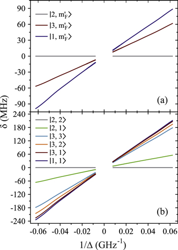
Figure A1. Hyperfine level structure for a vibrational state vb with  for two magnetic fields,
  G (a) and
  G (b). Shown are the frequency positions δ of the levels
  relative to the state
  , as a function of
  .
.
Download figure:
Standard image High-resolution imageFootnotes
- 3
The different J values are required for obtaining the same parity for the mixed states. In addition to J = 0, also the level J = 2 of
will couple to J = 1 of . The rotational energy splitting between J = 0 and 2 of is determined by equation (4).


