


Abstract
We simulate randomly crosslinked networks of biopolymers, characterizing linear and nonlinear elasticity under different loading conditions (uniaxial extension, simple shear, and pure shear). Under uniaxial extension, and upon entering the nonlinear regime, the network switches from a dilatant to contractile response. Analogously, under isochoric conditions (pure shear), the normal stresses change their sign. Both effects are readily explained with a generic weakly nonlinear elasticity theory. The elastic moduli display an intermediate super-stiffening regime, where moduli increase much stronger with applied stress σ than predicted by the force-extension relation of a single wormlike-chain ( ). We interpret this super-stiffening regime in terms of the reorientation of filaments with the maximum tensile direction of the deformation field. A simple model for the reorientation response gives an exponential stiffening,
  , in qualitative agreement with our data. The heterogeneous, anisotropic structure of the network is reflected in correspondingly heterogeneous and anisotropic elastic properties. We provide a coarse-graining scheme to quantify the local anisotropy, the fluctuations of the elastic moduli, and the local stresses as a function of coarse-graining length. Heterogeneities of the elastic moduli are strongly correlated with the local density and increase with applied strain.
Export citation and abstract BibTeX RIS

Content from this work may be used under the terms of the Creative Commons Attribution 3.0 licence. Any further distribution of this work must maintain attribution to the author(s) and the title of the work, journal citation and DOI.
1. Introduction
In this paper we study the elasticity of networks of semiflexible polymers in response to an applied macroscopic strain [1, 2]. In the form of the cytoskeleton or the extracellular matrix, these networks form important building blocks of many biological materials. Their nonlinear and heterogeneous elasticity plays a crucial role in many cell functions.
On long-time scales nonlinear response may be induced via network remodelling [3, 4]. Here, we are interested in time-scales that are short enough, so that crosslinks can be assumed to be permanent, yet long enough for thermal processes to relax. Nonlinear response is then a consequence of the complex elasticity of biological polymer networks as compared to synthetic polymer gels made from flexible polymers [5]. Different mechanisms have been proposed that mediate the strong increase of elastic modulus G with increasing strain γ or stress σ: first, the stretching response of a single semiflexible polymer, as described by the wormlike chain (WLC) model, is strongly nonlinear, and is expected to yield a nonlinear elastic modulus  [6, 7]. Alternatively, it has been argued that a crossover from a soft bending-dominated response to a stiffer stretching dominated response results in an increase of the modulus [8, 9]. Bending in itself is not commonly thought to give rise to strong nonlinear response (see [10] for an exception). Here, we evidence such a regime of nonlinear bending dominated response, that we argue to have its origin in the re-orientation of filaments with the tensile direction of the deformation field. Only when filaments are fully aligned, the WLC nonlinearity kicks in and leads to an asymptotic exponent of
  .
.
Next to nonlinear elasticity, amorphous solids are known to display heterogeneous elasticity. Under an applied strain elements deform in a nonaffine way, as has been shown for glasses [11, 12], biopolymer networks [13, 14], emulsions and granular matter [15, 16]. Furthermore, it has been known for some time [17] that an amorphous structure can support nonvanishing local stresses, even if the sample is stress-free on a macroscopic scale. Given local strains and stresses, the concept of local elastic moduli arises naturally, characterizing soft and hard regions in a disordered environment. In [18], the elastic moduli of a polymeric glass were shown to be strongly heterogeneous on a length-scale on the order of ten monomers. Furthermore, regions with negative local moduli were identified, stabilized by surrounding regions of positive moduli. In simulations of model central-force networks [19], the local elastic constants have been measured and identified as the driving-force for nonaffine displacements. In [20], the fluctuations of the local stress and of the local elastic constants were computed for a simple model of vulcanized polymers. It was shown that correlations of the elastic constants are short-ranged, whereas correlations of the local stress either with itself or one of the elastic constants show power-law decay. A large-scale simulation of a 2D Lennard–Jones glass [12] revealed that the macroscopic shear strain is concentrated in regions of low shear modulus. It also connected these regions to dynamical heterogeneities and plastic events.
From the point of view of elastic heterogeneity, polymer networks are very special and interesting. First, the structure of filamentous networks is, in general, hierarchical and has to be described by several length-scales [21]: next to the monomer size and average mesh-size of the network there is a mesoscopic length-scale that follows from the rod-like appearance of the filaments over scales that are much longer than the mesh-size. Such a length-scale is immediately apparent, for example, in fluorescence-microscopy micrographs of fascin-crosslinked actin-bundle networks [22]. This structural feature sets semiflexible-polymer networks apart from polymer gels made from flexible polymers, or from foam-like architectures where there is only one structural length-scale [23].
Second, stiff polymers are highly anisotropic elastic objects [24], as one can infer already from their extended, rod-like shape. The anisotropy is characterized by the ratio of persistence length  to the typical strand length
  in between two crosslinks. This ratio specifies the relative resistance of the polymer to longitudinal (stretching) forces as compared to transverse (bending) forces. Due to this anisotropy on the network level, it is not immediately clear under what conditions one or the other mode dominates [8, 25, 26].
Third, owing to the large aspect-ratios of the filaments (diameter  , length
  ), networks are rather dilute. The microstructure is therefore heterogeneous, with a broad distribution of mesh-sizes [27]. This, in particular, has to be compared to the homogeneous liquid-like microstructure of amorphous solids.
It is this complex interplay between the network microstructure and the mechanics of individual polymers that generates complex elastic properties [28]. In particular we expect, and indeed find, strongly fluctuating elastic constants. These heterogeneities are expected to be relevant for microrheology experiments, provided the distances over which the elastic response is probed in experiment is comparable to the length-scale characterizing the decay of heterogeneities. Furthermore, plastic events and rupture in the extreme case are likely to be triggered by high strains in soft regions. Hence, knowing the distribution of these regions can serve as a first step to predicting these events.
The paper is organized as follows. In section 2 we introduce the network model which is simulated. In section 3 we discuss global elasticity with emphasis on the nonlinear modulus and the normal stresses. The onset of nonlinear behavior is well accounted for by generic nonlinear elasticity theory. The observed strong shear-stiffening for intermediate stress is explained with a simple model for the reorientation of filaments or strands, giving rise to an exponential increase of modulus with applied stress. In section 4, we explain our coarse-graining procedure and compute the distribution of local stresses, demonstrating the existence of local prestress. We compute the distribution of local elastic constants and study these fluctuations' dependence on the applied strain and degree of crosslinking. A brief conclusion and outlook is given in section 5.
2. Computer-generated crosslinked polymer networks
Our aim is to model as large a crosslinked semiflexible polymer-network as possible. To this end, the polymers' bending degrees of freedom between crosslinks are integrated-out. The remaining degrees of freedom are the crosslink coordinates, which interact with each other via an effective potential; the latter captures the 'lost' degrees of freedom of the polymers. With these assumptions the model is limited to sufficiently low-frequency deformations, such that all bending degrees of freedom have time to equilibrate. Furthermore, in the current setting the network connectivity is fixed, such that crosslink binding/unbinding processes cannot be accounted for. Such a procedure has been implemented in [23] and [29] for 2D and 3D networks respectively. Here, we will use the so-called 'graph'-representation of [29], adequate for three spatial dimensions.
2.1. Graph representation
In the graph representation, the vertices correspond to the crosslinks, while the edges reflect the polymer contours (figure 1). To each vertex i, we assign a 3D vector  to denote the position of the crosslink; to each edge linking two vertices, say i and j, we assign a length
  to denote the length of the polymer contour between these two vertices. For a given graph topology, the free-energy (to be specified later) is a function of the coordinates
  and the lengths
  .
.
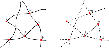
Figure 1. Left. Schematic diagram of a 3D polymer network. The curves are the polymer contours, and the red dots are the crosslinks. Right. Graph representation of the polymer network. The interconnecting polymer sections are replaced by edges and the crosslinks by the vertices.
Download figure:
Standard image High-resolution imageThe assignment of the crosslink coordinates  and the contour lengths
  is performed as follows. We begin with a
  periodic simulation box. Next,
  polymer chains, each of length
  , are placed at random inside this box. These polymers are modeled as discretized WLCs, with persistence length
  ; the discretization step-size (or bond length) is denoted by b, so each chain contains
  vertices linked by the bonds. We ignore excluded-volume interactions between bonds, and so it is fairly straightforward to 'grow' the polymers. For any polymer, the first bond
  (between vertices 1 and 2) is placed randomly in the box with random orientation. The orientation of the second bond (between vertices 2 and 3) is sampled from the probability distribution appropriate for the WLC model,
 ![$P({\hat{{\bf{b}}}}_{23})\propto \mathrm{exp}[({{\ell }}_{{\rm{p}}}/b)\;{\hat{{\bf{b}}}}_{12}\cdot {\hat{{\bf{b}}}}_{23}]$](https://content.cld.iop.org/journals/1367-2630/17/8/083035/revision1/njp517596ieqn21.gif) ,
,  , and so forth until the entire chain has been grown. Since for stiff chains (
 ), the latter probability distribution can be very narrow, we use the integral-transform method, rather than rejection-sampling, for maximum efficiency. This process is repeated for all polymer chains, after which we end up with a 'gas' of non-interacting WLC polymers (but still without crosslinks).
To introduce the crosslinks, in principle, we prepare a list of all vertex pairs. The list is sorted according to the pair separation, so that pairs with the smallest distance between the two vertices appear first. Next, the first  pairs satisfying certain criteria (soon to be prescribed) are selected from the list, and the crosslink i is placed at position
  defined to be the pair's geometric center. The set of coordinates
  thus obtained define the graph vertices. The polymer chains between the vertices define the edges of the graph, which are stored in a connectivity table. Following this procedure, each crosslink is, by means of the edges, connected to 2–4 other crosslinks (we excise all dangling polymer ends). Note that when a crosslink has only two neighbors, this implies that its connecting edges do not belong to the same filament. Indeed, the order in which the edges originating from a crosslink are stored in the connectivity table is important, as we would like to distinguish between those edges that belong to one polymer,
  , and the other edges that belong to the other polymer,
  . This distinction is needed later on to define the three-body contributions to the free-energy. Lastly, for each edge, we store the length
  of the connecting polymer chain (that is, by counting the number of vertices). Once these lengths have been stored, the graph representation is complete, after which the vertex coordinates are discarded.
The criteria, alluded to above, for the inclusion of any vertex pair as a crosslink, are as follows: (1) the vertices must belong to different polymer chains, that is, a single polymer chain is never crosslinked to itself. (2) The length of the polymer contour between two connected crosslinks may not become arbitrarily small:  . (3) Each polymer must be crosslinked at least twice. (4) No disjoint sets of vertices in the network may remain. Note that the last two criteria imply that
  cannot be chosen arbitrarily small.
2.2. Free-energy function
The total free-energy of the network is given by

where  ,
,  ,
, ![${\theta }_{{ijk}}={\mathrm{cos}}^{-1}[{{\bf{r}}}_{{ij}}\cdot {{\bf{r}}}_{{jk}}/({r}_{{ij}}{r}_{{jk}})]$](https://content.cld.iop.org/journals/1367-2630/17/8/083035/revision1/njp517596ieqn34.gif) .
.
The first term describes the two-body interactions, or pair-potentials, with the sum over all edges  in the network graph. The pair-potential is

where  is the radial end-to-end separation probability density of the WLC strand of length
  and persistence length
  connecting crosslinks i to j integrated over all orientations of both its end-tangents. Its functional form is taken from [30], which provides a good description for the tensile, compressional, buckling, and post-buckling strain regimes of a semiflexible WLC (see figure 2) within a biologically relevant range of stiffnesses.
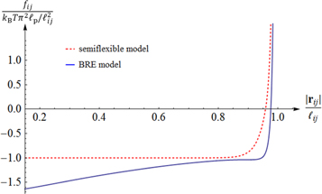
Figure 2. Typical force-extension curve of the semiflexible wormlike chain from two different interpolation formulae, namely the semiflexible wormlike chain model [29], and the Becker–Rosa–Everaers (BRE) formula [30] (which was used in this article). Here  and the Euler-buckling force is
  .
.
Download figure:
Standard image High-resolution imageThe second term in equation (1) describes the three-body interaction. In this case, the sum is over all triplets  , each representing a single polymer connecting crosslink i to j to k consecutively (with no other crosslinks in-between), and
  is the angle between
  and
and  . The idea is that the polymer backbone should persist through crosslink j and therefore penalize three-point bending between these three crosslinks. Its functional form is taken from [31]:

In a later publication, we will elaborate further on equations (1)–(3) and their interactions, particularly its underlying assumptions and the phenomenology that they neglect.
2.3. Network parameters
In what follows, we prepared our networks to mimick in vitro F-actin networks, for which the persistence length  at physiological temperatures, and the filament length is taken to be
  . The concentration of actin, defined as
  was taken to be
  , corresponding to typical experimental conditions [6, 29]. Here
  is the Avogadro constant, and
  is the typical axial separation between adjacent G-actin subunits along any strand of F-actin [32], and we chose
  , which is comparable to the size of filamin (
 ), an F-actin crosslinker [33]. We generated 20 different networks, whose parameters are listed in table 1. In the rest of this article, unless otherwise stated, all energies are measured in units of temperature
  , and all lengths in units of filament length
  .
.
Table 1.
A list of the parameters of the networks simulated for this article.  is the number of crosslinks;
  ,
,  ,
,  are the number, persistence length, and contour length of the filaments respectively;
  is the average strand length; and L is the system-size. Networks
  yielded linear shear moduli
  and bulk moduli
  . Networks 5–20 were derived by randomly removing only four-fold co-ordinated crosslinks from network 4 in order to keep
  and
and  fixed.
| Network |

|

|

|

|
L |
| 1 |

|
300 | 15.7 | 6 |

|
| 2 |

|

|
15.7 | 6 |

|
| 3 |

|

|
15.7 | 6 |

|
| 4 |

|

|
15.7 | 6 |

|
| 5–20 |
 – – in steps of 200 in steps of 200 |

|
— | — |

|
3. Nonlinear homogeneous elasticity
In order to compute the elastic response of the biopolymer network, we quasi-statically apply various linear deformations, as specified by the  deformation-gradient matrix

to the system boundary. The corresponding (Green–Lagrange) strain matrix is

where  is the affine displacement field gradient
  . (From henceforth, we will use greek indices
  to denote cartesian components, and latin indices
  to denote crosslinks.) For quasi-static deformations, the system always remains close to a free-energy local minimum. In this work, free-energy minimization is achieved numerically[34– 37].
Depending on the network reference state we desire, the minimization of the free-energy may be performed with respect to the crosslink positions alone after first fixing  , or instead, with respect to both the crosslink positions and the components
  at the same time. Both modes of minimization produce network configurations
  in mechanical equilibrium (that is, the resultant force on each crosslink at position
  is zero), with the latter mode of minimization additionally producing vanishing Cauchy stress components
  , which can be readily checked by computing the virial stress tensor [38] of the network:

3.1. Nonlinear elasticity: simulations
Starting from a reference state with vanishing Cauchy stress we apply a shear deformation

and investigate the nonlinear elastic properties of networks 1 and 2 (see table 1).
3.1.1. Shear modulus
The global elastic shear modulus  of network 2 is shown in figure 3 as a function of shear stress
  , measured in units of
  , which is the intersection between the low- and high-stress linear asymptotes of G. The linear modulus is approximately
  Pa, which is on the lower end of values reported in experiments, but agrees well with, for example, Gardel et al [6]. As has been seen in previous work [31], a strain-stiffening behavior is observed (that is, G increases with increasing stress). Loss of numerical precision prevents us from increasing shear strains beyond 0.12.

Figure 3. Superimposed plots of the second derivatives  (purple),
  (yellow), and
  (blue) for network 2 free-energy terms (that is, the two-body, three-body, and total interaction free-energies respectively) versus the global shear stress component
  induced by an engineering shear strain
  increasing in steps of 0.0001; for comparison, the affine value (green) is also shown.
Download figure:
Standard image High-resolution imageWe also split the modulus in contributions due to the three-body (bending) and two-body (compression and stretching) interactions. Interestingly, both the linear and the nonlinear response are strongly dominated by the bending mode, while stretching only contributes very little.
A bending dominated linear response is by now well understood to be due to the excitation of non-affine 'floppy' modes [8]. For the nonlinear response, previous work [9] argues in favor of a transition from such a soft nonaffine bending mode to a much stiffer affine stretching mode. The stiffening then being due to the formation of percolating paths in the tensile direction of the shear deformation. Under large enough deformation the filament strands in these paths are brought to nearly full stretching, giving rise to a modulus that diverges with stress as  [6, 7]. In contrast, here we find that the bending response itself initially dominates nonlinear behavior. To further elucidate this apparently contradictory behavior we turn to a smaller system (network 1) with
  crosslinks but with otherwise the same parameters. In this system the shear strain can be pushed to much larger values and numerics is not an issue.
In figure 4 we plot the shear modulus  of this network as a function of shear stress
  together with the contributions from bending and stretching mode. As can be seen,
  is dominated by bending at small and intermediate stresses, and by stretching only at the largest stresses. In this range, the characteristic scaling
  is observed, indicating the affine stretching of percolating paths (see figure 10 for an example of such a path). The bending-dominated nonlinear regime from figure 3 now shows up at intermediate stresses and displays a much stronger stress dependence than in the asymptotic
  regime.

Figure 4. Same as figure 4 for a network of  crosslinks (network 1) ; G is measured in units of G0 which is the horizontal low-stress G-asymptote.The buckling of a single short, or stiff, segment of the network, is responsible for the non-monotonic behavior of the G2 and G3 curves between the vertical dashed lines, and the inset is a log-linear plot showing how the corresponding 'stresses',
  and
and  , change with γ. See appendix
Download figure:
Standard image High-resolution imageBetween the low- and high-strain limits, non-monotonic changes of the two-body and three-body contributions may sometimes be also observed (as in figure 4, between the dashed vertical lines). In the case of the network sample of figure 4, this non-monotonic behavior is the response of the network to the buckling of a single short filament segment at that strain, whereupon the large local strain in the vicinity of the buckled filament causes surrounding filaments to further stretch and straighten leading to a larger increase in two-body stress and a correspondingly larger decrease in three-body stress (see the inset and the accompanying discussion in appendix
3.1.2. Normal stresses
Also of interest are the remaining components of the stress tensor  ,
,  ,
,  ,
,  , and
, and  , which are shown in figure 5 as a function of γ. We have restricted ourselves to small strains
  . Hence the normal stress components (
 ,
,  ,
,  ) are to a good approximation quadratic in the strain γ, furthermore
  and all five components are small as compared to
  —as expected.

Figure 5. Plot of the components  ,
,  ,
,  ,
,  ,
,  , and
, and  of the global virial stress tensor versus the engineering shear strain γ in network 3.
Download figure:
Standard image High-resolution imageThe normal stress components are observed to be positive, which with our sign convention, indicates that networks tend to contract when under shear deformation. This is in agreement with previous simulation results [8, 39, 40] and seems to be a general property of network-like materials [41]. The first normal stress difference  is the only other quantity (apart from the shear stress) readily accessible in cone-and-plate torsion experiments, and is directly proportional to the force exerted by the sample on the plates (for parallel-plate geometries this force is rather
  ). N1 has been reported as being negative for biopolymer networks at high strain [42]. Interestingly, in our system N1 is positive and at small strains given by
  (see inset figure 7), as expected for isotropic elastic solids [43]. Similar results were obtained in the theoretical considerations of [39], which also suggest a positive N1. There, as well as in [42], it is argued that a negative N1 in cone-and-plate geometries could be due to a relaxation of the hoop stresses (which correspond here to the
  component. A mechanism for this relaxation, however, is still elusive.

Figure 6. Nonaffinity in network 2 as a function of applied strain; yellow: total nonaffinity; blue: tensile strands only.
Download figure:
Standard image High-resolution image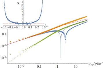
Figure 7. Stresses along the principal strain axes for simple shear. All data points refer to the simulation of network 2, while the curves are given by the weakly nonlinear model. Key: yellow squares and long-dashed curve: stress  along direction of maximum strain (extensional); blue circles and blue solid curve: stress along direction of minimum strain (compressional). Here the open circles denote negative
  , while the filled circles denote positive
  ; green triangles and dotted curve: out-of-plane stress along the z-direction. Inset: simulational data show that
  for small strains
  .
.
Download figure:
Standard image High-resolution image3.1.3. Nonaffinity
Onck et al [9] have argued that stiffening is a network property rather than a single filament property. The important network rearrangements in 2D networks are idenfied as filament reorientations (rotations) which give rise to a maximum in the nonaffinity of the response.
To quantify the nonaffinity Γ, we compute the strand length due to a small increment in strain,  and compare it to the affine value
  :
:

A plot of  versus
  is shown in figure 6 and observed to increase monotonically with applied strain. However, restricting ourselves to tensile strands only, we do indeed observe a maximum roughly at the crossover (
 ) of the modulus to nonlinear behavior. Actually,
  is negative, which indicates that strands under tension initially satisfy the demand for more strain chiefly by rotating until they can no longer do so and later resort chiefly to stretching at higher strains.
3.2. Onset of nonlinearity
As discussed in the previous section, the computed shear modulus G displays the scaling  , predicted from affine stretching of percolating paths, only at very large strains. At the onset of nonlinear behavior the modulus is still dominated by bending forces and for intermediate stresses we observe a much stronger increase of G with applied stress than expected. Both phenomena are not understood. In the following subsection, we show that generic nonlinear elasticity can account for the onset of nonlinear behavior. In the next subsection, we discuss a simple model for the orientation of fibers at high strain to explain the observed strong shear stiffening in the intermediate regime.
3.2.1. Isotropic nonlinear elasticity
When the deformation is no longer small, one has to take into account nonlinear contributions to the free energy. To analyze the onset of nonlinearities and the weakly nonlinear regime, we consider the strain energy density function of an isotropic medium, expanded in  up to cubic order:

λ and μ are the usual Láme constants from the linear theory. (Note: in this article, the symbols μ and G are often used interchangeably to denote the shear modulus.) At cubic order there are three invariants of  corresponding to three nonlinear elastic constants:
  and c3. The Cauchy stress tensor follows from equation (9) by differentiation:

We consider three simple cases: simple shear, pure shear and uniaxial extension, performing simulations in all cases with our network models, in order to determine the values of the model's elastic constants. For simplicity we always set the strain in the z-direction to zero.
Simple shear corresponds to a deformation gradient and corresponding strain tensor:

respectively. The resulting non-zero stresses are


with  . Using these equations, the values of μ,
  , and
, and  may be determined to fit the simulational data for small strains. Later, through uniaxial deformation, the the other two parameters of the model will be determined. Note from above that the relation
  holds, thus one may obtain a rough estimate of the range of γ within which this weakly nonlinear model is valid for the simulational model (see inset of figure 7). Resolving the stress tensor along the principal stretch directions, we obtain


for the normal stresses in the tensile and compressive principal stretch directions respectively. In figure 7 we compare data of the simulations for  and
and  to the simple nonlinear model equation (9). The results are seen to agree at least qualitatively; in particular the onset of nonlinearity at
  is seen to coincide with a change in sign of
  , which is compressional only for small stresses and becomes tensile in the nonlinear region. Intuitively, the sign reversal of
  suggests a tendency for the network to expand at small strains and contract at high strains for uniaxial extension, and this behavior is indeed observed in the next paragraph (see figure 8 and equation (20)). Even though demonstrating this ultimately involved the computation of an additional constant, namely c3, we note here that the form of equation (20) demonstrates that all that is required is for c3 to be positive, a property already apparent from the truncated strain energy density expansion in equation (9).
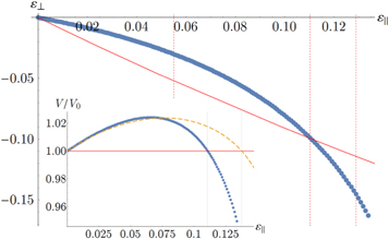
Figure 8. Transverse strain  versus longitudinal strain
  for uniaxial strain (blue data points) of network 2. The slope of the curve at
  is
is  . The red curve corresponds to the pure shear trajectory. Inset: change of total volume versus extension for uniaxial strain (blue data points) of network 2. The yellow curve is the fit given by the weakly nonlinear model equation (9).
Download figure:
Standard image High-resolution imageFor uniaxial strain we apply an extensional or compressional force in the x-direction, but allow the system to relax freely in the y-direction. The nonlinear strain is given by

with  determined from the condition of a free surface, that is,
  . During such a deformation, the volume V of the elastic material sample changes according to

where  is the initial volume in the stress-free state. Within linear elasticity, the volume change is determined by the 2D Poisson ratio
  (a constant). And from the simulations, we observe that
  (see figure 8) indicating an increase in volume for small uniaxial extension, and a decrease in volume for small uniaxial compression. For higher strains, it turns out that the nonlinear terms tend to decrease the volume (see inset of figure 8). In particular, we find

where  and
and  . Note that we have only kept the lowest order nonlinear terms in equation (20). Higher order terms are expected to limit the volume change at large strain.
Having already determined the value of μ through simple shear data, it is now possible, using the linear term of the equation above, to determine the value of λ from data on uniaxial extension. In this way we obtain the (3D) Poisson ratio  as
as  ,1
indicating a ratio of bulk to shear modulus of
,1
indicating a ratio of bulk to shear modulus of  . Combining this with the other results from simple shear, one obtains the values of c2 and
  . Furthermore, using the quadratic term of the equation above, the value of ρ may be determined from the data. This in turn enables the determination of c1 and c3, thus completing the entire set of best-fit values for the elastic parameters of the model. As a check, we perform a pure shear deformation to observe how well the determined values fit the data.
Pure shear corresponds to a deformation gradient

and strain tensor

which involves strains in the x- and y-directions such that  up to and including quadratic terms in
  . The resulting non-zero stresses are explicitly given by


The simulations show that the stress in the compressional (y-) direction of  is compressive (negative) only for small strains but then becomes tensile (positive) for large strains, which is in fair agreement with the weakly nonlinear model (see figure 9). A similar behavior is seen for the stress component in the compressional direction for simple shear (see figure 7).
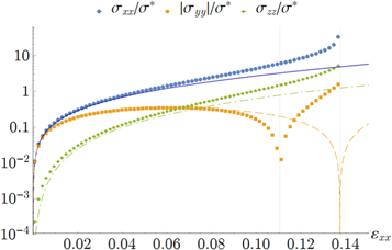
Figure 9. Stress components along the x, y, and z axes for pure shear of network 2. Data points correspond to the simulations, while the smooth curves are given by the weakly nonlinear model using values of elastic parameters λ, μ, c1, c2, and c3 predetermined from simple shear and uniaxial extension.
Download figure:
Standard image High-resolution imageIn summary, the weakly nonlinear model demonstrates that (1) it is possible to obtain a volume-change sign-reversal for large enough uniaxial strains, even for positive c1, c2, and c3, and (2) that once the relevant parameters of the model have been determined through fitting with data, it is also able to predict changes of the sign of stress in other deformation types, such as the normal stress in pure shear, for example.
3.3. Reorientation of fibers at high strains
As the nonlinearities become more prominent, the above expansion ceases to be applicable. Besides the strength of the deformation which becomes too large to be treated perturbatively, it is the assumption of isotropy which breaks down at large strain. To illustrate this point, we highlight in figure 10 the force chains under the highest tension (in red) as well as the strands which sustain high compressional forces (in green). For such large shear deformations the stretching of single fibers gives rise to the known scaling,  . In this section, we propose a simple toy model to account for the comparatively faster rate of stiffening observed before the asymptotic scaling is reached. The basic mechanism under consideration is the rotation of fibers or segments into the tensile direction. In the simplest version we model the strands as inextensible, but extensibility can be taken into account easily.
For simplicity, we will focus instead on the scaling dependence of the Young's modulus  on uniaxial stress
  at intermediate values of stress. Here,
  is the scaling exponent. Figure 11 shows how in our simulations
  changes with
  . As expected, at low values of
  , the scaling is linear, and
  . At intermediate values of
  may rise to a maximum which can be as high as five, before at last falling to a value of
  which indicates that a few strands (forming a force-chain percolating the network, as in figure 10) are being stretched affinely and are dominating the stress. The non-specific value for the maximum of
  hints at an exponential regime at intermediate stresses.

Figure 10. For large shear deformations, even though the network still looks geometrically isotropic, in a mechanical sense, it is not. As shown in this simulation snapshot of network 1 (with periodic boundaries), a force-chain under the highest tensions appears along the principal stretch-direction (signified by the thickest red strands) and dominates the stress along that direction, while a number of strands along the principal compression-direction sustain large compressive forces (signified by the thickest green strands). A large number of strands mediate comparatively small forces (these are dimmed out in the figure in order to highlight the largest forces).
Download figure:
Standard image High-resolution image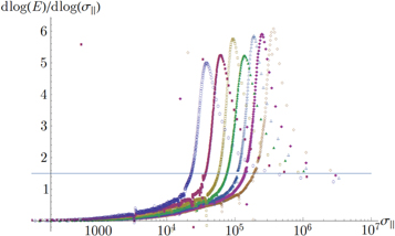
Figure 11. A linear-log plot of the scaling exponent  of Young's modulus E versus uniaxial stress
  for networks 8, 10, 12, 14, 16, 18, 20 with
  , 5800, 6200, 6600, 7000, 7400, 7800 (counting from left to right) all of which use the same set of filaments.
Download figure:
Standard image High-resolution imageIn order for percolating tensile paths to be formed, filaments or parts of filaments (strands) have to align themselves with the tensile direction. Note that not all strands of the network will eventually be aligned with the tensile direction, otherwise the lengths of those network dimensions transverse to the tension would collapse to zero at full alignment, which is not what is observed (see figure 10). It turns out that we can understand the exceptionally strong stiffening in the intermediate nonlinear regime via this mechanism of filament alignment. To this end, consider an inextensible strand of length  oriented at a force-dependent angle
  to the tensile direction. Changing the pulling force
  f gives rise to a differential torque
  , which tries to rotate the filament even further,
  , where
  is an effective material-constant that, for simplicity, we take to be constant and independent of the pulling force. It plays the role of the (bending dominated) linear modulus
  .
.
Thus, we obtain the following differential equation:

which can be integrated to give

where  is the initial orientation of the strand. The crucial aspect is the exponential dependence on force
  . The strain
  can be computed from the average
  , where the average is over the initial angles
  of the strands in the percolating path:

For strongly aligned strands, we approximate  and compute

resulting in an exponentially increasing modulus  . Note that the argument here is asymptotic, and one might expect this behavior to carry over to the shear modulus as well. But in simple shear, an additional complication arises, namely, compression is applied along one-dimension transverse to the maximum strain in order to keep
  constant. Extending the above argument to include this extra behavior is nontrivial and will be the subject of another article.
Similar exponential stiffening has been reported in [46] in the context of a network of rigid rods crosslinked by flexible linkers. The authors present an alternative explanation that is based on treating the flexible linkers as an effective elastic medium [47].
3.4. Variation of network parameters
To check the robustness of the intermediate regime against parameter variations we varied the average strand length  , i.e. the average distance between consecutive crosslinks along filaments. With the overall filament length fixed, a smaller strand length means more crosslinks per filament. This increases the modulus,
  , as can readily be seen in figure 12. Such a variation is in agreement with the theory of non-affine floppy bending modes [14, 22] of wavelength
  b and amplitude
  independent of
  . The resulting modulus then is given by
  , where the first factor is the spring constant of the bending mode, the second accounts for the number of strands per filament, and
  counts the number of filaments in the volume
  . For the nonlinear response we observe that the onset of intermediate exponential stiffening is shifted to smaller stresses in the weakly crosslinked networks. This indicates that reorientation effects are stronger in weakly crosslinked networks, thus filaments are more easily rotated when not highly crosslinked to its neighbors.
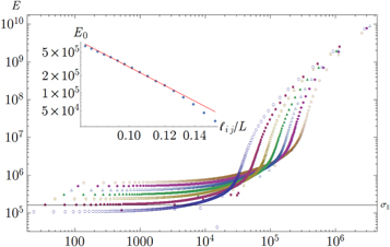
Figure 12. Young's modulus  versus stress
  for different average strand lengths
  . Inset. Scaling of linear modulus
  as a function of average strand length
  . The slope of the line is −4. The networks considered here are the same as for figure 11.
Download figure:
Standard image High-resolution image4. Local elastic constants
Until now, the aforementioned elastic quantities, such as stress and strain, have all been macroscopic quantities, referring to the system box as a whole as if it were a homogeneous continuum. Even though, through free-energy-minimization, they correctly account for the non-affine response of the network, they reflect little of the elastic heterogeneity within the network. However, these elastic heterogeneities are relevant for many reasons. When a biopolymer network ruptures, e.g. under the action of motors, a particularly weak spot is expected to give way first. Many cell functions require the formation of protrusions, which possibly make use of locally weak regions in the cytoskeleton. Furthermore, microrheology experiments in networks and cells measure the local elastic properties, and hence need to be interpreted in terms of fluctuating elastic constants.
Being essentially a discrete system, the network's elastic heterogeneity is not trivially described using continuum elasticity theory. Indeed, in order to characterize the heterogeneity of the network we resort to a well-established formalism of local continuum elasticity which employs a form of spatial averaging around any observation point  , over a chosen length-scale—the coarse-graining width
  —while adhering to physical conservation laws, such as the conservation of matter, momentum and energy. A suitable coarse-graining probability density distribution
  may be chosen to provide the necessary weights for the averaging. In this work, we choose
  . To avoid repeating a long discursion of the theory leading up to the salient results, we refer the reader to s [38, 48] for a thorough ab initio treatment. Also, the formalism used here has already been employed in simulations of the elasticity of glasses or amorphous solids consisting of particles interacting via a Lennard–Jones potential [11, 12, 49]. In the rest of the article, we use the terms 'global' and 'local' to distinguish between the homogeneous and heterogeneous elastic quantities respectively.
4.1. Coarse-graining
In appendix  -body interactions the often-quoted local stress tensor for pairwise interactions. The point-wise local stress for the networks of this article (which have only two- and three-body interactions) is therefore

where

and

The sum in equation (31) is over all filament segments  j (that is, the edges), and the sum in equation (32) is over all bending angles i
  but allows for all 3 permutations of the dummy indices
  are two-body and three-body forces defined in appendix

where the point-wise coarse-grained local linear displacement is

Here  is the displacement of the
  th crosslink after a (global) deformation specified by, say
 ![$[{\Lambda }_{\alpha \beta }]$](https://content.cld.iop.org/journals/1367-2630/17/8/083035/revision1/njp517596ieqn227.gif) , has been applied to the system-boundary and the network subsequently minimized.
, has been applied to the system-boundary and the network subsequently minimized.
In figure 13
we show the distribution of local stress-component  in a reference state without global prestress. These data demonstrate that on a local scale the network is strongly prestressed, giving rise to a broad distribution of local stresses. The width of the distribution shrinks as a function of growing coarse-graining length as one would expect.
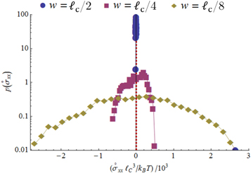
Figure 13. Log plot of the probability distribution of local stress component  at different coarse-graning length scales
  . The data refer to network 2 at zero global stress.
Download figure:
Standard image High-resolution imageOne final remark concerns the range of coarse-graining lengths accessible to our simulational data. The computation of local stresses and strains requires at least two mass points. Hence the coarse-graining scale should be larger than the distance between two 'particles', or crosslinks. This limits us to  .
.
4.2. Local elastic constants in a prestressed state
We have seen in the previous section that the network supports considerable stresses on a local scale. In order to compute the local elastic constants, we thus need to consider a prestressed reference state. In the following, we will ignore crosslink positions, assuming that they are always at their equilibrium positions, and denote a reference state simply as  with a generally non-vanishing stress
  and volume
  . We will apply an additional deformation
  to compute the elastic response of the reference system. (Note that an observable
  in the reference state is denoted by
  .)
.)
The stiffness of any state of the system is described most generally by a fourth-order modulus tensor  defined by [50]:


where  is the second Piola–Kirchoff stress tensor written as a function of
  . Consequently,
  possesses the following symmetries:
  amounting to 21 independent components in general. In simulations of random polymer networks, it is common to assume elastic isotropy of the network and accordingly compute only 2 elastic constants: namely the bulk modulus
  and the shear modulus
  of the network. However, this assumption is true only in the thermodynamic limit for unstressed networks. Thus in our investigations of local moduli, we choose to maintain the most general symmetry possible in continuum elasticity, namely, the triclinic symmetry, and observe how this symmetry tends to isotropy (or some other symmetry) as the system-size or coarse-graining scale increases (while keeping the intensive properties of the system constant).
It has been shown [50] that the Cauchy stress in the new reference configuration  is to first-order given by

Writing  , where
  are the symmetric and anti-symmetric parts of
  respectively, it follows that

in tensor notation. (If there is little pre-stress [ ], all the terms after the first term on the left-hand side of equation (37) may be taken to vanish. For this reason, these terms have often been neglected in simulations of glasses [12], where the so-called 'quenched stresses' are small.)
Our starting point is equation (37) which we apply locally at any observation point  . The local coarse grained displacement field
  is in general non-affine and given, to linear order, by equation (34). For small global strains, the local linear strain
  due to
  is expected to approach the global strain
  as the coarse-graining scale
  increases, approaching the system size and beyond (see figure 13). Indeed, since
  ,
,  , and
, and  are all readily computable from the microscopic coordinates
  via equations (31), (33) and (34), one may use equation (37) to solve for
  . The method proceeds as follows: for any reference state
  of the network, we apply six small homogeneous deformations
  along the six possible linearly independent directions of the strain tensor, and minimize with respect to the crosslink coordinates in order to obtain six different states
  . That is, for each deformation we set
  where all the components
  are zero except for one which is very small in value (see table 2 for detailed information).
Table 2.
List of the six linearly independent deformations used in this article to compute the elastic modulus tensor. The other three components of  , that is,
  , and
, and  were set to 0 for all
  .
.
| Deformation d |

|

|

|

|

|

|
|---|---|---|---|---|---|---|
| 1 | 1 | 1 | 1 | 0 | 0 |

|
| 2 | 1 | 1 | 1 | 0 |

|
0 |
| 3 | 1 | 1 | 1 |

|
0 | 0 |
| 4 | 1 | 1 |

|
0 | 0 | 0 |
| 5 | 1 |

|
1 | 0 | 0 | 0 |
| 6 |

|
1 | 1 | 0 | 0 | 0 |
At any observation point  , the local stress
  before deformation and the local quantities
  ,
,  , and
, and  after each of the six deformations are computed. The local modulus at any observation point
  may then be computed as follows: using equation (37) six times (one for each deformation), an overdetermined system of 36 linear equations in 21 unknowns (the components of the local modulus tensor) is obtained. This number of equations should be reduced, through careful selection (see, for example appendix
  may be computed at observation points
  located at the nodes of a regularly spaced grid of points within the system box. A similar procedure may be employed to determine the global modulus tensor defined in the previous subsection: in this case, it is perhaps simpler to directly use equation (36), instead of equation (37), with the replacements
  , since it is known [51] that

where the global Cauchy stresses  may be obtained using equation (6).
4.3. Anisotropic elasticity
A particular linear combination of the 21 elastic constants gives the so-called 'best isotropic approximation' [52, 53]  to the modulus tensor
  , yielding an approximate shear modulus
  and bulk modulus
  , whose expressions are given in appendix
  , called the 'index of anisotropy', measuring how far the system is from isotropy, is also defined [52].
  ranges from 0 to 1, and it vanishes for a completely isotropic medium. Note that in our computational models even the global moduli are anisotropic due to finite system size.
In figure 14 we show the average index of anisotropy as a function of coarse-graining length for two sizes of networks. The figure demonstrates that the network is isotropic in the thermodynamic limit, but anisotropic on a local scale and in small networks. For the larger network ( ), the index of anisotropy
  for a coarse-graining scale comparable to the mean distance between crosslinks and
  0.1 for a coarse-graining scale comparable to the filament length. These are the length-scales, where we expect to see fluctuations in the moduli, as discussed in the next paragraph.
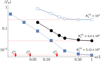
Figure 14. Log–log plot of the mean local index of anisotropy  versus the coarse-graining length
  for three network realizations all of the same crosslink and polymer densities, but of increasing system-size (networks 1–3). The red arrows mark the values of
  for the respective networks.
Download figure:
Standard image High-resolution image4.4. Elastic inhomogeneities
The distribution of local bulk modulus is shown in figure 15 for five values of coarse-graining length. As expected, the distributions become sharp as the coarse-graining length approaches system size. This limiting behavior is quantified by plotting the variance relative to the mean as a function of  , as done in the inset of figures 15.
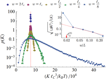
Figure 15. Log plot of the probability distribution of local bulk modulus  (obtained using the best isotropic approximation) at different coarse-graning length scales
  . The red vertical dashed line marks the global value of
  . Inset: log plot of the standard deviation of
  . The red line denotes the trend that would be expected from the central-limit theorem, and its slope is
  . Both figures refer to network 3.
Download figure:
Standard image High-resolution imageThe fluctuations of the shear modulus are strongly correlated with the fluctuations in the density. The correlation factor is

for all coarse-graining lengths. (Here  .)
.)
Next, we check the dependence of the elastic heterogeneity on degree of crosslinking. Reducing the number of crosslinks by roughly  from the initial value (six crosslinks per filament), the network loses its stiffness towards shear deformations. The variance is similarly decreasing in this range of
  so that the variance relative to the mean is approximately independent of crosslink concentration. On the other hand, the elastic heterogeneities increase with increasing shear stress as can be seen in figure 16, where we plot the variance relative to the mean a a function of stress

for several coarse graining lengths. Naturally the variance strongly decreases with coarse-graining length, as the local modulus approaches the global value.
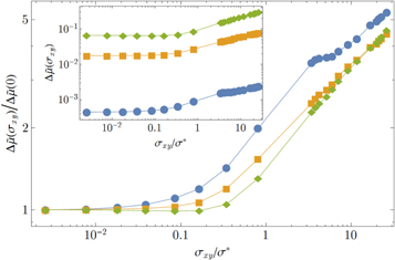
Figure 16. Log plot of the variance of the local shear modulus of network 2 as a function of stress for four coarse-graining lengths  corresponding to the symbols
  ,
,  ,
,  respectively.
Download figure:
Standard image High-resolution imageWe expect the nonaffine deformations to be correlated with the fluctuations in the elastic constants, such that hard regions suppress the deformation below the affine value, whereas soft regions allow for deformations larger than the affine value. However, we only find a very small effect, when quantifying these correlations.
Defining hard (soft) regions as those whose local modulus exceeds (falls below) the mean, one may alternatively look at distributions of nonaffine displacements for the soft and hard regions separately as suggested in [12]. The normalized distributions are shown in figure 17. Clearly the large displacements are significantly more probable in soft regions.

Figure 17. Log–log plot of the distribution of displacements transverse to the affine ones; the blue circles mark the soft regions and the red squares mark the hard regions; the coarse-graining length was chosen comparable to the mesh-size, that is, the mean distance between crosslinks. The network referred to here is network 2.
Download figure:
Standard image High-resolution image
5. Conclusion
We have studied the elasticity of filamentous cytoskeletal networks. These networks cannot be described as homogeneous elastic materials. The constituting filaments are elastically anisotropic, with a small bending and a high stretching stiffness, dominating the response ar small, respectively large applied strain. Networks are heterogeneous, they have a broad pore-size distribution and are hierarchical with several length-scales ranging from microscopic to 'mesoscopic' scales defined by the filament length, exceeding the scale of the pores.
In this work, we focus on two aspects of network elasticity: the crossover between linear and stretching dominated elasticity and the occurrence of elastic heterogeneities, i.e. elastic properties that are not spatially constant but vary across the system.
The onset of nonlinear behavior is consistent with generic nonlinear elasticity theory which, using only considerations of isotropic symmetry up to quadratic order in the constitutive relations, makes certain nontrivial mechanical phenomena possible such as those displayed by our simulations, namely: (1) the first normal stress difference in simple shear,  up to and including terms of
  . (2) For isochoric deformations, the stress in the maximum compressional direction of the strain tensor is compressional only in the linear regime but becomes tensile for larger strains. This result holds for simple as well as pure shear. (3) Correspondingly, the volume change for uniaxial extension is positive in the linear regime only and negative for larger strains.
Even though it is well known that the asymptotic behavior for large strain is stretching dominated, we observe strongly nonlinear behavior already in the bending dominated regime. A simple model for the orientation of fibers gives rise to an exponential increase of the modulus, a result which is supported by our simulations.
To study elastic heterogeneities, we provide a coarse-graining scheme that sets the scale of interest and allows us to calculate local versions of stresses, strains, and elastic moduli. We calculate the probability distributions of stresses and elastic moduli as a function of coarse-graining width. On a local scale, networks are generally at finite stress, even though we prepare the networks with a vanishing stress tensor on the macroscopic scale. Moreover, all (nominally isotropic) networks are locally anisotropic, with a maximum number of non-vanishing moduli. This elastic anisotropy persists to the macroscopic scale in finite-sized systems and vanishes only in the thermodynamic limit.
The relative fluctuations of the moduli are largely independent of crosslink number but increase significantly in the nonlinear regime. We also study the correlation functions of the local moduli and show that local stiffness is highly correlated with local density.
Our work provides a basis for more realistic modelling of biopolymer networks. It is straightforward to generalize the approach to bidisperse networks of say actin filaments together with microtubules. It is also possible to incorporate active elements. We plan to study the dependence of elastic properties on molecular motor activity. More advanced questions to be addressed are shear-stiffening due to internal stresses, dominance of contractile forces, violation of the fluctuation-dissipation theorem, and possibly the rupture of networks due to molecular motor activity.
Acknowledgments
CH would like to acknowledge DFG via Emmy Noether grant He 6322/1-1. RLCV would like to acknowledge Emmy Noether Vi 483. Financial support by the Deutsche Forschungsgemeinschaft through Grants No. SFB-937/A1, A10 and A16 is gratefully acknowledged.
Appendix A.: Two- and three-body stress contributions
The following discussion attempts to explain the sharp variation of the curves in the inset of figure 4. The derivatives of the two-body and three-body free-energy densities with respect to the shear strain are
which, in the limit of  become


where  and
and  are respectively the two-body and three-body contributions to the Cauchy stress. Here, we have, for convenience, employed the so-called 'reduced coordinates'
  [54] of the real-space positions of the crosslinks.
Note also that the  (as do their real-space counterparts
  ) always minimize the total free-energy
  . Therefore both
  and
and  are, in fact, affine contributions. The extra terms in equations (A.1) and (A.2) are the non-affine contributions. It can be shown that the condition of mechanical equilibrium
  implies

Thus

which is the Cauchy shear stress.
Whenever any filament-segment, say  , undergoes buckling during the shearing process, the second term in equation (A.1) becomes overwhelmingly dominated by the large change in end-to-end separation of that segment with strain:
  . Thus, the second term in equation (A.1) becomes responsible for the sharp variation of the bottom curve in the inset of figure 4. (See also the animations provided as Supplementary Information accompanying this article.) Accordingly, the second term of equation (A.2) undergoes an equally large but opposite variation since the condition of mechanical equilibrium constrains the sum of this term and the second term of equation (A.1) to vanish, resulting in the relatively featureless monotonic behavior of the Cauchy stress
  (the top curve in the inset of figure 4). This argument may be extended to the second derivatives of the two-body and three-body interactions in order to explain the non-monotonic behavior in the curves G2, G3, and G of figure 4 itself.
Appendix B.: Local stress for n-body interactions
Here we extend the derivation of the two-body collisional stress tensor, which has been outlined in [38, 48], to n-body interactions. From Glasser and Goldhirsch [48, equation (30)], the time-rate of change of the local coarse-grained momentum density at the point  within an N-particle medium, relevant for quasi-static deformations, is given by

where  is the total force on particle i whose position is
  , and
, and  is the coarse-grained density function normalized to 1 over all space and with a single maximum at
  . Suppose that the inter-particle interactions are due to a sum of n-body potentials—that is, the potential energy of the system is

Then
where

Next, we make use of a generalization of Newton's third law which can be readily shown to be true for systems of particles that interact only with each other:
This equation is in fact a consequence of the translational invariance of the potential energy in equation (B.2). Thus for any α we may write
Thus equation (B.1) becomes
Choosing  guarantees that for each term in the third summation, there is a corresponding one in the second summation. So that after rearranging dummy indices we can rewrite
where, in the last equation, we have used the identity:

Finally, using equation (B.1), we identify the tensor

as the local coarse-grained stress tensor for n-body interactions. For  , we have

(which is identical to that derived in [48] for pairwise interactions), and
For completeness we include the full expression for the stress tensor:

Appendix C.: Elastic constant computation
The linear system of equations to be solved is derived from six independent homogeneous deformations, each of which uses an equation of the form  (see equations (36) and (37)) to yield a set of six linear algebraic equations with the 21 elastic constants
  as variables to be solved for.
The system of equations for the d-th deformation is here displayed in the so-called Voigt notation:
In order to solve for the elastic constants  , the over-determined set of 36 linear equations obtained must be reduced to a set of 21 linearly independent equations. Assuming none of the strain components vanish, we selected all six equations of the first deformation, the first five equations of the second deformation, the first four equations of the third deformation, and so on. This procedure yielded one such set of linearly independent equations. These equations were then solved using a sparse-matrix numerical solver to obtain the elastic constants.
For the case of the homogeneous moduli, our particular choice of six homogeneous deformations (see table 2) causes most of the components of the strain to vanish. It is then easy to show that the modulus matrix in Voigt notation is (compare its components with corresponding components in the modulus matrix in equation (C.1))

Appendix D.: The best isotropic approximation
The bulk and shear moduli are linear combinations of the components of the modulus tensor:


See, for example, references [52, 53] for a derivation of these formulae. In brief,  is the projection of
  from the space of modulus tensors onto the space of isotropic modulus tensors [52]. It turns out that these same estimates may also be obtained by isotropically averaging the modulus tensor [53]. The index of anisotropy is

where the tensor norms ![$\parallel [{C}_{\alpha \beta \gamma \delta }^{\mathrm{iso}}]\parallel $](https://content.cld.iop.org/journals/1367-2630/17/8/083035/revision1/njp517596ieqn344.gif) and
and ![$\parallel \;[{C}_{\alpha \beta \gamma \delta }]\;\parallel $](https://content.cld.iop.org/journals/1367-2630/17/8/083035/revision1/njp517596ieqn345.gif) are
are

Footnotes
- 1