


Abstract
We investigate the physical origin of the existence or absence of Dirac cones in graphynes by combining first-principles calculations with the downfolding method. We clarify that acetylenic linkages (−C≡C−) can be reduced into an effective hopping term between vertex atoms, and thus various graphynes may be described by a unified tight-binding model on a honeycomb lattice, which is topologically equivalent to that of graphene. Critically, whether Dirac cones exist or not in graphynes is determined by the combination of hopping terms. Based on the unified model proposed, two additional graphynes are revealed to possess Dirac cones, one of which has a rectangular symmetry and contains only four vertex atoms in a unit cell.
Export citation and abstract BibTeX RIS

Content from this work may be used under the terms of the Creative Commons Attribution 3.0 licence. Any further distribution of this work must maintain attribution to the author(s) and the title of the work, journal citation and DOI.
1. Introduction
The occurrence of Dirac cones is a peculiar phenomenon in band structures where the valence and conduction bands meet at a single point at the Fermi level, forming a double cone with a linear dispersion in the vicinity. The Dirac cones in graphene were first predicted by Wallace [1] in 1947 in the context of a tight-binding (TB) approximation and have attracted much interest in recent years after they were experimentally observed by Novoselov et al in 2005 [2]. The most interesting aspect of the Dirac cones in graphene is that the low-energy excitations are massless chiral Dirac fermions, which have unusual tunneling and transport properties and play a role in the quantum Hall effect [3, 4]. This unique band structure of graphene was widely believed to be a consequence of its hexagonal honeycomb structure. However, it has been noted that the Dirac cones of graphene are preserved under an applied strain (which breaks the rigorous hexagonal symmetry), even though the Fermi points are shifted away from the K points [5, 6]. Dirac cones have also been observed in rhombohedral graphene antidot lattices [7] and strongly bound graphene systems [8]. These results imply that a rigorous hexagonal symmetry is not a requisite for Dirac cones to exist in two-dimensional carbon allotropes. Some effort has gone into exploring the possibility of existence of Dirac cones in systems other than graphene [9–19]. Recently, Malko et al [10] found that Dirac cones also exist in graphynes, which are the carbon allotropes composed of sp- and sp2-bonded carbon atoms, where one of these graphynes has a rectangular instead of a hexagonal symmetry. This has raised an intriguing question about the relationship between the existence of Dirac cones and the symmetry of the materials in which they are found.
Graphynes may be viewed as the result of replacing some single bonds in graphene with acetylenic linkages (−C≡C−) [20]. Despite their similarity to graphene in topology, graphynes exhibit diverse electronic properties: some graphynes are semimetals with Dirac cones [10, 14, 15], while others are semiconductors [9, 14, 15, 20]. Kim and Choi [14] have conceptually showed that the acetylenic linkages can be simplified into single bonds with a renormalized hopping parameter, which was supposed to play an important role in determining the electronic properties of graphynes. Liu et al used a TB model with three independent parameters to fit the electronic structure of a few graphynes well and thus verified the validity of the TB model in graphyne studies [15].
In this paper, we investigate the electronic structure of graphynes by combining first-principles calculations with the downfolding method. We demonstrate that all graphynes (including those with a rectangular symmetry) are topologically equivalent to graphene and may be described by a single unified model. In addition, we presented two more graphynes with Dirac cones, one of which also has a rectangular symmetry.
2. Methods
First-principles calculations were performed within the framework of density functional theory as implemented in the QUANTUM ESPRESSO package [21]. A kinetic-energy cutoff of 100 Ry was used for the plane-wave expansion of the valence wavefunctions, and we adopted a generalized gradient approximation with the Perdew–Burke–Ernzerhof exchange correlation functional [22]. The core–valence interaction was described by means of the Vanderbilt ultrasoft pseudopotential [23]. All structures were fully relaxed with a convergence tolerance of 10−4 Ry au−1 for atomic forces. We obtained the self-consistent ground state using a 21 × 21 × 1 Monkhorst–Pack mesh of k-points [24] and a fictitious Fermi smearing of 0.005 Ry for the Brillouin-zone integration.
After obtaining the self-consistent ground state of graphynes, we used the WANNIER90 package [25] to construct real-space maximally localized Wannier functions (MLWFs), and to express the Hamiltonian in the basis of MLWFs to build the full TB model where we neglected long-distance hopping terms. The initial guess for iterative MLWFs minimization was based on atom-centered sp2, pz and triple-bond orbitals. The full TB model was then reduced by the downfolding method to produce an effective TB model that contains only vertex pz orbitals.
3. Results and discussion
3.1. Analysis from maximally localized Wannier functions
We first analyze the bonding character and electronic structure using MLWFs, which may serve as ideal building blocks in models for the electronic structure of nanostructures [26]. In contrast to graphene, there are both sp and sp2 hybridized carbon atoms in graphyne, resulting in different bonds [27, 28]. Figure 1 summarizes the MLWF analysis for α graphyne, as a typical example of various graphynes. Each vertex atom exhibits sp2 hybridization with neighboring atoms to form three σ bonds (figure 1(a)), which correspond to deep valence bands. Because of the tetravalent nature of C, the pz orbital of vertex atoms forms a localized π orbital (figure 1(b)), which constitutes the main component of bands near the Fermi level. The triple bonds in acetylenic linkages are represented by three MLWFs (figure 1(c)), lying between two sp C atoms that are distinguished by a 120° rotation. It is therefore straightforward to express the Hamiltonian in the basis of the MLWFs from figures 1(a)–(c) and then to re-calculate the band structure, i.e., to make the Wannier interpolation with restricted basis. A comparison of the direct first-principles results and the Wannier interpolation is shown in figure 1(d), where we see excellent agreement. The massless bands near the Fermi level are reproduced quite well, vindicating the choice of MLWFs in the analysis.

Figure 1. Electronic properties and geometry of α graphyne. (a)–(c) Isosurface contours of various MLWFs (red for positive values and blue for negative): (a) σ bonds, (b) pz orbitals and (c) triple bonds. (d) The band structures from first-principles calculation and Wannier interpolation. (e) The atomic structure and the effective model.
Download figure:
Standard image3.2. Effective Hamiltonian
As described above, when expressed using a basis of selected MLWFs, the Hamiltonian reproduces first-principles results quite accurately. Because of the strong localization of MLWFs, the matrix elements of two MLWFs decay rapidly with increasing distance between them, and by neglecting long-distance hopping terms, a TB model can be constructed [29]. A graphyne model obtained in this way contains a large number of MLWFs. However, we can adopt further approximations to reduce the TB Hamiltonian and facilitate the analysis. Some MLWFs have deep energy levels: the σ bonds for example (figure 1(a)) are characterized by a very low on-site energy (∼12 eV below the Fermi level), so they can be safely cast. An additional approximation is derived from the observation that the main contributions to bands near the Fermi level come from the pz orbitals of vertex atoms. This implies that an ideal construction involves an effective TB Hamiltonian containing only vertex pz orbitals. However, in graphynes, electrons from one pz orbital can hop to another pz orbital either directly or through other MLWFs (such as found in triple bonds). Between pz orbitals separated by acetylenic linkages, direct hopping of electrons is negligible, and indirect hopping is dominant. To construct the effective Hamiltonian that considers this indirect hopping process, we made use of the downfolding method, as briefly explained below.
The downfolding method is also known as a matrix condensation or Shur complement. It is an effective way to derive a few-band Hamiltonian from first-principles results with 'complete' MLWF basis [30, 31]. The method yields a minimal basis set from a large set of MLWFs by integrating out the other degrees of freedom. In the example of graphynes, their MLWFs may be divided into two parts: the vertex pz orbitals, {Ψπ}, which form the main components in the spectrum near the Fermi level; and the remainder of MLWFs, {ΨTri}, which are mainly the triple-bond orbitals. The Schrödinger equation takes the form


where Hπ(Tri),π(Tri) are the blocks of the Hamiltonian matrix and E is the eigenenergy. One can solve for |ΨTri〉 in (2)

and substitute the result into (1), yielding an equation for |Ψπ〉:

The contents inside the square brackets can be regarded as an E-dependent Hamiltonian, which has to be determined self-consistently. Since we are only interested in the spectrum near the Fermi level and the on-site energy of {ΨTri} (the diagonal elements of HTri,Tri) lies far from the spectrum of interest, (4) can be approximately written as

where EF is the Fermi level. Thus, we obtain an effective Hamiltonian for the minimal orbitals of {Ψπ} (assuming that EF = 0)

Based on the first-principles calculation of α graphyne, the blocks of the original Hamiltonian matrix containing two vertex atoms and an acetylenic linkage are given by


where e0 = −2.66, e3 = −6.17, t0 = 0.32, t3 = 3.55, and t = 1.11 (all in eV). The third triple-bond MLWF (see figure 1(c)) is perpendicular to pz orbitals, so the hopping terms between them are zero, as shown in (9). The effective Hamiltonian for two vertex pz orbitals separated by an acetylenic linkage can be denoted as

Then the effective hopping between neighboring pz orbitals via an acetylenic linkage,  , can be deduced analytically from (6)–(9) to be

For α graphyne, it was determined that  eV. It is noted that, in comparison with the approach adopted by Kim and Choi [14], the exact value of the effective hopping parameter can be determined from first-principles calculations in the current scheme as described. Our approach also differs from what was adopted by Liu et al [15] where on-site energy was supposed to be zero at all C atoms. After this downfolding process, the effective Hamiltonian for α graphyne is almost identical to that of graphene except that the hopping parameter takes different values. This sheds light on the facts that the band structure of α graphyne is very similar to that of graphene and that their Dirac points are located at the same K and K' points as graphene [10].
3.3. Existence/absence of Dirac cones in graphynes
Since the major effect of acetylenic linkages is to mediate the effective hopping terms between vertex pz orbitals as described above, all graphynes may be described in a unified scheme in which pz orbitals reside at vertices of a honeycomb lattice, and electrons hop from one vertex to its neighboring vertices as described by two kinds of hopping terms: one is for the hoppings between vertices separated by acetylenic linkages, denoted as  as described above; and the other is for direct hopping between vertices that are connected by single bonds, which we therefore denote with td. Different combinations of such hopping terms describe different graphynes, giving rise to the existence or absence of Dirac cones.
As was previously discovered [10, 14, 15, 20], β graphyne is a semimetal with Dirac cones, while γ graphyne is a semiconductor (figure 2). Both β and γ graphynes (and even α graphyne) can be described by a common model composed of a  supercell and a hopping pattern as shown in figure 2(d). In this hopping pattern, 1/3 of hoppings belong to one class (tr, represented by red edges in the figure) and 2/3 of hoppings belong to the other class (tb, represented by blue edges). For α graphyne, both red and blue edges represent indirect hopping (
 ). For β graphyne, red edges represent direct hopping (td), while blue edges represent indirect hopping (
 ) (figures 2(c), (d)), where the situation is reversed for γ graphyne (figures 2(d), (e)). From our analysis in appendix A, the criterion for the existence of Dirac cones in the common model of figure 2(d) is given by the satisfaction of either of the following:

or

The indirect and direct hopping parameters derived from first-principles calculations for various graphynes are summarized in table 1 together with the original elements in MLWFs. It is determined that tr/tb = 1 for α graphyne and  for β graphyne, which satisfy (12) and (13), respectively. For γ graphyne, however,
  , satisfying neither (12) nor (13). This explains why Dirac cones are found to exist in α and β graphynes, but not in γ graphyne. It is interesting that, although the effective hopping parameters obtained by Liu et al [15] are different from ours (because different TB models and renormalization procedures were used), the application of the current criterion on their data also arrives at the same conclusion. In addition, the analytic solution predicts that the Dirac cones are located at the Γ–M lines (see appendix A), consistent with the first-principles calculations in figures 1 and 2 (noting that the K and K' points for α graphyne fold to the Γ point if the same supercell with six vertex atoms were adopted).
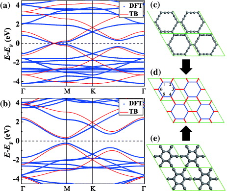
Figure 2. Properties of β and γ graphynes. (a), (c) The band and atomic structures of β graphyne. (b), (e) The band and atomic structures of γ graphyne. The band structures from first-principles calculations are depicted in blue dotted lines, while those from the effective TB model are depicted in red solid lines. (d) Schematic illustration of the effective TB model with two kinds of hopping terms (represented by red and blue edges). Six vertex carbon atoms in (d) are labeled with numbers from 1 to 6.
Download figure:
Standard imageTable 1. The TB Hamiltonian matrix elements obtained by MLWFs and the downfolding method (in units of eV).
| e0 | t0 | t | e3 | t3 | td |
 |
|
|---|---|---|---|---|---|---|---|
| α graphyne | −2.66 | 0.32 | 1.11 | −6.17 | 3.55 | – | 1.25 |
| β graphyne | −2.18 | 0.36 | 1.22 | −6.14 | 3.57 | −1.79 | 1.52 |
| γ graphyne | −1.66 | 0.45 | 1.30 | −6.19 | 3.59 | −2.11 | 1.74 |
| 6,6,12-graphyne | −1.53 | 0.48 | 1.26 | −6.02 | 3.56 | −2.05 | 1.76 |
Another interesting example is found in 6,6,12-graphyne. It does not have a hexagonal symmetry, but it also possesses Dirac cones in the band structure [10]. According to the effective TB model derived previously, 6,6,12-graphyne (figure 3(a)) should be equivalent to a system on a honeycomb lattice with rectangular supercells containing eight vertices (figure 3(b)). In other words, although 6,6,12-graphyne has a rectangular symmetry, its TB topology is equivalent to that of graphene. The resemblance between 6,6,12-graphyne and graphene is also demonstrated by comparing their band structures where the same supercell is adopted in graphene (figure 3(c) and (d)). The Dirac cones in graphene are folded to locate at the Γ–X' line due to the band-folding under the supercell. 6,6,12-graphyne has similar Dirac cones at the Γ–X' line, reflecting an inherent relationship with the underlying honeycomb topology. 6,6,12-graphyne has extra Dirac cones at the M–X line. Empirical calculations using various tr and tb values suggest that Dirac cones will not appear at the M–X line in this system when tr and tb have the same sign. So the existence of Dirac cones at the M–X line originates from the opposite sign of tr and tb. The construction of an effective TB model using the downfolding method also provides clues to the underlying mechanism of the self-doping effect in 6,6,12-graphyne [10]. Using (6)–(9), the effective on-site energy  in (10) can be solved, and when the vertex atom is connected by one acetylenic linkage, it is found to be

Furthermore, when vertex atoms have different numbers of acetylenic linkages, as is the case for 6,6,12-graphyne, the resulting on-site energies will be different, which leads to the self-doping effect.

Figure 3. The relationship between 6,6,12-graphyne and graphene. (a) The atomic structures of 6,6,12-graphyne. (b) Schematic illustration of the effective TB model with two kinds of hopping terms. (c) Band structure of 6,6,12-graphyne obtained from first-principles calculation and the effective TB model. (d) Band structure of graphene under a rectangle supercell.
Download figure:
Standard imageAside from acetylenic linkages, other chemical groups can also provide effective hopping scenarios between neighboring pz orbitals. Therefore, it comes as no surprise that a graphyne containing –B ≡ N– linkages has been recently shown to also possess Dirac cones in its band structure [13].
3.4. Prediction of Dirac cones in more graphynes
With the understanding that all graphynes have an equivalent honeycomb topology wherein Dirac cones arise from an adequate combination of hopping terms, one may expect that Dirac cones exist in many types of graphynes, not just in specific examples. Here we predict the existence of Dirac cones in two additional graphynes (figure 4).
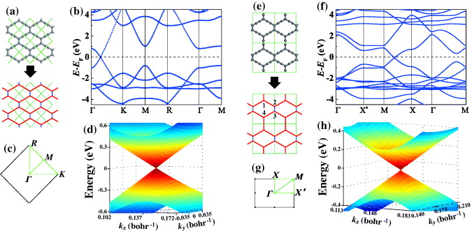
Figure 4. Prediction of Dirac cones in (a)–(d) 14,14,14-graphyne and (e)–(h) 14,14,18-graphyne. The atomic structure, band structure, Brillouin zone and three-dimensional band structure near Dirac points are shown. Four vertex carbon atoms in (e) are labeled with numbers from 1 to 4.
Download figure:
Standard imageThe first of these is 14,14,14-graphyne, which has a rhombic lattice with two vertex atoms in a unit cell as shown in figure 4(a). Each vertex atom is connected to its three nearest neighbors via one direct hopping (td) and two indirect hoppings through an acetylenic linkage ( ). Consequently, it is equivalent to graphene that is subject to a uniaxial strain along the armchair direction [6]. According to the criterion in the smallest honeycomb unit cell [32], if the three hopping terms can form a triangle, Dirac cones should exist. For 14,14,14-graphyne considered here, the values of
  and td are close to those in β and γ graphynes (see table 1), so we have
  , satisfying the triangular criterion. Therefore, 14,14,14-graphyne is a semimetal with Dirac cones (but is not metallic as claimed previously [9]), which was verified by first-principles calculations in figures 4(b)–(d).
The second type is 14,14,18-graphyne, whose atomic structure is very similar to 14,14,14-graphyne, but with the difference being that one direct hopping in the unit cell is replaced by an acetylenic linkage (see figure 4(e)). This graphyne has rectangular symmetry. Unlike the case of 14,14,14-graphyne, the rectangular unit cell of 14,14,18-graphyne with its four vertex atoms cannot be reduced into a smaller unit (i.e. one with two vertex atoms). First-principles calculations on the band structure indicate that 14,14,18-graphyne also possesses Dirac cones (figure 4(f)). In the vicinity of Dirac cones (±0.3 eV from the Fermi level), the valence and conduction bands exhibit linear dispersion in both the kx and ky directions with different slopes, namely 5.0 and 4.1 eV Å, respectively. The anisotropy of Dirac cones is related to the rectangular symmetry, just as with 6,6,12-graphyne [10]. Since 14,14,18-graphyne contains only four vertex atoms in a unit cell, the analyses become much easier. We performed an analytic study (see appendix B) and obtained an expression for the location of Dirac cones and the Fermi velocity, which confirms that Dirac cones locate at the X–M lines and that the Fermi velocity is direction dependent.
4. Conclusion
We have theoretically investigated the origin of the existence of Dirac cones in graphynes. We have constructed MLWFs from first-principles calculations and used the downfolding method to establish an effective TB model for graphynes. It was shown that the acetylenic linkages can be reduced into an effective hopping term, leading to the conclusion that all graphynes are topologically equivalent to graphene, and we clarified that different combinations of hopping terms give rise to the existence or absence of Dirac cones. The theory proposed here not only offers an explanation for the behaviors of Dirac cones in previous studies, but also is successful in predicting the existence of Dirac cones in two new graphyne systems, one of which has a rectangular symmetry.
Acknowledgments
We thank Jinying Wang and Honghao Li for valuable discussions. Support for this research was provided by the National Natural Science Foundation of China under grants numbers 2011CB921901 and 2011CB606405 and the Ministry of Science and Technology of China under grants number 11074139 to WD.
Appendix A.: Criterion for the existence of Dirac cones in α, β and γ graphynes
α, β and γ graphynes can be described by a unified TB model in a  honeycomb supercell with two kinds of hopping terms, tr and tb (represented by red and blue lines in figure 2(d)). The systems are bipartite with two interpenetrating sublattices, so the band structures are symmetric about the Fermi level under a TB approximation, and the criterion for the existence of Dirac cones is equivalent to that for the existence of discrete zero modes. We denote by x1, x2, ..., x6 the wavefunction values on the corresponding vertex carbon atoms. Then, the equations for the solution with E = 0 are given as
where k1 and k2 are the components of k on the reciprocal primitive vectors and L is the superlattice constant. {x1, x3, x5} are decoupled from {x2, x4, x6} due to the bipartite nature. Then the criterion for the existence of the solution becomes
which yields

It is determined from the imaginary part of (A.3) that k1 = 0 or k2 = 0 or k1 = −k2, i.e. the Dirac points are located at the Γ–M lines. Then we have eik1L + eik2L + e−ik1L−ik2L = 1 + 2 cos α (where α = k1L or k2L), whose value lies in the range of [ − 1, 3]. So the criterion becomes

whose solution is  and
and  .
.
Kim and Choi [14] have suggested a criterion for α, β and γ graphynes based on an analysis with a unit cell containing two vertex atoms. Their criterion is different from what we obtained here. The difference comes from the fact that β and γ graphynes should be described by a unit cell containing six vertex atoms as described here, but not two. This demonstrates the importance of hopping pattern in determining the existence/absence of Dirac cones in graphynes.
Appendix B.: Criterion for Dirac cones in 14,14,18-graphyne
14,14,18-graphynes can be described by a TB model in a rectangular supercell with two kinds of hopping terms,  and td. We denote by x1, x2, x3, x4 the wavefunction value on the corresponding vertex carbon atoms (figure 4(e)). Assuming the on-site energy is zero, the equations for the solution with any E are given as
where kx and ky are the components of k and Lx and Ly are the superlattice constants. Then the criterion for the existence of the solution becomes
which yields

Therefore, the criterion for the existence of Dirac cones corresponds to that of E = 0:

which can be rewritten as

So ky = 0 or kyLy = π, and the criterion is

When td and  have different signs, Dirac cones locate at ky = π and
  . When td and
  have the same sign, Dirac cones locate at ky = 0 and
  . The dispersion in the vicinity of Dirac points can be evaluated from (B.3), which gives direction-dependent Fermi velocity as
When the influence of the on-site energy is considered, Dirac cones still exist (details are not shown).