


Abstract
We systematically study the presence of narrow spectral features in a wide variety of random laser samples. Less gain or stronger scattering are shown to lead to a crossover from spiky to smooth spectra. A decomposition of random laser spectra into a set of Lorentzians provides unprecedented detail in the analysis of random laser spectra. We suggest an interpretation in terms of mode competition that enables an understanding of the observed experimental trends. In this interpretation, smooth random laser spectra are a consequence of competing modes for which the loss and gain are proportional. Spectral spikes are associated with modes that are uncoupled from the mode competition in the bulk of the sample.
Export citation and abstract BibTeX RIS

Content from this work may be used under the terms of the Creative Commons Attribution-NonCommercial-ShareAlike 3.0 licence. Any further distribution of this work must maintain attribution to the author(s) and the title of the work, journal citation and DOI.
1. Introduction
In random lasers, the combination of feedback by multiple scattering and gain leads to lasing [1–3]. Spectrally narrow emission features (typical line width of features <1 nm) have been found in a subset of the experiments on random lasers [4–6], whereas in other experiments the emission is narrowed but smooth (typical line width ∼3 nm) [2, 7]. The origin of the narrow spectral features, so called 'spikes', remains much debated in the multiple scattering community. From a laser physics perspective the appearance of a smooth emission spectra is just as peculiar. Understanding the crossover from smooth to 'spiky' spectra thus promises to give more insight into both random lasers and multiple scattering of light in general [3].
Historically, experimental groups have been divided between two schools of thought attributing spikes to either localized [4] or extended modes [6, 8]. More recently, three pioneering experiments have led to alternative explanations for the observation of spikes in random lasers. Fallert et al [9] argue that localized and extended modes can co-exist while reaffirming that strong scattering of light is a prerequisite for random lasing. Tulek et al [10] attribute lasing to resonators inside the sample [11] and argue that strong scattering is detrimental to random lasing. In the work of Leonetti et al [12] the explanation in terms of extended and localized modes is abandoned all together. The authors suggest that increasing coupling between modes is decisive in changing a random laser with a 'spiky' emission spectrum into a random laser with a smooth emission spectrum. Increased coupling can indeed lead to a merger of all resonances into one single spike. The line width of such a coupled system resonance is comparable to the line widths of uncoupled resonances. A coupling model alone can therefore only partly explain the transition from emission spectra with narrow spectral features to emission spectra with a single broad and smooth peak. Parallel to the ongoing experimental research, great progress has also been made in understanding random lasers theoretically. Several groups have shown that even the low-quality modes of a weakly scattering sample can end up as lasing modes in lower dimensional systems [13–15]. Despite these numerous studies in both theory and experiment, it remains a challenge to link insights in theory to experiment and vice versa.
Puzzled by the rich variety of interpretations in the random lasing community, we decided to investigate systematically how the gain length ℓg and the mean free path ℓ affect the occurrence of spikes in random lasers. We conjecture that the mean free path and gain length are the decisive quantities in understanding the physics of a random laser, because together they represent the two essential ingredients of any laser: feedback and gain. For this purpose, we have fabricated random laser samples over a wide range of gain and scattering strengths. While all other properties like material type, pump area and pump energy were kept fixed.
Statistical information on the properties of the narrow spectral features is important for the connection between new theories and experimental observations. However, only a small number of articles present such an analysis [10, 16, 17–22]. We characterize our random laser spectra by fitting every spike to a Lorentzian. These fitted functions provide us with a rich data set on the distribution of the spectral position and spectral spacing of spikes. Using a two-mode model that includes gain competition we are able to explain our results qualitatively.
2. Experimental methods
The studied random laser system is a dye solution (Rhodamine 640 P in methanol) in which elastically scattering titania particles (Ti-Pure R-900, DuPont) are dispersed. The characteristic interaction length scales are calculated using ℓ = 1/ρσ. In this formula, ℓ is the gain length (mean free path), ρ is the concentration of particles and σ is the stimulated emission cross section (scattering cross section). The stimulated emission cross section of the dye is 4 ± 0.5 × 10⁻²⁰ m2 at λ = 600 nm [7], and the scattering cross section of the colloids is ∼7 × 10⁻¹³ m2. The gain lengths reported in this paper assume all dye molecules are excited to the upper laser level and are therefore minimal values. In reality the gain length will be spatially dependent and longer than these reported gain lengths.
In our experiment, we aim to find a transition from spiky to smooth spectra in the ℓ–ℓg plane by applying a bisectional algorithm with respect to the scattering strength of our samples. At a fixed dye concentration, we start with a weakly and a strongly scattering sample. A new sample is then prepared after measuring these two samples. The scattering strength of the new sample is chosen such that it lies halfway in between those of the two closest measured samples that show opposite spiking behavior. This way, we minimize the difference between the scattering strength of our sample and the scattering strength for which the transition from smooth to spiky spectra occurs.
The bisectional algorithm is applied on systems having calculated minimal gain lengths of 4, 8, 16, 24, 32 and 40 μm (dye concentrations ranging from 10 to 1 mM). A small amount (0.1 g per 10 ml) of polyvinylpyrrolidone (PVP K-30) was added to the samples to ensure dispersive stability over several hours.
Samples are pumped with light at a wavelength of 535 nm, using 5 ns long pulses at a repetition rate of 20 Hz (Opolette). Emitted light is collected by the same lens that is used to focus the pump light on the sample. All experiments are conducted above threshold, with a pump power of 1.5 mW. The area of the slightly elliptical pump spot is 6.8 ± 1.4 × 103 μm2. For every sample, 100 single shot spectra are recorded using a spectrometer that is operated at a spectral resolution of either 1 nm or 0.1 ± 0.05 nm.
3. Data analysis and spike detection
The measured spectra are either smooth narrowed curves with respect to the below threshold spectrum or narrowed curves with distinct spikes superimposed on them. We have fitted all these individual spectra with Lorentzian lineshapes. After smoothing the data to remove noise, the number and position of spikes is found by analyzing the second derivative of the data. The locations of minima in the second derivative correspond to spikes in the spectrum. Only minima that are considerably deviating (10% of the difference between the global extrema) from their nearest maxima (larger than 0.1% of the original, smoothed data) are selected as corresponding to spikes. Using this method, we find the width, amplitude and position of every function representing either a spike or the narrowed background.
Figure 1 shows an example of a decomposed emission spectrum. The deviation of the original data to the fit is within 5% for the majority of the spectrum. This level of accuracy is typical for all spectra that have been analyzed. From this analysis, we conclude the fitting routine is able to reliably fit the elements of spiky spectra.

Figure 1. (Upper panel) Example of a fitted high-resolution spectrum. The black line is the original data, the blue curves are the individual components used to fit the data and the red curve is the fitted sum of all components. The fit parameters, height (I0), width (γ) and position (x0) are shown. (Lower panel) Residuals between the fit and the data. The gray area indicates a 5% deviation.
Download figure:
Standard image4. Results
4.1. Phase diagram: separating smooth spectra from spiky spectra
To study whether or not samples exhibit spikes, we analyze the average number of detected peaks. The inset in figure 2 shows the number of detected peaks per sample. A clear distinction can be made that separates spiky from smooth spectra as indicated by the dashed line. Sometimes more than one peak is detected in samples that on average are considered to be smooth. These deviations are due to unavoidable uncertainties in the fitting routine. Therefore, we only consider samples that on average have two or more detected peaks per spectrum as 'spiky' samples.
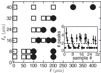
Figure 2. The appearance of spikes is shown as a function of the mean free path (ℓ) and gain length (ℓg) of each sample, measured at 1 nm resolution. Filled discs (•): samples with spikes. Open squares (□): samples without spikes. Spectra showing more than two distinct peaks are considered to contain spikes. The inset shows the average number of fitted functions per spectrum, the error bars represent the standard deviation.
Download figure:
Standard imageIn figure 2, the appearance of spikes is shown as a function of the sample parameters ℓ and ℓg. A clear trend is observed in this graph: spikes appear only in samples on the right-hand side of the diagram. This result already implies that strong multiple scattering is not a critical necessity for inducing spikes. In contrast, the more diffusive the sample becomes, the less likely it is that spikes will appear in the output spectrum. We note that both an increase in the transport mean free path and a decrease in gain length lead to a less diffusive sample (ℓ ≈ L with L being the system length), because a decrease in gain length makes a sample more absorbing and therefore leads to a shorter system length.
4.2. Spectral position of spikes
The obtained values for the fitting parameters allow us to study the statistics of spikes in much more detail. We use the high-resolution data to make sure all spikes are well separated.
Firstly, we analyze the spectral position of spikes and the broader background on which they reside. In figure 3(a), we show the spectral position distribution of both the fitted spikes (white bars) and the fitted broader background (gray bars) for one sample. The spectral spread for the position of the spikes is larger than the spectral spread for the position of the underlying spectrum. Moreover, the spikes reside predominantly on the blue side of the broad profile. The spectral positions are normally distributed. The distributions are fitted with Gaussians to enable comparison between different samples. In figure 3(b), the mean and variance of the spectral positions for the spikes are plotted versus the mean and variance of the underlying broad background. From this graph, we deduce that the emission wavelength of spikes is on average smaller than the central emission wavelength of the broad underlying profile for all samples.

Figure 3. (a) Distribution of the central emission wavelength of spikes (open bars) and broad background peaks (filled bars) for our model sample. Both distributions are fitted with Gaussian profiles (black curves). (b) The mean of the spectral distribution of spikes with respect to that of the corresponding background peak. The length of the error bars is determined by the width of the distributions; the spread in the position of the broad peak is much smaller than the spread in spike position. The dotted line indicates equality of the wavelengths.
Download figure:
Standard image4.3. Spectral spacing between spikes
Secondly, the spectral spacing between neighboring random laser spikes is retrieved from the fitted Lorentzian profiles. A typical distribution of spacing values for one sample is given in figure 4. The spectral spacing between the spikes is clearly peaked around 10 cm−1. We therefore deduce that level repulsion is present, a phenomenon previously reported for random lasers [19, 23]. We fit the spectral spacing distribution to Wigner's surmise with mean mode spacing (Δ) as the fit parameter. The fitted values for Δ are collected for several samples and are shown in the inset of figure 4. Surprisingly, we observe that the mean mode spacing is comparable for all systems that show spikes: Δ = 10.2 ± 0.9 cm−1. Since this analysis is performed for systems with different concentrations of scatterers and gain molecules, we conclude that the extent of level repulsion does not significantly depend on the strength of scattering or gain.

Figure 4. A distribution of spectral spacing values collected from one sample (bars). The curve represents Wigner's surmise fitted to the data. Inset: mean mode spacing as found by fitting Wigner's surmise to all collections of mode spacings. Samples with Δ = 0 cm−1 have smooth emission spectra.
Download figure:
Standard imageThe fitted values for Δ make it possible to compare our experimental results with theoretical random matrix calculations. Zaitsev [24] studied the mode spacing of a two-mode random laser theoretically. He concluded that for wide gain profiles, the spacing of the lasing modes does not depend on the spacing statistics of the passive system. His conclusion matches our experimental observation of a constant spacing for a wide range of sample parameters.
5. Two-mode model with gain competition
In order to build a basis for understanding the transition from smooth to spiky spectra, a model is set up consisting of just two laser modes. We stress that the presentation and discussion of this model are aimed at providing an intuitive understanding for the transition, but do not yet represent a rigorous theory. We first seek to answer how it is possible that emission spectra are smooth in a diffusive random laser. Then we consider several reasons for the occurrence of spikes in more weakly scattering media.
The quasi-modes in a diffusive sample have a wide range of decay times and overlap spatially on the intensity level. We therefore postulate that in a random laser, modes with different decay rates compete for the same gain. The number of photons in the two modes, q1 and q2, with cavity decay rates, γ1 and γ2, are described by two rate equations that both depend on the same number of molecules in the upper laser level N [25]:


Here we have considered a unit quantum efficiency gain medium with spontaneous emission decay rate Γ. The factors β1 and β2 describe which part of the spontaneous emission contributes to the lasing process and thereby determine the gain a mode receives. In a conventional laser, this β-factor is dependent on both the angular, βΩ, and spectral, βω, overlap between spontaneous emission and the mode [26]: β = βΩβω. We propose the solid angle normalized angular mode profile of the mode f(θ,ϕ) as a convenient way to determine the geometrical part of the β-factor by

One of the unique properties of a truly diffusive random laser is the fact that on average no angular mode selectivity takes place [7, 27]. Individual diffusive modes are speckle-like and, as a consequence, a single mode is omnidirectional as well. Given the speckle intensity Rayleigh distribution, all modes have a similar solid angle participation ratio, and therefore βΩ is constant for all modes. In the particular case of a random laser that has constant βΩ, the differences in the β-factor stem only from the spectral dependence of the β-factor. For the high gain modes with their spectrum centered around the peak of the gain curve, the β-factor then becomes proportional to the cavity decay rate. If we consider such a diffusive random laser by putting γ1/β1 = γ2/β2 = κ, we find from a steady-state analysis of equations (1)–(3): ![$q_1=q_2=\Gamma N/\left [\kappa - \Gamma N\right ]$](https://content.cld.iop.org/journals/1367-2630/14/11/113031/revision1/nj432847ieqn1.gif) . Surprisingly, two modes with a possibly widely varying decay time contain the same number of photons and have the same threshold. In layman's terms: modes that waste but also earn a lot become just as rich as frugal modes that earn very little.
. Surprisingly, two modes with a possibly widely varying decay time contain the same number of photons and have the same threshold. In layman's terms: modes that waste but also earn a lot become just as rich as frugal modes that earn very little.
In a three-dimensional diffusive random laser with a large excitation volume, the number of modes sharing the same gain medium is much larger than two. The number typically lies in the order of thousands [25, 28]. In addition, these diffusive modes are relatively lossy causing the spectral resonances to be spectrally broad and overlapping. If we extrapolate the aforementioned model to a system with many modes, we can conclude that in a diffusive random laser with a shared gain medium all modes close to the gain maximum end up with the same intensity. A superposition of these overlapping resonances with similar intensities then leads to the smooth output spectrum as observed in experiment.
To explain the observed spikes in random lasers we return to the simple model of two modes. Starting from a situation where γ1/β1 = γ2/β2 = κ, there are two ways to let one mode end up with more photons than the other mode. Firstly, by simply changing the ratio γi/βi (with i∈{1,2}) for the two modes. This ratio is decisive in determining which laser mode ends up with the majority of photons and thus profits the most from the available gain. The mode with the smallest ratio eats up the gain for the other mode, sometimes leading to a complete quenching of the second mode. Secondly, one mode can become more prominent when the gain competition is reduced by splitting up the gain in more than one reservoir. In this case, modes do not necessarily overlap and modes can occupy widely varying volumes. For a completely uncoupled system the number of photons in a lasing mode above threshold is given by R/γi + 1/βi, which shows that in such a situation the mode with the lowest cavity decay rate eventually becomes the most prominent in the spectrum.
To determine which of the two mechanisms is responsible for inducing spikes in our experiment, we have another look at the results shown in figure 3(b). For every cavity decay rate, there exists a spectral optimum where gain, absorption loss and cavity decay are balanced and subsequently the threshold is lowest. This optimum shift towards the red for slow cavity decay rates due to reabsorption losses [29]. At the blue side of the spectrum modes with fast cavity decay rates dominate over modes with slow cavity decay rates, which have a larger threshold. The fact that spikes appear systematically on the blue side of the spectrum, thus indicates that photons in the modes responsible for the spikes have traversed relatively short paths in the medium. The path length s is related to the cavity decay rate by si = c/γi. Apparently, and somewhat counterintuitively, spectral spikes represent modes with a large cavity decay rate. In a typical spectrum, several spikes appear simultaneously at the blue side of the spectrum, while a broader smooth peak remains present at the red side. From this observation, we conclude that mode competition cannot be ignored for modes with low cavity decay rates, while at the same time mode competition starts to play a less dominant role for the high cavity decay rate modes.
Our experimental phase diagram shows that spectral spikes appear when the sample becomes less diffusive. Once a random laser becomes less diffusive, that is ℓ ≈ L with L being the system length, βΩ ceases to be constant and modes are not by definition spread out over the whole sample. It is therefore likely that a compact mode with a short cavity decay time is privileged over long cavity decay modes. The confinement of this mode allows it to escape from the mode competition present amongst the other modes, enhancing its output. Multiple spikes can then appear in the spectrum representing other well confined modes. However, the more extended modes with low cavity decay rates are still competing for the same gain in the bulk of the sample, which leads to a broader but smooth peak in the spectrum. Reports in the literature on the spatial structure of random laser modes [9, 16, 19] showing that the extent of the modes associated with spikes are small compared to the excitation region, also support our interpretation that the narrow spectral features are due to confined modes with a high βΩ. A reduction of the system volume also facilitates the observation of narrow spectral features as observed in several experimental studies [9, 16]. Firstly, due to a decrease in the number of available modes and secondly, due to the fact that the system becomes less diffusive.
6. Discussion and conclusion
Our experimental observation of spikes being restricted to weakly scattering systems unambiguously shows that multiple scattering of light prevents the appearance of spikes. The results imply that spikes are caused by a process including only a low number of scattering events. We introduce a phase diagram that confirms previous indications of the importance of the ratio between the gain length and the mean free path in the literature [10, 30–32]. The statistics of the narrow spectral features is still largely uncharted territory. Our work reveals how rich the physics of random lasers becomes when studied systematically. We believe these statistical analyses are key for creating more satisfying connections between theory and experiment in the future.
The analysis of a simple two-mode model is able to explain the trends of our experiments qualitatively. The combination of a shared gain medium and the absence of angular mode selectivity in a purely diffusive random laser, leads to the simultaneous lasing of those modes close to the gain maximum. This simultaneous lasing in its turn creates a smooth output spectrum. Increasing either the gain or decreasing the transport mean free path moves the system away from the diffusive regime and thereby destroys the assumption of no angular mode selectivity and a completely shared gain medium. Individual modes become visible in the output spectrum that are characterized by short cavity decay times.
Our interpretation of random lasing in terms of mode competition also explains the results of some beautiful recent experiments [12]. Selectively feeding the modes in a random medium from the outside, as done e.g. in [12] by a non-isotropic excitation scheme, allows some modes to escape from the competition for gain inside the sample and to start lasing independently from the other modes. Our model, in which two modes are entirely dependent on the same gain reservoir, is undoubtedly an oversimplification of a random laser. In a typical random laser, thousands of modes are present with various spatial extents. We have implicitly made the assumption that such a system can effectively be studied by having one gain reservoir. Studying the break down of this assumption will surely lead to new and interesting insights into random lasers.
Acknowledgments
We thank Patrick Johnson, Claudio Conti and Sanli Faez for stimulating and helpful discussions. Daryl Beggs is thanked for a careful reading of the manuscript. This work is part of the research program of the 'Stichting voor Fundamenteel Onderzoek der Materie (FOM)', which is financially supported by the 'Nederlandse Organisatie voor Wetenschappelijk Onderzoek (NWO)'.