

Abstract
Understanding the phase diagram is the first step to identifying the structure–performance relationship of a material at the nanoscale. In this work, a modified nanothermodynamical model has been developed to predict the phase diagrams of Ag–Co nanoalloys with the size of 1 ∼ 100 nm, which also overcomes the difference in the predicted results between theory and simulation for the first time. Based on this modified model, the phase diagrams of Ag–Co nanoalloys with various polyhedral morphologies (tetrahedron, cube, octahedron, decahedron, dodecahedron, rhombic dodecahedron, truncated octahedron, cuboctahedron, and icosahedron) have been predicted, showing good agreement with molecular dynamics simulations at the nanoscale of 1 ∼ 4 nm. In addition, the surface segregation of Ag–Co nanoalloys has been predicted with a Co-rich core/Ag-rich surface, which is also consistent with the simulation results. Our results highlight a useful roadmap for bridging the difference between theory and simulation in the prediction of the phase diagram at the nanoscale, which will help both theorists and experimentalists.
Export citation and abstract BibTeX RIS
1. Introduction
In recent years, bimetallic clusters (also 'nanoalloys') have attracted much attention due to their peculiar properties and potential applications, which include magnetism [1, 2], optics [3, 4], nanosensors [5], and nanocatalysts [6, 7]. In particular, a large number of works have been focused on Ag–Co nanoalloys for catalysis [8]. For example, Holewinski et al found that the activity for the oxygen reduction reaction (ORR) of Ag–Co nanoalloys is five times higher than that of pure Ag catalysts, which also reaches over half the area-specific activity of the commercial Pt catalysts [9]. In addition, Ag–Co nanoalloys show higher catalytic activity for CO oxidation compared with pure Ag clusters [10]. Although Ag–Co systems at the nanoscale have been extensively studied [11], the phase diagram of Ag–Co nanoalloys remains largely unexplored. The main goal of this study is to fill this gap, and we predict the entire phase diagram of Ag–Co nanoalloys with various polyhedral morphologies (tetrahedron, cube, octahedron, decahedron, dodecahedron, rhombic dodecahedron, truncated octahedron, cuboctahedron, and icosahedron).
Because of the limitations of the experimental methods, the theoretical model and molecular simulation have become the commonly used methods for the prediction of phase diagrams [12, 13]. For example, many researchers have used the theoretical model such as Pawlow's law [14] as a simple way of predicting the melting temperature of clusters. It is found that the theoretical models were more convenient to predict the melting temperature of nanoalloys with the size of above 4–5 nm due to the consideration of the computational cost of molecular simulation [15]. Unfortunately, these theoretical models are still at an early stage, because they are based on a database of bulk materials and no clear method has yet emerged that can correctly interpret the variation of surface energy which varies with size in the small nano-system due to the nanometer size effect [16, 17]. In contrast, previous studies proved that molecular dynamics (MD) simulations are more efficient to accurately obtain the melting temperature of the nanoalloys compared to the theoretical prediction [18]. However, there is a difference between nanothermodynamical model-based theory and MD simulation in the prediction of melting temperature of nanoalloys [15]. To overcome the difference between theory and simulation, a new theoretical model needs to be developed.
In the present work, we develop a modified nanothermodynamical model to overcome the difference in the predicted phase diagrams between theory and simulation. Based on this modified model, we predict the phase diagrams of Ag–Co nanoalloys with various polyhedral morphologies with the size of 1 ∼ 100 nm. The predicted melting and surface segregation properties of these nanoalloys, using this model, are in excellent agreement with molecular simulations at the nanoscale of 1 ∼ 4 nm.
2. Computational details
2.1. The previous nanothermodynamical model
Since Takagi first reported the size-dependent melting temperature of small particles by means of a transmission electron microscope [19], a lot of models [20, 21] have been constructed to account for the dependence of melting temperature on particle size. As mentioned above, it has been shown that the previous nanothermodynamical model is only suitable for predicting the melting temperature of nanoparticles with the size above 4 nm, because the edge and corner of nanoalloy structures begin to make a significant difference on the melting properties with the size below 4 nm [22]. According to the previous nanothermodynamical model, the melting temperature,  for free-standing nanostructures can be expressed as a function of their corresponding bulk melting temperature,
  the size of the structure,
  and one shape parameter,
  The basic material properties of Ag and Co used in this work are listed in table 1. The size-dependent melting temperature,
  of a material at the nanoscale can be expressed as

where  is the melting temperature of a bulk material. The shape parameter,
  is defined as
  The numerical values of
  for different geometries (e.g. tetrahedron, cube, decahedron, etc) have been listed in table 2. D is the size of the structure (i.e. for a sphere, and D is the diameter).
  and
and  are the surface energy in the liquid and solid phases, respectively. A (m2) and V (m3) are the surface area and volume of the nanostructure, respectively.
Table 1. Basic material properties of silver and cobalt.
| Material properties | Ag | Co |
|---|---|---|
| Crystal structure [23, 24] | fcc | fcc |
| ΔHm·∞(kJ/mol) [23] | 11.297 | 16.20 |
| ΔHv·∞(kJ/mol) [23] | 250.6 | 376.6 |
| Tm·∞(K) [23] | 1234.93 | 1768 |
| γl(J/m2) [25] | 0.923 | 1.52 |
| γs(J/m2) [25] | 1.172 | 2.775 |
| atomic radius(Å) [26] | 1.44 | 1.25 |
Table 2. The correction parameters of α for different geometries.
| Morphologies | αAg | αCo |
|---|---|---|
| tetrahedron | 2.263 | 2.690 |
| octahedron | 1.434 | 2.029 |
| decahedron | 1.420 | 1.922 |
| dodecahedron | 0.511 | 0.921 |
| icosahedron | 0.751 | 1.252 |
| truncated octahedron | 0.557 | 0.978 |
| cuboctahedron | 1.308 | 1.352 |
| tetrahedron | 1.332 | 1.578 |
2.2. Monte Carlo simulations
Monte Carlo (MC) simulation is used to obtain the equilibrium structures of Ag–Co nanoalloys. This method is well documented in the previous work [27] and is found to be effective to obtain the equilibrium structures of bimetallic nanoalloys [28]. The interaction between metal atoms was modeled semi-empirically based on the well-established Gupta potential [29]. In the Gupta potential, the metal–metal (M–M) interaction energy,  is given by

where  and
and  are the Born–Mayer ion–ion repulsion and band interactions, respectively. These two terms for an atom
  can be represented based on


where  is the distance between atoms
  and
and  in the cluster.
  is the nearest-neighbor distance in the pure metals. The parameters


 and
and  for the pure species are fitted to the experimental values of the cohesive energy, lattice parameters, and independent elastic constants for the reference crystal structure at 0 K. The Gupta potential parameters for the Ag–Co clusters used in this study are taken from the literature [30] as listed in table 3, which were employed in previous studies with satisfactory results [31].
Table 3. Parameters of the Gupta potential for the Ag–Ag, Ag–Co and Co–Co interactions.
| A (eV) | ξ(eV) | p | q | r0(Å) | |
|---|---|---|---|---|---|
| Ag–Ag | 0.1043 | 1.1940 | 10.79 | 3.190 | 2.890 |
| Ag–Co | 0.1444 | 1.4776 | 10.01 | 3.085 | 2.695 |
| Co–Co | 0.1757 | 1.8430 | 9.21 | 2.795 | 2.500 |
2.3. Molecular dynamics simulations and thermodynamic parameters
MD simulations are performed using DLPOLY software [32] with a constant number of atoms N with a nearly zero fluctuating pressure P. The temperature was maintained by a Berendsen thermostat [33]. Newton's equations of motion were integrated using the verlet leapfrog algorithm and the integration time step was set to 1 fs. For the melting of the clusters, simulations were performed in a series of temperature conditions starting from 5 to 1300 K with a temperature increment of 50 K. The increment near the melting point was reduced to 10 K. At each temperature, the first 400 ps were used for the atomic structure equilibration, and the next 400 ps were used for the statistical averaging.
In this work, we identify the melting point of Ag–Co nanoalloys from the caloric curve of the Ag–Co nanoalloys and the corresponding heat capacity Cv per atom. According to the position of the maximum peak value in the heat capacity Cv and the step jump in the caloric curve, the melting temperature can be predicted. The heat capacity Cv per atom is defined by

where E is the potential energy,  is the Boltzmann constant, n is the total number of the atoms in the cluster and T is the temperature.
Here, we also employ the bond-order parameters (BOP) to further confirm the melting temperature of clusters. The BOP method was developed by Steinhardt et al to study supercooled liquids and metallic glasses [34]. The orientation of a bond r with respect to some reference system is specified by the spherical harmonics functions

where  and
and  are the polar and azimuthal angles of the bond r in this reference system. Global BOPs can be constructed by averaging over all bonds in the nanocluster:

where the sum runs over all Nb bonds in the system. In a similar way, the local BOPs for a given atom can be defined by averaging all bonds with its nearest neighbors. To avoid any dependence on the choice of the reference system, rotationally invariant combinations can be constructed as

where Ql and Wl are called the second-order and third-order invariants, respectively. Generally speaking, the BOPs Q4 are designed to identify structural transition during the melting process (Q4 ≈ 0.19 for face-centered-cubic structure and Q4 ≈ 0 for liquid structure). Therefore, the general idea of BOPs is to capture the symmetry of bond orientations regardless of the bond length so that the four BOPs have no unit.
3. Results and discussion
3.1. The modified theory
To calculate the phase diagram of a material at the nanoscale, the first step needs to evaluate the size-dependent melting properties of the material. In view of the previous thermodynamics model, the size-dependent melting temperature,  of a material at the nanoscale can be expressed as equation (1). As mentioned above, the previous nanothermodynamical model failed to predict the phase diagram of nanoalloys with the size below 4 nm [35, 36]. In contrast, the melting properties of nanoalloys with the size below 4 nm can be predicted by MD simulations. Figures 1(a) and (b) show the size-dependence of the melting temperature of Ag and Co clusters based on the previous nanothermodynamical model with the size of 4 ∼ 100 nm and MD simulations with the size of 1 ∼ 4 nm, respectively. It is found that a difference exists between the previous model and simulation in the prediction of the melting temperature of Ag and Co clusters.
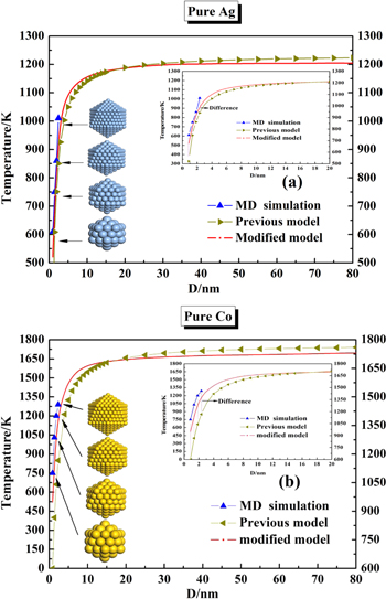
Figure 1. Size-dependence of melting temperature of icosahedral (a) Ag and (b) Co clusters based on the previous (4 ∼ 100 nm) and modified (1 ∼ 100 nm) nanothermodynamical model, and MD simulations (1 ∼ 4 nm).
Download figure:
Standard image High-resolution imageTo overcome the difference between the previous model and the MD simulations, a modified nanothermodynamical model was developed by introducing the correction parameters to account for the gap in the predicted results between theory and simulation as follows.

where  and
and  are the correction parameters used for the modified nanothermodynamical model. The aim of this modified model is to predict the size-dependent melting properties with the size of 1 ∼ 100 nm. Obviously, the development of the analytical expression for the correction parameters of
  and
and  is a crucial step for further application of the modified nanothermodynamical model in the prediction of the phase diagram.
In general, a quantitative understanding of the melting temperature of the nanoparticles can be obtained by considering the surface energy [15], metallic bond [37] and lattice parameters [38] while the latter two factors were not considered in the previous nanothermodynamical model. Thus, it is necessary to include the factors of the metallic bond and lattice parameters in the modified model. It is well known that both the metallic bond and lattice parameters are reflected in the cohesive energy. It is possible that the correction parameters of  and
and  in the modified nanothermodynamical model could be related to the cohesive energy. As mentioned in previous work [39], the mean cohesive energy per atom,
  and the cohesive energy of the bulk,
  can be calculated by the shape parameter, lattice parameter, and packing factor. The derivation was given as follows, and the number of surface atoms
  can be written as

where  is the atomic radius, which is deduced from the atomic volume
 and
and  are the radius of nanoparticle and shape factor, respectively.
  is the packing factor of the crystalline surface, defined as the ratio of the area of the plane occupied by atoms to the total area of the plane. For example, for an FCC lattice with a lattice parameter,
  we can calculate
  for (111) and (100) planes as
  and
and  .
.
Then, the volume of a nanoparticle, which is occupied by atoms, can be written as

where  is the volume of an atom,
  is the volume of the nanoparticle,
  is the number of interior atoms,
  is the number of surface atoms, and
  is the packing factor of the lattice.
  is defined as the ratio of the volume of the unit cell occupied by atoms to the total volume of the unit cell. Therefore, the cohesive energy of the nanoparticles
  is equal to
where  is the coordination number in the surface and
  is that in the lattice,
  is the energy of each bond. We know that
  so we introduce a parameter
  such that
  with 0 < q < 1.
So from equation (13),  is
is

For a large particle, tending towards the bulk, the number of surface atoms is negligible compared to that of the interior atoms, so  Therefore, the cohesive energy of the bulk material
  is given by
Therefore, from equations (11), (12), (14) and (15), we can have

where  is defined as the ratio of the volume of the unit cell occupied by atoms to the total volume of the unit cell.
  is the packing factor of the crystalline surface, defined as the ratio of the area of the plane occupied by atoms to the total area of the plane.
  is a constant,
  is the shape factor,
  is the atomic radius, and
  is the critical diameter.
In order to obtain the analytical expression of the correction parameters of  and
and  with the cohesive energy of
  and
and  we first fit
  and
and  based on the previous nanothermodynamical model with the size of 4 ∼ 100 nm and the results by MD simulations with the size of 1 ∼ 4 nm. A Matlab curve fitting tool (CFtool) is used for fitting
  and
and  Figures 1(a) and (b) show the size-dependence of the melting temperature of the Ag and Co clusters based on the modified nanothermodynamical model (1 ∼ 100 nm), respectively. It is found that the melting temperature obtained by the modified model shows good agreement with the MD simulations at the nanoscale of 1 ∼ 4 nm. Compared with the fitted correction parameters of
  and
and  and the cohesive energy of
  and
and  obtained by equation (16), the analytical expression of the correction parameters of
  and
and  can be written as

where  and
and  are the correction parameters used in this work.
  and
and  are the cohesive energies of the nanoparticle and bulk material, respectively.
  is the packing factor of the lattice.
  is the packing factor of the crystalline surface.
  and
and  are the atomic radius and the critical diameter, respectively.
  is the shape factor, and
  is a constant defined as
 is the coordination number in the surface and
  is that in the lattice. The correction parameters of
  and
and  obtained by the modified model for the Ag–Co systems with various polyhedral morphologies (tetrahedron, cube, octahedron, decahedron, dodecahedron, rhombic dodecahedron, truncated octahedron, cuboctahedron, and icosahedron) are summarized in table 4.
Table 4. The correction parameters of δ and λ obtained by the modified model for the Ag–Co systems with various polyhedral morphologies (tetrahedron, cube, octahedron, decahedron, dodecahedron, rhombic dodecahedron, truncated octahedron, cuboctahedron, and icosahedron).
| Morphologies | δAg | δCo | λAg | λAg |
|---|---|---|---|---|
| tetrahedron | 0.0157 | 0.0137 | 0.3496 | 0.5989 |
| octahedron | 0.0125 | 0.0109 | 0.4308 | 0.5284 |
| decahedron | 0.0123 | 0.0107 | 0.4347 | 0.5250 |
| dodecahedron | 0.0121 | 0.0103 | 0.4388 | 0.5212 |
| icosahedron | 0.0116 | 0.0101 | 0.4518 | 0.5102 |
| truncated octahedron | 0.0119 | 0.0102 | 0.4459 | 0.5178 |
| cuboctahedron | 0.0120 | 0.0104 | 0.4426 | 0.5182 |
| rhombic dodecahedron | 0.0122 | 0.0106 | 0.4387 | 0.5216 |
| cube | 0.0131 | 0.0114 | 0.4151 | 0.5421 |
3.2. Phase diagram
As mentioned above, the size-dependent melting properties of the material is the first step to calculate the phase diagram of a material at the nanoscale. As shown in figures 2(a) and (b), we calculate the size-dependent melting properties of pure Ag and Co based on equation (10). It is found that the melting temperature increases quickly with the size below 10 nm and then the melting temperature increases slowly and tends to stabilize with the size above 10 nm, which means the smaller nanometer size is more efficient in decreasing the melting temperature of nanoalloys with the size below 10 nm. And then, the set of size-dependent parameters  for any sizes selected (here, 2, 4, 6, and 10 nm) can also be obtained by equation (19).


Figure 2. Size-dependence of the melting temperature of (a) pure Ag and (b) pure Co clusters based on the modified nanothermodynamical model.
Download figure:
Standard image High-resolution imageIn this work, Ag and Co share the same crystal structure at the nanoscale (fcc crystal-structured Ag and Co is considered) [23, 40] and similar atomic radii (less than 14%) [26]. Therefore, according to the Hume–Rothery's rules [41], we calculate the phase diagram at the bulk, as shown in figure 3 (black field). In addition, the solidus−liquidus curves of the Ag–Co alloys are given by
where  and
and  are the melting enthalpies of the bulk materials of A and B, respectively.
  is the composition in the solid (liquid) phase at a given
 and
and  are the bulk melting temperatures of Ag (A) and Co (B), respectively.
  is the characteristic ideal gas constant. Martienssen et al have clarified most of the materials data in the Springer Handbook including the value of
  and
and  for Ag and Co, as listed in table 1. And then, based on the size-dependent parameters
  calculated above, the liquidus and solidus curves [42] can be calculated from equation (21) as follows and then the Ag–Co phase diagrams at the nanoscale can be produced.
where  and
and  are the melting enthalpies of materials at the nanoscale and bulk, respectively.
  is the composition in the solid (liquid) phase at a given
 and
and  are the size-dependent melting temperatures of Ag (A) and Co (B), respectively.
  and
and  are the size-dependent melting enthalpies of Ag (A) and Co (B), respectively.
  is the characteristic ideal gas constant.

Figure 3. Phase diagrams of the Ag–Co systems at the bulk scale (black) and at 2 (magenta), 4 (blue), 6 (green), and 10 nm (orange) for (a) tetrahedron, (b) octahedron, (c) decahedron, (d) dodecahderon, (e) icosahedron, (f) truncated octahedron, (g) cuboctahedron, (h) rhombic dodecahedron, and (i) cube. The black arrow is used to highlight the size effect on the melting point.
Download figure:
Standard image High-resolution imageThe phase diagrams of Ag–Co nanoalloys with various polyhedral morphologies (tetrahedron, cube, octahedron, decahedron, dodecahedron, rhombic dodecahedron, truncated octahedron, cuboctahedron, and icosahedron) [43, 44] are plotted in figure 3. In particular, as shown in figure 3, we predict the phase diagram of Ag–Co nanoalloys below 4 nm based on the modified nanothermodynamical model for the first time. The melting temperatures of nanoalloys are found to be significantly lower than those of the bulk material, which is in agreement with experimental results [38] and previous theoretical considerations [45, 46]. Moreover, with increasing the size, the lens width decreases and the phase diagram at the nanoscale is close to that at the bulk. In the lens-shape region, this is a two-phase field where the liquid is at equilibrium with the solid phase, above and below where the solution is purely liquid or solid. In addition, these nanoalloys with the morphologies of dodecahedron, truncated octahedron and icosahedron exhibit high solidus curves, which are similar to the previous studies [15, 47]. It may be attributed to the geometrical considerations [48], such as the A/V ratio and the number and type of facets.
3.3. Melting temperature prediction
Based on the phase diagram, we can define the solid–liquid transition temperature as the melting temperature, so that we can further predict the melting temperature of Ag–Co nanoalloys with the size of 1 ∼ 100 nm. To compare the melting temperature with MD, we performed a set of MD simulations before predicting the melting temperature by phase diagram. Figure 4(a) shows the caloric curve and the heat capacity Cv of icosahedral Ag–Co nanoalloys with the ratio of Ag–Co (1:1) and different sizes of 55, 147, 309 and 561, respectively. Figure 4(b) shows the temperature dependence of BOPs Q4 for Ag–Co nanoalloys. It is found that a great jump in the Q4 values appears at higher temperature due to the atomic vibrations upon melting, which corresponds to the occurrence of the melting and is in good agreement with the position of the maximum peak value in the heat capacity Cv and the step jump in the caloric curve (see figure 4(a)). At the temperatures after melting, Q4 ≈ 0 is found, corresponding to the appearance of the liquid phase. The details of identifying the melting temperature and definition of thermodynamic parameters in MD can be found in section 2 and previous works [49, 50].

Figure 4. Temperature dependence of the caloric curve and  curve for the Ag–Co (1:1) nanoalloys with different sizes of 55, 147, 309 and 561(a) and BOP parameter Q4 for Ag–Co nanoalloys (b).
Download figure:
Standard image High-resolution imageAnd then, we further predict the melting temperature by phase diagram based on the modified model. Figure 5(a) shows the melting temperature of icosahedral structured Ag–Co nanoalloys predicted by the modified nanothermodynamical model and MD simulation. Moreover, the melting temperatures predicted by the previous model are added in figure 5(a). Compared to the melting temperatures predicted by the previous model, it is found that the melting temperature predicted by the modified model is in excellent agreement with the melting temperatures predicted by MD simulation, which confirms that the modified model is more efficient than the previous model. In addition, the melting temperature of octahedral structured Ag–Co nanoalloys is predicted by the modified model and MD simulations as shown in figure 5(b), which also shows the high-efficiency of the modified model in predicting the melting temperatures. The melting temperatures of Ag–Co nanoalloys with different morphologies and a fixed composition of Ag50Co50 are also predicted by the modified model, as shown in figure 5(c). From figure 5(c), we can find the same variation trend for the melting temperature, which varies with size for different types of nanoalloys, so it is evident that size plays an important role on the thermal stability of nanoalloys. This phenomenon has already been found in many other nanoalloys [14, 51].
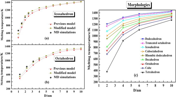
Figure 5. Melting temperature of Ag–Co nanoalloys versus size for icosahedron (a) and octahedron (b) predicted by the previous model, the modified model and MD simulations, and (c) for all the investigated morphologies with the fixed composition of Ag50Co50.
Download figure:
Standard image High-resolution image3.4. Surface segregation prediction
Structurally, the surface segregation of Ag–Co nanoalloys has also been predicted based on the phase diagram, which is in good agreement with the molecular simulation results. As is known, surface segregation leads to a new atomic species repartition between the core and the surface due to the composition difference. According to Williams and Nason [52], the surface composition of the liquid and solid phase are given by:
Here,  and
and  are the solidus and liquidus composition given by the set of equation (21), respectively.
  is the difference between the bulk vaporization enthalpies of the two pure elements,
 is the difference between the bulk sublimation enthalpies of the two pure elements,
 is the first nearest neighbor atoms, and
  is the number of first nearest atoms above the same plane (vertical direction). For example, in the case of the face-centered cubic (fcc) crystal structure of Ag and Co materials, we have
 for (100) faces and three for (111) faces.
  is the characteristic thermal energy. For icosahedral structured Ag−Co nanoalloys with a size edge length of 2 nm, we can see that the lens shape of the surface liquid/solid curves is deformed compared to the core, as shown in figure 6(a). At a given temperature, the liquid and solid curves of the surface are enriched in Ag compared to the core, which is in good agreement with the previous experimental [9] and simulation observations [30, 53]. In figure 6(b), we consider the surface segregation of Ag–Co nanoalloys with the octahedron and the size edge length of 4 nm. It is found that the surface segregation phenomena of Ag–Co nanoalloys with the morphology of an octahedron is similar to the segregation trend for icosahedral Ag–Co nanoalloys, indicating that the morphology and size effects can be ignored in the segregation phenomena of Ag–Co nanoalloys. In addition, MD simulations confirm the preferential presence of Ag at the surface and show good agreement with the results predicted by the phase diagrams at the same scale of 2 and 4 nm.
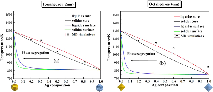
Figure 6. Phase diagram of Ag–Co nanoalloys considering the surface segregation effect (a) for an icosahedron with the size of 2 nm, and (b) for an octahedron with the size of 4 nm.
Download figure:
Standard image High-resolution imageAiming at further confirming the surface segregation phenomena of Ag–Co nanoalloys, we have performed a set of MC simulations to calculate the energy per atom and the excess energy of a Ag–Co nanoalloy. In this work, we considered two special types of nanoalloys due to the fact that icosahedral and octahedral nanoalloys are of high structural stability and have been commonly used in previous works [54, 55]. The excess energy,  was usually adopted to represent the relative stability of the clusters [56]. In this work, the excess energy
  of the Ag–Co cluster is defined by
where  is the total energy for a given cluster, and
  and
and  are the total energies for the pure
  and
and  clusters, and
  is the total number of the cluster. Clearly, the lower the value of
  the more stable the structure of the cluster. The results are summarized in table 5. It is found that the excess energies of the icosahedral and octahedral structured Co-core/Ag-shell nanoalloys are much smaller than those of the Ag-core/Co-shell nanoalloys. It means that the Ag-shell/Co-core structure is more stable than the Ag-core/Co-shell one, which is in good agreement with the surface segregation of Ag–Co nanoalloys with a Co-rich core/Ag-rich surface as predicted by the phase diagram (see figure 6).
Table 5. The energy per atom and excess energy of pure Ag, pure Co and Ag−Co nanoalloys (icosahedron: size edge length of 2 nm; octahedron: size edge length of 4 nm).
| Morphology of NAs | Snapshot | Structure | Component | Mean energy per atom (eV) | Excess energy Δ (eV) |
|---|---|---|---|---|---|
| Icosahedron |
 |
Pure Ag | 309 Ag | −2.743 | 0 |
| Icosahedron |
 |
Pure Co | 309 Co | −4.148 | 0 |
| Icosahedron |
 |
Co/Ag core/shell | 162 Ag 147 Co | −3.459 | −14.739 |
| Icosahedron |
 |
Ag/Co core/shell | 162 Co 147 Ag | −3.486 | −1.7922 |
| Octahedron |
 |
Pure Ag | 3281 Ag | −2.757 | 0 |
| Octahedron |
 |
Pure Co | 3281 Co | 3.979 | 0 |
| Octahedron |
 |
Co/Ag core/shell | 1028 Ag 2253 Co | 3.750 | −233.94 |
| Octahedron |
 |
Ag/Co core/shell | 1028 Co 2253 Ag | 3.158 | −58.40 |
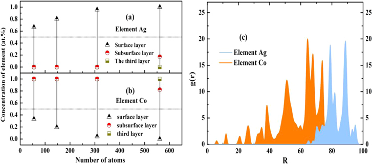
In order to understand the surface segregation phenomena of Ag–Co nanoalloys in more detail, the concentration of Ag and Co atoms in the surface, subsurface and third (from subsurface to center) layers for the icosahedral Ag–Co nanoalloys as a function of the different sizes of 55, 147, 309, and 561 are also plotted in figures 7(a) and (b), respectively. The results show that Ag concentration in the surface layer is around 16 ∼ 50 at.% higher than the overall Ag concentration in the Ag50Co50 nanoalloys. Accordingly, the Ag concentration in the subsurface and third layers is much lower than the overall Ag concentration in the Ag50Co50 nanoalloys. Figure 7(b) shows the concentration of Co in the surface, subsurface and third layers of the Ag50Co50 nanoalloys changing with the cluster size. In contrast to the increasing Ag concentration, the Co concentration in the surface layer decreases with the increasing of the size, which is around 18 ∼ 50 at.% lower than the overall Co concentration in the nanoalloys. The results further confirm that Ag atoms tend to locate at the surface sites of Ag–Co nanoalloys.
Figure 7. Calculated concentration of Ag (a) and Co (b) elements in the surface, subsurface and third (from surface to center) layers of the Ag–Co clusters with the composition of Ag50Co50 as a function of the cluster size at 300 K (Dotted line represents the overall Ag or Co concentration in the nanoalloys.). The pair of correlation functions of the Ag–Co nanoalloys (561 atoms) with the composition of Ag50Co50 at 300 K (c).
Download figure:
Standard image High-resolution image
The pair of correlation functions of the Ag–Co icosahedral nanoalloys (561 atoms) with the composition of Ag50Co50 at 300 K are also supplied in figure 7(c). The pair of correlation functions is given by

where N is the total number of the atoms in the cluster and  is the distance between atoms i and j,
  are the coordinates of the center of mass at each MC step. As shown in figure 7(c), the Ag atoms are enriched on the surface, and the Co atoms are mainly in the inner core. This observation is consistent with our calculated concentration of Ag and Co atoms in the surface, subsurface and third layers of the icosahedral Ag–Co nanoalloys, as shown in figures 7(a) and (b). A qualitative understanding of the predicted segregation phenomena of the Ag-rich atoms on the surface can be obtained by considering the thermodynamic reasons such as the surface energies [57], the bonding energies [30], and the lattice parameters [26].
4. Conclusions
In conclusion, a modified nanothermodynamical model has been developed to predict the phase diagrams of Ag–Co nanoalloys at the full scale of 1 ∼ 100 nm, which overcomes the significant difference in the predicted results between theory and simulation for the first time. Based on the modified model, the phase diagrams of Ag–Co nanoalloys with various polyhedral morphologies (tetrahedron, cube, octahedron, decahedron, dodecahedron, rhombic dodecahedron, truncated octahedron, cuboctahedron, and icosahedron) have been predicted, showing the consistency of the theoretical and simulation results at the same scale of 1 ∼ 4 nm. Moreover, the surface segregation of Ag–Co nanoalloys has also been predicted with a Co-rich core/Ag-rich surface, which is also in good agree with the simulation results. Our results highlight a useful roadmap for bridging the difference between theory and simulation in the prediction of a phase diagram, which will provide insight into the structural and thermal information for both theorists and experimentalists.
Acknowledgments
This work is supported by the National Natural Science Foundation of China (21576008, 91334203), the Beijing Higher Education Young Elite Teacher Project, the BUCT Fund for Disciplines Construction and Development (Project No. XK1501), Fundamental Research Funds for the Central Universities (Project No. buctrc201530), the 'Chemical Grid Project' of BUCT and the Supercomputing Center of the Chinese Academy of Sciences (SCCAS).