

Abstract
It could be argued that activity measurements of radioactive substances should be under statistical control, considering that the measurand is unambiguously defined, the radioactive decay processes are theoretically well understood and the measurement function can be derived from physical principles. However, comparisons invariably show a level of discrepancy among activity standardisation results that exceeds expectation from uncertainty evaluations. Also decay characteristics of radionuclides determined from different experiments show unexpected inconsistencies. Arguably, the problem lies mainly in incomplete uncertainty assessment. Of the various reasons leading to incomplete uncertainty assessment, from human failure to limitations to the state-of-the-art knowledge, a selection of cases is discussed in which imperfections in the modelling of the measurement process can lead to unexpectedly large underestimations of uncertainty.
Export citation and abstract BibTeX RIS

Original content from this work may be used under the terms of the Creative Commons Attribution 3.0 licence. Any further distribution of this work must maintain attribution to the author(s) and the title of the work, journal citation and DOI.
1. Introduction
'[...] as we know, there are known knowns; there are things we know we know. We also know there are known unknowns; that is to say we know there are some things we do not know. But there are also unknown unknowns – the ones we don't know we don't know.'
—Donald Rumsfeld
1.1. Known knowns
The measurand of an activity measurement is (the expectation value at a reference time of) the number of radioactive decays per second of a material, expressed in the SI derived unit becquerel (1 Bq is 1 aperiodic event per second). With each spontaneous disintegration of a nucleus, at least one type of radiation (photons and/or particles) is emitted and therefore decays can in principle be detected and counted [1]. Activity measurements benefit from a good theoretical understanding of the processes that occur [2]. Establishing the becquerel [3–5] for a suite of important radionuclides is made possible due to the high accuracy by which the measurement process can be modelled. Good metrology implies statistical control of the uncertainties. Random errors are typically reduced by repetitions to an extent that they contribute negligibly to the uncertainty budget. Realistic models allow establishment of propagation factors between the estimate of the measurand and all variables contributing to its uncertainty [6].
We know that nuclear decay is randomly distributed in time, that the activity of a radioactive source diminishes exponentially and that the half-life of the radionuclide determines the slope of the decay curve [7, 8]. We have built up a rich database of decay characteristics for thousands of radionuclides [9–13]. We know the different types of radiation emitted, have a good understanding of the interaction of radiation with matter, and by extension know which signals to expect in various detectors [2]. Computer simulations can reproduce particle and photon transport in complicated experimental designs [14–18]. Spectral interference of signals can be deconvoluted with heuristic peak shape models [19, 20]. Statistical aspects of nuclear counting have been explored in theory and practice, live-time techniques were developed to compensate for dead time and pileup [1, 21]. Established primary standardisation techniques have been described in literature [4, 22], as well as a detailed analysis of their relevant uncertainty components [23]. Already for decades, the same physical principles are being used for detection and the attainable accuracy on the activity per mass of a mononuclidic solution is of the order of 0.1%.
1.2. Known unknowns
In spite of the vast theoretical and metrological knowledge on radioactivity accrued over more than a century, there are limits to the detail in which decay characteristics can be modelled or predicted and to the completeness and accuracy of the thousands of decay schemes. Surprisingly, many decay characteristics of even the most relevant <100 nuclides [11] are still in need of improvement for optimal use in applications for nuclear energy, medicine, safety and security, environmental monitoring, nuclear dating, astrophysics, etc [24–30]. Many decay data were measured more than 50 years ago and new measurements offer advantages of advanced detection and data processing techniques, enhanced attention to uncertainty evaluation as well as harmonised and transparent reporting thereof using the concepts and terminology of the GUM [6].
Experienced metrologists are aware of the state of imperfection of radionuclide metrology [31]. The inconsistencies among measured decay data in literature are so significant that data evaluators invest much effort in analysing and comparing experimental data with the aim of deriving one recommended set of values in a coherent decay scheme [9–13]. Intercomparisons typically show signs of discrepancy among the activity measurements performed by routine laboratories [32] as well as the primary standardisations laboratories [33]. Whereas the uncertainties provided by the laboratories are informative in the sense that they are indicative of the deviations between the measurement results and the mean, they generally do not fully cover the variation of data. In spite of agreement on the uncertainty propagation rules set out in the GUM, there is no uniformity in the estimation of the size of the uncertainty components [34–36]. Also propagation of correlated data [37] is not always applied rigorously in practice.
To address these issues, experts from national metrology institutes (NMIs) have contributed to a special issue of Metrologia dealing with 'known unknowns' in radioactivity measurements [23], with a focus on primary standardisation methods and analytical techniques which are used to realise the SI unit becquerel. For each technique, an in-depth analysis is performed of the uncertainties coming into play, and where possible formulas and typical values are presented. This work is intended to serve as a consolidated foundation and a key resource for the handling of uncertainties in radioactivity measurements. It impacts ultimately every radioactivity measurement in the world through the use of SI-traceable calibration standards and fundamental decay data produced by reference laboratories.
1.3. Unknown unknowns
Unknown errors only reveal themselves as inconsistencies in comparison with other measurement results, possibly in the shape of unexpected variance in repeatability studies, discrepancies among various methods, laboratories, literature data, etc. Absence of such indicators makes us oblivious of hidden sources of error affecting the accuracy of the measurement. They may be tackled by an active search based on reason and completing the metrological puzzle using all possible hints, somewhat comparable to the discovery of dark mass and dark energy in cosmology [38]. Lack of investment into a deeper understanding of every aspect involved leads to overconfidence in the outcome as well as the interpretation of the measurement.
A pro-active view is more likely to be found in a 'bottom–up' approach of uncertainty evaluation, as advocated by the GUM, rather than a more passive 'top–down' philosophy. Take for example an observer having one clock. Without scrutiny into the technical details behind the working mechanisms of the clock, the observer may assume that the clock shows time with absolute precision. From a 'top–down' point of view, doubt only arises when additional clocks become available and an uncertainty value is assigned to cover the discrepancies among the time indications. Initially, the growing number of available clocks would seemingly increase the uncertainty on the average time. This contradiction should not occur if the uncertainty were adequately derived from in-depth technical scrutiny, thus providing insight in the errors that each clock may produce, as well as differences in accuracy that may be expected from each clock, and assignment of relative importance of each readout to obtain the best combined estimate.
Lack of knowledge of the intricacies behind a measurement should not necessarily be interpreted as an absolute gap in our collective understanding. Most aspects in radionuclide metrology have been studied in detail by various theoretical, experimental and metrological experts, and have been conveyed through literature and software at some point, but may have been overlooked or ignored in metrological practice. Experience is continuously lost and regained with new generations of scientists and metrologists taking over from the old. Metrology as an art demands sound theoretical knowledge about the measurand and its properties, as well as many years of continued investment to gain control over the methodology.
At times, the complexity of the interaction of a multitude of influencing parameters incites the metrologists to oversimplify the functional model describing the measurements, thus ignoring significant contributors to the uncertainty budget. Typical examples are: being unaware of inaccuracies in decay schemes of radionuclides, ignoring uncertainties on atomic and nuclear data used in computer simulations, and not controlling every aspect of the measurement device and the radioactive sample. Pieces of equipment and analytical software are often treated as 'black boxes' of which the output is accepted in good faith. The richness of an uncertainty budget is measured in its completeness, not so much in the smallness of the final number.
1.4. Incomplete models and failing interpretations
Of the various reasons leading to incomplete uncertainty assessment, from human failure to limitations to our state-of-the-art knowledge, in this paper a selection of cases will be discussed in which imperfections in the modelling of the measurement process can lead to unexpectedly large underestimations of the uncertainty in radionuclide metrology.
2. Canaries in the coal mine
2.1. Redundancy and comparison
First awareness of uncertainty comes to the metrologist when being unable to answer certain questions which may be relevant to the measurand and the methodology used to quantify it. Any unanswered question should give rise to an item in the uncertainty budget and an estimate should be made to quantify its potential impact on the result. Most metrologists will recognise the sobering moments in their lives when repeated measurement did not confirm previously obtained results within the expected precision. Having expanded their uncertainties accordingly, a new disappointment may arise from comparing with data obtained by an alternative technique. In particular with primary standardisation measurements, redundancy of techniques is an important asset to establish a reliable reference value, as there is no arbiter on the 'true value'.
In key comparisons of activity measurements, national metrology institutes provide a value for the activity per mass of a radionuclide in solution, all participants being provided one aliquot of the same material. Redundancy of measurement techniques sometimes reveals their strengths and weaknesses. For example, a liquid scintillation counting method (LSC C/N) [39] proved to be ideally suited for the activity standardisation of 204Tl, as it suffered less than other methods from self-absorption of the low-energy beta radiation in the source material [40]. On the other hand, the same method did not perform well in the standardisation of 125I, as could be demonstrated in comparison with a wide variety of alternative methods [41, 42]. Therefore, it would be short-sighted policy to reduce the amount of techniques used for reference measurements, since redundancy of methods is an absolute must to alert for systematic errors in a particular method for a particular measurand.
However, discrepancies also show up in absence of clear outliers or manifest systematic errors associated with a technique. Arguably, the problem lies mainly in the uncertainty assessment itself. In an intercomparison, national metrology institutes were given the same 4πβ − γ coincidence measurement data and asked to derive an activity and uncertainty by mathematical analysis. Whereas the activity values were quite consistent, the estimated uncertainty differed by a factor of 3, and even larger differences occurred in the relative size of the uncertainty components [34]. A similar exercise was done on the analysis of 99Tc data obtained by triple-to-double coincidence counting (TDCR). Interestingly, the participants obtained different results for the activity concentration and the largest estimated relative standard uncertainty was more than 7 times larger than the lowest value [35]. An intercomparison on emission rate measurements of beta and alpha particles from large area sources revealed that the dominant uncertainty contributions were treated in a non-uniform manner and laboratories had different approaches to identify and evaluate input quantities in the model function [36]. In this context, the GUM Supplement 1 [43] recommendation to simulate the shape of the probability density function is a non-issue as long as its width is so poorly known.
2.2. Meta-analysis
The way data are presented influences the perception thereof: in the particular case of intercomparison results, the importance of realistic uncertainty evaluation can be emphasised through 'degree of equivalence' (DoE) graphs as applied in the BIPM key comparison database (KCDB) [44] or by means of novel data representations, such as the PomPlot [32, 33]. In a DoE graph, equivalence of a laboratory result with the reference value is demonstrated when the expanded (k = 2) uncertainty bar of their mutual difference D = x − xref overlaps with zero. In the PomPlot, data are presented by a symbol in a (x, y) plot with D and the combined standard uncertainty u(D) on the axes (both normalised by the median absolute deviation or MAD). The level of equivalence is shown by zeta score lines (ζ = 1, 2, 3) creating a pyramid-like shape. PomPlots can be made of one intercomparison, a combination of comparisons or a targeted selection of data such as all comparison results of one particular laboratory.
In figure 1, a PomPlot is shown of key comparison results for activity standardisations of different radionuclides as published in the KCDB up to the year 2005 [33]. The graph gives an intuitive impression of the level of accuracy in radionuclide metrology. Whereas a majority of the data appear within the ζ = 3 lines, there are ample outliers demonstrating that the sources of uncertainty are not fully under statistical control. The correlation between the claimed uncertainty u and the deviation D of the result is not as strong as could be expected. PomPlots with results of individual laboratories seem to reveal recurrent trends with respect to the accuracy of their results and the comprehensiveness of their uncertainty budgets [32, 33].
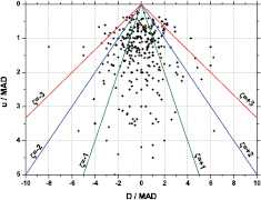
Figure 1. PomPlot combining the available key comparison results for activity standardisations of different radionuclides up to the year 2005 [33].
Download figure:
Standard image High-resolution imageFigure 2 shows histograms of the average values <|D|>, <|D|/u1/2>, <|D|/u> for selected regions of u/MAD. The mean deviations are positively correlated with the uncertainty, but not exactly proportional since the ratio |D|/u is negatively correlated with u. This is an indication of the rate by which uncertainties are underestimated (<|D|/u  1) and overestimated (<|D|/u> <1). Interestingly, there is a better proportionality of |D| with the square root of the uncertainty. This is also clear from the PomPlot in figure 3, in which the u/MAD was replaced by (u/MAD)1/2. The data are more concentrated around (u/MAD)1/2 = 1, yielding less outliers in the top region and less overestimated uncertainties in the bottom region.
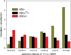
Figure 2. Measures of average deviation, <|D|>, <|D|/u>, <|D|/u1/2> as a function of U = u/MAD [33].
Download figure:
Standard image High-resolution image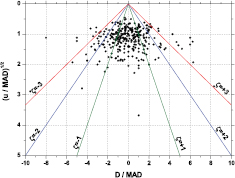
Figure 3. Hypothetical PomPlot of the available key comparison results, replacing the uncertainty by a square root value (see text) [33].
Download figure:
Standard image High-resolution imageThe fact that outliers are mainly situated at the top of the graph may partly be due to the omission of statistical weighting in the calculation of the reference values from arithmetic means. However, an inverse variance weighted mean (w ~ u−2) is overly attracted to data with underestimated uncertainty and inherently leads to underestimation of its uncertainty [45]. The evidence in figures 2 and 3 suggest that, for the KCDB data, a weighted mean using the standard deviations as weighing factor (w ~ u−1) should be less sensitive to bias caused by incorrect uncertainty assessments. The commonly raised argument that 'there is no mathematical basis' for weighting by w ~ u−1 overlooks the fact that u represents only a rough estimate of the standard uncertainty which can deviate from the real value by a factor of 3 in either direction (see section 2.1). Statistical theory does not rigorously apply, since it relates to another reality.
The calculation of a mean value and realistic uncertainty from a discrepant data set has been extensively studied (see references in [45]). The discrepancy problem is often presented as due to an unexplained inter-laboratory bias, whereas imperfect uncertainty assessments are the more plausible root cause. Based on the latter paradigm, an effective strategy has been implemented in the 'power-moderated mean' (PMM) [45]: the weighting is moderated by increasing the laboratory variances by a common amount and/or decreasing the power of the weighting factors. Computer simulations show that the PMM provides a better trade-off between efficiency and robustness for data with 'informative but imperfect' uncertainty estimates then some popular methods used in clinical studies. Since 2013, the PMM is the designated method to calculate the key comparison reference values within section II of the consultative committee for ionising radiation, CCRI(II).
3. Modelling of the detection process
3.1. Monte Carlo simulations and analytical models
Monte Carlo (MC) simulations are frequently used to model various aspects of the measurement process [46]. General purpose particle transfer codes [14–18] can reproduce physical processes in customer designed geometries, which has important applications such as the calculation of detection efficiency of a radioactive source in gamma spectrometers [47], ionisation chambers [48] and various other set-ups [49–52]. Additionally, detailed analytical models have been developed for specific applications, such as efficiency calculations in liquid scintillation counting [51], high-geometry 4πγ counters [52] and defined solid angle counters [53]. MC simulations are also used for non-trivial uncertainty propagation calculations as recommended in an annex of the GUM [43] and specific examples have been expanded on [54].
In general, the models are used to reproduce complex situations involving a multitude of influential parameters on the measurement conditions, incl. source-detector geometry, composition of intervening materials, transport of primary and secondary particles produced by decay and nuclear reactions and interactions with material. A high level of realism can be achieved with carefully designed simulations, but a full uncertainty budget on the simulated result requires insight in the dominant uncertainty components. There is no measurement function available from which sensitivity factors can be derived. Detailed studies of the influence of intervening parameters, e.g. in γ-ray spectrometry [55–58], are rare.
Analytical models may be less flexible and accurate than MC simulations, but they are better suited to investigate the sensitivity factors, because the calculations are faster and have perfect repeatability [52, 53]. Sensitivity factors can be derived from varying geometrical and nuclear parameters one by one in successive calculations. Simple analytical models can reveal dominant terms and their functional behaviour [52, 53]. MC simulations miss flexibility and statistical accuracy in this respect.
Although counting statistics is often the most visible component of the uncertainty of MC calculation it is frequently the smallest. In many cases, thanks to high computing power, the counting statistics can be easily kept below 1%. However, particularly with variance reduction methods, it is important to follow up the estimated variance until it stabilizes [46]. A crucial uncertainty derives from the implementation of the geometry, which is usually unverifiable in published work and therefore escapes scrutiny by outside reviewers.
Cross-section uncertainties are relatively well characterized, but it is not common practice to investigate the outcome of simulations with different nuclear data sets. Such exercise was done with an analytical model for 4πγ counting [59] which could reproduce the mutually discrepant simulation results obtained with Geant3 and MCNP, merely by applying their respective input data sets [60]. This uncertainty component is often missing in simulation practice.
Simulations may include the decay scheme of the nuclide of interest, thus requiring all relevant atomic and nuclear data. They are available in databases from data evaluators who compile and evaluate all available experimental data, supplemented with theoretical calculations and considerations [61]. The amount of information is vast, yet incomplete and imperfect. High uncertainties and ambiguity in the reporting thereof, missing or biased data, imbalanced decay schemes and unreported correlations between data are some of the encountered problems which influence a result in a non-transparent manner [51, 52, 54, 62]. In sections 3.2 and 4.2 a few particular problems with decay data are highlighted.
3.2. Modelling of the beta spectrum
Liquid scintillation techniques (LSC C/N and TDCR [51]) are often used for the measurement of low-energy beta emitters, a type of radionuclide that cannot easily be measured by other methods because they generally suffer from self-absorption of low-energy electrons. LSC therefore is a popular method in most national metrology institutes performing activity standardisations. However, also this method needs to be corrected for the fraction of non-detected particles by means of efficiency modelling software. Given that laboratories use similar (or the same) software with the same nuclear input parameters to model the detection efficiency makes the method vulnerable to unidentified systematic errors on a global scale. And yet, there are serious problems to be solved before the models can be trusted, not only in the modelling of complex processes, as e.g. the deexcitation processes in electron-capture decay, but even in the most basic representation of the beta energy spectrum [51, 63].
In beta minus decay, an electron is emitted with an energy that can vary between 0 keV and the totally released energy Q following a probability function which includes a 'shape factor'. For a certain class of quantum mechanically 'allowed' beta decays, Fermi theory provides a theoretical expression for the shape factor, whereas a class of 'forbidden' transitions cannot be calculated rigorously [64]. Moreover, experimental verification of beta shapes is difficult to perform and therefore still in high demand. As a result, approximate formulas for shape factors have been applied to forbidden transitions due to lack of information.
Awareness of this problem has grown in recent years, owing to inconsistency in comparisons of LSC results and recent measurements of beta emission energies. Alarming differences in the activity standardisation of 241Pu by LSC were found depending on the shape factor chosen to represent the beta spectrum [65]. Moreover, the problem is insufficiently taken into account in the uncertainty budgets and risks to be undetected by future comparisons if one model would be homogeneously used among laboratories and if LSC would not be backed up by other methods. Recent measurements with a cryogenic detector showed that 'forgotten' screening and exchange effects have a significant impact on the shape factor and should be taken into account, as shown in figure 4 [28, 66].

Figure 4. Beta spectrum of 241Pu measured with a calorimeter (thin solid line, histogram), compared with theoretical spectra calculated without any correction for atomic effects, with screening correction and with corrections for screening and exchange effect [28, 66].
Download figure:
Standard image High-resolution imageA systematic comparison between theoretical and experimental shape factors of beta-decaying nuclides has led to even more dramatic conclusions [64, 67]. This study demonstrated that the mean energy of β spectra given in the nuclear databases is definitely erroneous for forbidden transitions, and also for allowed transitions with low Q. The approximations used in theoretical models for forbidden transitions proved to be non-realistic in many cases. An example is shown in figure 5 for the decay of 36Cl [67]. New full theoretical calculations as well as experimental data are needed to update nuclear databases. Moreover, the new information needs then to be systematically implemented in the codes applied by the various research communities relying on these data [64].

Figure 5. Second forbidden non-unique transition of 36Cl beta decay: comparison between measured shape factor (black full line) and theoretically calculated (green dashed line) using the ξ-approximation, namely as a first forbidden unique transition [67].
Download figure:
Standard image High-resolution image3.3. Modelling of nuclear counting
Pileup effects have long been classified as identical to extending dead time, leading to an underestimation of statistical variance of live-time corrected counting [21]. Also cascade effects of pileup with imposed dead time induce count loss which is generally not corrected for [68]. Such effects are not unique to nuclear counting, as they also apply to mass spectrometry, for example.
4. Data analysis
4.1. Regression analysis
A recurrent theme in metrology is regression analysis, i.e. establishing the relationship between a dependent variable and one or more independent variables. Frequently used methods are linear and non-linear least-squares fitting, interpolation and extrapolation [69]. Empirically or theoretically derived analytical functions are aligned with experimental data by finding the unknown model parameters which provide the best fit. The least-squares method assumes a stochastic normal distribution of data around the function. Weighting has to be applied to data which are heteroscedastic. This may give biased results with Poisson distributed data, which can be solved with adaptations to the χ2 method [70] or applying a Poisson maxium likelihood estimation [71].
The least-squares method is not robust to violation of implicit assumptions, such as e.g. the presence of outlier data and errors on independent variables. It is tempting to be uncritical about the physical meaning of the parameter values obtained from curve fitting: there can be unexpected reasons why there is a mismatch between the model and the physical reality which it is meant to represent. For example, a least-squares fit of an exponential curve to Poisson-distributed data does not give the correct slope (see figure 6): if the measured data are used for weighting (Neyman's χ2), the curve is biased towards data points with a low value (and uncertainty estimate), whereas the opposite happens if the fitted value (Pearson's χ2) is used as weighting factor (except when fitting recursively) [70]. Extrapolation of 4πβ − γ coincidence data may lead to an erroneous activity value derived from the intercept because the assumption of linearity may not be valid, decay scheme corrections may be needed (e.g. electron capture decay), or the data set can be affected by noise, incorrect dead time correction, etc. Even if an extrapolation appears to be linear, it may be hiding a small non-linearity of magnitude significantly larger than the fit uncertainty on the intercept [49].

Figure 6. Least-squares fit of an exponential function to Poisson-distributed data from channel 5000 to 6500, using Neyman's and Pearson's χ2. Both weighting strategies lead to biased results [70].
Download figure:
Standard image High-resolution imageIn the next sections, examples are discussed in which a slight incompleteness of the model has consequences on the interpretation of the underlying physical quantity.
4.2. Half-life from decay curve fitting
Nuclear half-lives are often derived from a fit of an exponential function to a decay curve established by repeated activity measurements [72]. However, detection non-linearity and long-term instability can have affected the experimental data but are not included in the analytical model. This can lead to a significant bias in the result that does not show up in the residuals. The uncertainties derived from least-squares fitting are unrealistically low, which has caused a large discrepancy among published half-life values for many radionuclides [73]. Ignoring the high sensitivity of the fitted half-life values to medium and long-term instabilities in the metrological conditions has caused certain authors to raise unfounded doubt about the constancy of the half-life [72].
Evidence is shown in figure 7: Activity measurements were taken of an 55Fe source over a period of 210 d [74]. The dots in figure 7 represent the half-life values and uncertainties derived from fitting a decay curve to the activity data available up to that day. Some of the intermediate half-life results are incompatible with the final value, because the least-squares algorithm underestimates the uncertainty in the presence of auto-correlated residuals. An alternative algorithm has been developed to obtain more realistic uncertainty estimates [72, 73].
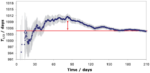
Figure 7. Daily updates of fitted 55Fe half-life values to a growing data set. Intermediate values are discrepant with the final result, which proves that the uncertainty from the least-squares fit is unrealistically low [74].
Download figure:
Standard image High-resolution imageWhereas the effect of stochastic errors on the fitted half-life reduces roughly proportionally to the square root of the number of measurements, there is no such reduction factor to correlated errors which affect the fitted half-life without leaving much of a trace in the residuals. For example, over- or undercompensated dead time losses follow an exponential behaviour with time which cannot be distinguished from the exponential shape of the decay curve. Similarly, the effect of slow geometric changes in an ionisation chamber remained unnoticed for years, but has led to systematic discrepancies in literature [72, 75].
4.3. Spectral deconvolution
Gamma-ray [47] and alpha-particle spectrometry [76] are typical examples in which quantitative information is extracted from a histogram using deconvolution software [77, 78]. Peaks in the spectrum are particular to the decay of a radionuclide and their area is proportional to the measured activity. They have to be separated from background and continuum signals, as well as from interfering peaks of other radionuclides. Heuristic peak models are designed to represent the spectral peak shapes without bias [19, 20] and matched to the spectrum with least-squares fitting algorithms.
Whereas spectra can be successfully analysed by software packages, it generally takes human experience to oversee and correct the results from automated routines. Tests have shown that programs could analyse peak areas of singlet peaks in γ-ray spectra rather well, but statistical control was found to be lacking in the analysis of peak positions and doublet peak areas [77]. Near the decision threshold, peaks are not always correctly identified and their fitted area may be biased [79]. Tested alpha deconvolution programs exhibited lack of statistical control in reported peak areas (and energies), especially where the deconvolution of multiplets or analysis of spectra with very good statistics were concerned [78]. A more elaborate treatment of spectral interference has been proposed [76].
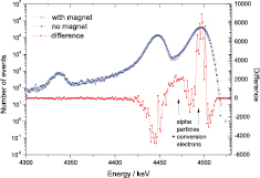
Recent developments in alpha spectrometry revealed that small spectral distortions of the peak shape lead to larger errors in relative peak areas than expected [28, 76]. Figure 8 shows two high-resolution alpha spectra of 236U [80] taken with the same detector, but once with a magnet system which eliminates interfering conversion electrons co-emitted with the alpha particles. Due to the slight difference in spectral shape, barely visible with the eye, the alpha emission probabilities derived from the spectrum without magnet are significantly wrong, even after a theoretical correction for coincidence effects [76, 80].
Figure 8. Difference between 236U alpha spectrum taken without and with magnet system (using a 150 mm2 PIPS detector), showing how coincidences with conversion electrons depopulates the second peak and broadens the highest peak. The peak distortions compromise the outcome of spectral deconvolution [80].
Download figure:
Standard image High-resolution image
5. Conclusions
Science-based decision making is based on reliable measurements. The hallmark of good metrology lies not only in the accuracy of the measurement, but even more so in the correct assessment of the uncertainty on the obtained result. In the field of radionuclide metrology, the awareness about the importance of extensive uncertainty estimation has grown over the decades. The publication of the GUM has contributed to uniformity in the terminology and the algorithms used to express uncertainty. Nevertheless, persisting discrepancies in intercomparisons and among published nuclear decay data are reminders that complete statistical control has not been achieved.
Evidence shows that uncertainty estimations differ greatly from one laboratory to another. One of the reasons is that advanced measurement methods rely on complex modelling which makes it inherently impossible to translate the entire measurement model for performing an activity assay into a single equation with a closed form. Uncertainty propagation of an immense number of parameters, from decay schemes, nuclear and atomic data, reaction cross sections, geometry and chemical composition, response of the detector, and nuclear counting is difficult to realise in practice. Another class of errors is due to overconfidence in analytical models to represent physical reality, since small imperfections can have unforeseen consequences.
Weapons against overconfidence are in-depth study of the fundamental properties of the measurand, extensive sensitivity analysis, long-term investment in mastering metrological techniques, repeatability tests, redundancy of methods, training and education. The radionuclide metrology community increases awareness about uncertainties by fostering regular intercomparisons, publishing a dedicated monograph with in-depth discussion of uncertainty components for each standardisation technique, emphasising uncertainty in graphical representations of measurement data through PomPlots, and applying the power-moderated mean to derive a robust reference value from discrepant data sets.