

Abstract
Gravity meters must be aligned with the local gravity at any location on the surface of the earth in order to measure the full amplitude of the gravity vector. The gravitational force on the sensitive component of the gravity meter decreases by the cosine of the angle between the measurement axis and the local gravity vector. Most gravity meters incorporate two horizontal orthogonal levels to orient the gravity meter for a maximum gravity reading. In order to calculate a gravity correction it is often necessary to estimate the overall angular deviation between the gravity meter and the local gravity vector using two measured horizontal tilt meters. Typically this is done assuming that the two horizontal angles are independent and that the product of the cosines of the horizontal tilts is equivalent to the cosine of the overall deviation. These approximations, however, break down at large angles. This paper derives analytic formulae to transform angles measured by two orthogonal tilt meters into the vertical deviation of the third orthogonal axis. The equations can be used to calibrate the tilt sensors attached to the gravity meter or provide a correction for a gravity meter used in an off-of-level condition.
Export citation and abstract BibTeX RIS

Original content from this work may be used under the terms of the Creative Commons Attribution 3.0 licence. Any further distribution of this work must maintain attribution to the author(s) and the title of the work, journal citation and DOI.
Introduction
Terrestrial gravity meters measure the gravitational acceleration near the surface of the earth. Some of these instruments, called absolute gravity meters, monitor the trajectory of a freely falling proof mass consisting of a falling reflector [1] or even cooled atoms [2], using sensitive laser or atom interferometer. A freely falling mass falls along a vector nominally pointing at the centre of the earth but perturbed by the non-spherical shape of the earth due to rotation and other nearby mass anomalies. The geodesic along which a mass falls freely near the surface of the earth in the absence of other forces is called the local vertical, which includes all gravitational forces from the earth, sun, moon, and other planets and even non-inertial forces such as the rotation of the earth. The interferometer used to measure the displacement of the freely falling proof mass must be aligned with the local vertical to correctly measure the position. These instruments suffer from a cosine error between the angle of the local vertical and the sensitive axis of the interferometer.
The most common gravity meters, called relative gravity meters, do not measure the acceleration of freely falling proof masses but rather measure the static force of gravity on a proof mass using an elastic element. A metal or quartz spring, or even an electrostatic or superconducting magnetic force, can be used to provide the force feedback. These instruments typically constrain any motion of the proof mass to a single axis along which the force is measured. When the sensitive axis of the gravity meter is aligned with the local gravity, the measured gravity typically has a maximum value. The measured gravity force is reduced by the cosine of the angle between the sensitive axis of the gravity meter with the true vertical defined by local gravity.
The superconducting gravity meter [3] (SG) has another larger tilt-error caused by the horizontal motion of the superconducting sphere in the magnetic field as the vertical angle of the sensor is varied. It turns out that this error is also quadratic in angle but has the opposite sign of the usual gravity reduction so that the SG is typically levelled to a minimum gravity value [4–6].
The measured gravity value for most gravity meters (other than the SG) is therefore given by

where the angle,  , is the measured angle between the local value of gravity and the vertical axis of the gravity meter. The value,
  , is the local value of maximum gravity in gravity units (m s−2). The superconducting gravity meter also has a quadratic dependence on the deviation so equation (1) is still approximately valid as long as g0 is the appropriate (negative) constant to describe the combination of the magnetic field error and gravity error.
Calibration of tilt meters in a gravity meter
It is common practice to attach two horizontal orthogonally aligned tilt meters to the gravity to determine when the gravity meter axis is vertical. Assuming that the two orthogonal, nominally 'horizontal', tilt meters measure angles from the horizontal axes given by X and Y, it is common practice to approximate the cosine of the angular deviation as a product of the cosines of the two horizontal tilt-meter angles,  .
.
This formula works well for small angles and is quite convenient because the two angular factors are independent. When expanded in terms of small angles to the second order, the cosine terms becomes:

In practice, one must determine the two offsets for each tilt meter, X0 and Y0. The values of these offsets for each tilt meter are given by the measured angles when gravity reading is at an extremum. Note that these offsets can be determined even if the gravity sensor or the tilt sensors are not calibrated.
If the gravity sensor is calibrated, one can transfer this calibration to the two tilt meters. To see this, consider a slightly more complicated expression for the angular sensitivity of the gravity meter that includes both the offset for each tilt meter as well as the two tilt meter calibration factors, CX and CY.

The measured gravity signal,  , as a function of the deviation,
  , between the sensitive axis of the gravity meter and the local vertical can be written using a Taylor expansion of linear and quadratic terms for small angles, X and Y:

where the two offsets are given by:
and the two calibration constants for the tilt meters are:
These equations provide a mathematical model that can be used to fit gravity measurements at different angles in both axes to determine the two angular offsets for maximum gravity and also the calibration constants for each tilt meter. The offsets will have the same units as the tilt-meter readout. For example, if the tilt-meters provide a voltage level, then the offsets will be the voltage levels for maximum gravity on each tilt meter. The calibration constants will have units of radians per tilt-meter unit.
This or a similar procedure is done on most gravity meters that rely on external tilt meters to level it prior to being used. Often only one axis is calibrated at a time but with the advent of fast computers it is quite easy to least squares fit data on both axes simultaneously.
These parabolic relationships between gravity measurements and tilt-meter readings have been used for as long as gravity meters have been manufactured because they provide a simple method for aligning the tilt meters with the gravity sensor.
Once the tilt meter calibrations have been performed on a particular gravity meter and the offsets for maximum gravity have been determined, they can be used to provide an off-level correction. This can be useful if one wants to save time on a survey and quickly adjust the feet of a gravity meter to an approximately level condition and then use the measured tilt readings to correct the gravity meter to its maximum gravity value. It can also be useful if a gravity meter is sitting in a fixed location and a long time series is recorded. The tilt-correction can be used to adjust the recorded gravity for tilts in the floor.
Equating the cosine of the angular deviation of the sensitive axis of the gravity meter from the local vertical with the simple product of the cosines of the two horizontal tilt meter readings provides a very nice justification for the parabolic response of a gravity meter to the measured tilts. However, equation (2) is only valid for small angles. In practice, these approximations are valid for most cases but for completeness, it is useful to derive an analytically correct expression for the tilt error that can be used at any angle.
Derivation of vertical deviation as a function of measured tilts
The algebraic mechanics of this inherently 3D problem are most easily handled using rotation matrices. Consider a gravity meter whose sensitive axis is initially aligned with the vertical, z-axis, and the two tilt meters attached to the gravity meter are aligned with the horizontal x and y axes. For simplicity, we will refer to these as the X-tilt meter and Y tilt-meter, respectively. It is assumed that the initial x, y, and z axes are stationary and fixed to the earth and the z axis is aligned with the local gravity vector.
There are many ways to rotate a gravity meter to an arbitrary orientation using two rotations. One of the simplest sequences is to first rotate the gravity meter around the Z axis by θ and then around the original X axis by another angle  . The final deviation of the gravity meter from the vertical after these two rotations is clearly
  since the first rotation does not affect the inclination of the gravity meter. Figure 1 shows an idealized gravity meter with two bubble levels that has been rotated first around the z axis and then around the x axis. The z axis is aligned with gravity.
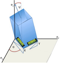
Figure 1. Rotation of gravity meter around two axis (first z and then x).
Download figure:
Standard image High-resolution imageThe question we want to answer is how to calculate the angle of deviation,  , using the measured tilts from the tilt-meters attached to the gravity meter. We can answer this by expressing the three axes of the gravity meter after the two rotations in the original un-rotated frame aligned with gravity.
After the first rotation, θ, around the vertical z axis, the three axes attached to the gravity meter are rotated in the stationary frame using,

The unit vectors aligned with the gravity meter after rotation are found by multiplying the rotation matrix by the unit vectors in the un-rotated frame, (i.e.  )
)
We can apply a second rotation of angle  to the gravity meter around the original X axis using the rotation matrix,

The sign of both rotations are consistent with a right hand rule. The unit vectors attached to the gravity meter after the two rotations can be expressed in the original frame by applying a compound rotation matrix,  , given by the product of the two individual rotation matrices to the original unit vectors aligned with
  ,
,  and
and  . The compound rotation matrix linking the doubly rotated reference frame to the original stationary frame is given by

Each column of the compound rotation matrix, R, gives the components of the corresponding unit vector attached to the twice rotated gravity meter expressed in the original stationary frame that is aligned with gravity.
What remains to be done is to find the angles read by the two tilt meters attached to the gravity meter. A dot product of the unit vectors attached to the gravity meter with the original z axis provides the cosine of the angle between that unit vector and vertical. These three dot products are given by the entries in the third row in the compound matrix. The last entry in the matrix, for example shows that the sensitive axis of the gravity meter is rotated from true vertical by the angle  .
.
The tilt meters attached to the gravity meter measure the deviation of each sensor from the original horizontal plane. If we call the two measured tilt angles of the gravity meter, X and Y. The sine of these angles is equivalent to the dot product of the unit vector aligned with each tilt meter and the true vertical axis aligned with the original z unit vector. Thus,  and similarly
  . The gravity correction is sensitive to the cosine of the deviation,
  , of the gravity meter axis from the local vertical.
This gives two parametric equations in two rotation angles, θ and  , that while never measured in practice, link the two measured tilt angles, X and Y, with the deviation angle,
  , of the gravity meter from the local vertical.

Eliminating the uninteresting angle θ, we arrive at a closed form expression linking the deviation of the vertical gravity meter axis from the local gravity, in terms of the two measured tilts from the tilt meters attached to the gravity meter,

An equivalent expression relating horizontal tilts to the measured reduction in gravity is

Experimental verification
The closed formula, equation (11), for the deviation was checked using a three axis inclinometer chip, ADXL312 by Analog Devices, mounted on two orthogonal coupled rotation stages as shown in figure 2. The inclinometer chip was mounted to a printed circuit board that was then mounted to the smaller of the two rotation stages. Initially, the large rotation stage was rotated so that the circuit board and inclinometer was horizontal. This position corresponded to zero degrees of inclination,  . Rotation of the small stage corresponds to the angle θ discussed above for rotations around the vertical (when
  ). The horizontal axes of the inclinometer chip were aligned with the edges of the circuit board.

Figure 2. Experimental setup.
Download figure:
Standard image High-resolution imageThis setup allowed us to directly vary and measure the two parametric rotation angles, θ and  , using the two rotation stages. The Z deviation from vertical read from the inclinometer chip could be directly compared to the angle read off of the large rotation stage since they should be equal (
 ). The horizontal inclinations X and Y from the chip could then be used to calculate the angles, θ and
  , on both rotation stages using equation (10). Finally, we could calculate the vertical deviation of the chip (θ or Z) with the prediction using the measured X and Y inclinations with either the usual approximation,
  or that given by equation (11) derived above.
The results of a comparison of the difference,  , between the approximate formula (equation (2)) and the exact formula (equation (11)) for calculating the deviation from vertical,
  , using the horizontal tilts, X and Y, are shown in Figure 3 for an initial rotation, θ = 45°. The angle of the deviation from vertical measured from the rotation stage,
  , is plotted along the x axis and the difference in the deviation from vertical calculated from the horizontal deviation using the two formulae are shown on the y axis. The measured values of

Figure 3. Error,  , between correct deviation angle,
  , and the approximation
  .
.
Download figure:
Standard image High-resolution image
The plot shows that the approximation,  , while valid at small angles breaks down at large angles. The two can by as much as 30° at a deviation of 90°.
For gravity meters, the error introduced by the approximation is more interesting for smaller angles near 1°. The second column of table 1 shows the gravity correction, δg, for tilts of a gravity meter from vertical. The third and fourth columns give the errors in angle and gravity correction by using the approximation given in equation (2). The gravity correction error is 11 μGal for 1° and increases to about 1 mGal at 3°.
Table 1. Deviation from vertical and gravity error.
Deviation  (degrees) (degrees) |
Gravity correction δg (mGal) | Error | |
|---|---|---|---|
| Angle (arc-second) | Gravity (mGal) | ||
| 1 | 149.259 | 0.12 | 0.011 |
| 2 | 596.99 | 0.97 | 0.182 |
| 3 | 1343.056 | 3.29 | 0.92 |
Conclusions
The tilt correction, δg, for a gravity meter that has been tilted by about 9 arc-sec (~45 μrad) is approximately 1 part per billion of the local value of gravity (1 μGal) and increases quadratically with the deviation for small angles. The error is a result of the cosine dependence of the measured gravity value on the angle between the sensitive axis of the gravity meter and the local vertical given in equation (1). The cosine of the vertical deviation of a gravity meter is often estimated as a product of the cosines of two measured horizontal tilt angles,  . A Taylor expansion of this expression in two dimensions shows that to second order, the overall gravity error is an uncoupled quadratic function of both angles. This fact is quite useful for finding the tilt offsets at which the gravity meter measures a maximum gravity signal. This methodology has been in use by gravity meter users for many years and works well for small angles. We presented formulae that can be used to perform a simultaneous least-squares solution for measured gravity as a function of tilts in two dimensions. This procedure provides the offset for each tilt meter for which gravity is a maximum. It also calibrates the tilt meters as long as the gravity meter is first calibrated in terms of gravity.
At large angles, the cosine of the deviation of the vertical axis of the gravity meter from local vertical begins to diverge from the simple product of the cosines of each horizontal tilt meter. Rotation matrices were employed to find an exact analytic expression valid for all angles.
We were able to confirm experimentally that the exact expression matched measurements with a three-axis inclinometer even at large angles. At current levels of gravity meter sensitivity, the exact expressions for the tilt-correction of gravity will have application at tilts of around 1°.
These formulae also have use in other applications such as borehole gravity where two horizontal tilt meters attached to the sonde of a borehole instrument can be used to infer the deviation of the well as the tool is lowered into the ground.