


ABSTRACT
We construct revised response functions for the Atmospheric Imaging Assembly (AIA) using the new atomic data, ionization equilibria, and coronal abundances available in CHIANTI 7.1. We then use these response functions in multithermal analysis of coronal loops, which allows us to determine a specific cross-field temperature distribution without ad hoc assumptions. Our method uses data from the six coronal filters and the Monte Carlo solutions available from our differential emission measure (DEM) analysis. The resulting temperature distributions are not consistent with isothermal plasma. Therefore, the observed loops cannot be modeled as single flux tubes and must be composed of a collection of magnetic strands. This result is now supported by observations from the High-resolution Coronal Imager, which show fine-scale braiding of coronal strands that are reconnecting and releasing energy. Multithermal analysis is one of the major scientific goals of AIA, and these results represent an important step toward the successful achievement of that goal. As AIA DEM analysis becomes more straightforward, the solar community will be able to take full advantage of the state-of-the-art spatial, temporal, and temperature resolution of the instrument.
Export citation and abstract BibTeX RIS
1. INTRODUCTION
The key to discriminating among different coronal heating models is to identify distinguishing observables. One such observable is the cross-field temperature distribution. If this distribution is consistent with isothermal plasma, the observed loop could be modeled as a single flux tube. If this is not the case, however, the loop may be composed of a collection of tangled magnetic strands. Here, we apply the definition that a loop is a distinct configuration in an observation and a strand is an elementary flux tube where the physical properties of temperature and density are constantly perpendicular to the field lines. Klimchuk (2006) showed that certain classes of corona heating models apply only if loops are multi-stranded and could be ruled out if loops are revealed to be single flux tubes.
The Atmospheric Imaging Assembly (AIA; see Lemen et al. 2012) on the Solar Dynamics Observatory is a state-of-the-art imager with the potential to do unprecedented time-dependent multithermal analysis at every pixel. The EUV filters peak at different temperatures, making AIA ideal for determining the cross-field temperature distribution. Recent results, however, have identified missing lines in the CHIANTI atomic physics database, which is used to construct the instrument response functions (see, e.g., O'Dwyer et al. 2010; Del Zanna et al. 2011; Testa et al. 2012). The most serious problems appeared to be with the 131 and 94 Å channels, but there was significant improvement for the 94 Å passband when the two Fe ix lines at 93.59 Å and 94.07 Å identified in the laboratory by Lepson et al. (2002) were included in the calculation of the AIA response (Foster & Testa 2011).
Schmelz et al. (2011a, 2011c) analyzed 12 cool and 12 warm coronal loops from several active regions observed by AIA. The cooler loops were selected in the 171 Å images, which has a peak response temperature of log T = 5.8. The warmer loops were selected in the 211 Å images, which has a peak response at log T = 6.3. Their isothermal and multithermal analysis revealed that several of these loops appeared to have unrealistically broad temperature distributions, with significant emission measure at log T ≈ 6.8–7.0. Such high temperatures were inconsistent with the results of spectrometers for quiescent loops. The biggest problem for the temperature analysis appeared to be related to the AIA 131 Å channel. This problem was originally attributed to missing low-temperature lines, but missing lines alone could not explain the results of Schmelz et al. (2013a). They did differential emission measure (DEM) analysis using simultaneous AIA and Hinode EUV Imaging Spectrometer (EIS; Culhane et al. 2007) observations of six X-ray bright points. Their results not only supported the conclusion that CHIANTI version 7 was incomplete near 131 Å, but also suggested that the peak temperature of the Fe viii emissivity and response functions were warmer than the current value of log T = 5.7.
CHIANTI version 7.1 (Dere et al. 1997; Landi et al. 2013) has added numerous configurations to the atomic models of Fe viii to xiv. These were calculated using the flexible atomic code under the distorted wave approximation. These configurations are responsible for many spectral lines in the 50–170 Å wavelength range, which contribute significantly to the 131 and 94 Å AIA passbands. In addition, improved recombination rates are used to provide a new set of ionization equilibrium calculations, where the peak temperature of the Fe viii is slightly higher. CHIANTI 7.1 also provided the new set of coronal element abundances from Schmelz et al. (2012), which is an update the hybrid abundances of Fludra & Schmelz (1999).
In this paper, we constructed synthetic solar spectra with the new atomic data, ionization equilibria, and coronal abundances available in CHIANTI 7.1. We convolved these spectra with the AIA effective areas in SolarSoft to create an updated set of AIA response functions. It is reassuring that these new response functions are similar to the empirically revised response functions determined by Schmelz et al. (2013a) during the AIA–EIS DEM analysis of the bright points mentioned above. We have applied these new CHIANTI 7.1 response functions to AIA loop data in order to obtain the cross-field temperature distribution and determine if the results are consistent with single flux tubes or if multiple strands are required.
2. OBSERVATIONS
The AIA coronal channels are each dominated by an iron emission line of a different ionization stage, from Fe viii to Fe xviii (plus flare lines). This feature makes AIA not only a state-of-the-art imager, but also gives it better temperature resolution than any of its non-spectrometer predecessors. It has the ability to do time-dependent multithermal analysis at every pixel on scales short compared to the radiative and conductive cooling times and, therefore, to add significantly to our knowledge of solar coronal physics. Boerner et al. (2012) presented the initial photometric calibration of AIA, which was based on preflight measurements of the telescope components. They also described the characterization of the instrument performance and calculated the response functions.
AIA has a full-disk field-of-view, a 1.5 arcsec spatial resolution, and a 12 s temporal resolution. It has six coronal bandpasses centered on specific iron lines: Fe viii at 131 Å, Fe ix at 171 Å, Fe xii at 193 Å, Fe xiv at 211 Å, Fe xvi at 335 Å, and Fe xviii at 94 Å. Please see Lemen et al. (2012) and Boerner et al. (2012) for details. The AIA response functions have units of DN s−1 pixel−1 per unit emission measure and are shown in Figure 1. The dashed curves show the original results calculated with CHIANTI 7 and the solid curves show the new results constructed with CHIANTI 7.1.
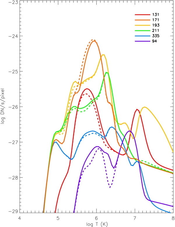
Figure 1. The six AIA coronal response functions showing the sensitivity of each filter as a function of temperature. The dashed curves show the original results calculated with CHIANTI 7 and the solid curves show the new results constructed with CHIANTI 7.1. Both sets of curves use the coronal abundances of Schmelz et al. (2012).
Download figure:
Standard image High-resolution imageIn this paper, we have analyzed 12 different loop segments selected from six different active regions, which were observed by AIA on five different dates from 2010 July to 2011 September. Details for each observation, including the date, time, active region number, and solar coordinates are listed in Table 1. Also listed there is a qualitative description of each loop segment as it appears in each of the different AIA filters. The loops chosen for DEM analysis needed to be visible in at least three AIA filters and have a nearby clean area appropriate for background subtraction.
Table 1. AIA Loop Data Sets
| ID | Date | AR | Position | 131 Å | 171 Å | 193 Å | 211 Å | 335 Å | 94 Å |
|---|---|---|---|---|---|---|---|---|---|
| Time | 3:00:45 | 3:00:47 | 3:00:42 | 3:00:48 | 3:00:51 | 3:00:44 | |||
| a | 15-Jul-10 | 11087 | N20W06 | Barely visible | Clearly visible | Clearly visible | Clearly visible | Not visible | Not visible |
| b | 15-Jul-10 | 11087 | N20W06 | Barely visible | Visible | Visible | Clearly visible | Barely visible | Not visible |
| Time | 17:00:33 | 17:00:24 | 17:00:31 | 17:00:24 | 17:00:27 | 17:00:20 | |||
| c | 27-Jul-10 | 11089 | S24W35 | Visible | Visible | Visible | Visible | Not visible | Not visible |
| d | 27-Jul-10 | 11089 | S24W35 | Visible | Clearly visible | Visible | Barely visible | Not visible | Not visible |
| Time | 17:00:09 | 17:00:00 | 17:00:07 | 17:00:00 | 17:00:03 | 17:00:02 | |||
| e | 10-Aug-10 | 11093 | N10W12 | Barely visible | Visible | Visible | Visible | Not visible | Not visible |
| Time | 0:01:09 | 0:01:12 | 0:01:07 | 0:01:12 | 0:01:15 | 0:01:14 | |||
| f | 15-Feb-11 | 11159 | N19W21 | Not visible | Clearly visible | Visible | Barely visible | Not visible | Not visible |
| g | 15-Feb-11 | 11158 | S21W21 | Visible | Clearly visible | Barely visible | Barely visible | Not visible | Not visible |
| h | 15-Feb-11 | 11158 | S21W21 | Barely visible | Visible | Barely visible | Not visible | Not visible | Not visible |
| i | 15-Feb-11 | 11158 | S21W21 | Visible | Clearly visible | Barely visible | Barely visible | Not visible | Not visible |
| j | 15-Feb-11 | 11158 | S21W21 | Not visible | Visible | Visible | Barely visible | Not visible | Not visible |
| k | 15-Feb-11 | 11158 | S21W21 | Barely visible | Visible | Barely visible | Barely visible | Not visible | Not visible |
| Time | 22:48:09 | 22:48:00 | 22:48:07 | 22:48:01 | 22:48:03 | 22:48:02 | |||
| l | 15-Sep-11 | 11289 | N24W37 | Visible | Visible | Visible | Barely visible | Barely visible | Not visible |
Download table as: ASCIITypeset image
Figure 2 shows the 171 Å AIA images for each of the active regions. The loop targets are outlined with white boxes and labeled with letters corresponding to those listed in Table 1. The 12 panels of Figure 3 show close-up images of each loop segment, where the small boxes show the loop targets in red and the associated background area in white.

Figure 2. Images of the observed active regions from the 171 Å channel of AIA where each loop segment chosen for DEM analysis is marked and labeled. The main ion contributing to this filter is Fe ix with a peak formation temperature of Log T = 5.8. (a) AR 11087 on 2010 July 15; (b) AR 11089 on 2010 July 27; (c) AR 11093 on 2010 August 10; (d) AR 11159 on 2011 February 15; (e) AR 11158 on 2011 February 15; and (f) AR 11289 on 2011 September 15.
Download figure:
Standard image High-resolution image
Figure 3. Closeup 171 Å AIA images of the 12 loops selected for analysis. The red boxes highlight the loop segment under investigation and white boxes outline the selected background area. Please note: the red boxes outline the loop segment we analyzed, but are not meant to represent the collection of loop pixels we averaged. If we outline only the selected pixels along the spine of the loop, we actually mask the structures that we are trying to highlight.
Download figure:
Standard image High-resolution imageOur analysis is similar to that described by Schmelz et al. (2011a, 2011c). We co-aligned the six AIA coronal images for each observation and chose 10 pixels along the spine of the loop, which are inside the red boxes in Figure 3, and 10 nearby background pixels, which are inside the white boxes in Figure 3. We then averaged the intensities in each group and computed the standard deviations. We normalized the background-subtracted averages and uncertainties by dividing by the exposure times. The resulting units are Data Numbers s−1.
3. ANALYSIS
The intensity for each AIA passband is proportional to ∑ Resp(T) × DEM(T) Δ T, where Resp(T) is the response function (DN s−1 pixel−1 per unit emission measure) and DEM is the differential emission measure (cm−5 K−1). The multithermal analysis described in this paper uses XRT_dem_iterative2 (Weber et al. 2004; Schmelz et al. 2009), a forward-fitting routine which uses a best-guess DEM that is then folded through the AIA response functions to generate a set of predicted intensities. This process is then repeated to minimize χ2 for the predicted-to-observed intensity ratios. This routine interpolates the DEM function using several spline points that are manipulated by mpfit.pro, which uses a Levenberg–Marquardt least-squares minimization. A useful option in XRT_dem_iterative2 is the Monte-Carlo iterations, where the observed intensity in each filter is varied randomly using a Gaussian distribution where the observed intensity is the centroid and the uncertainty is the width. The program is run again with each new set of values, and the tightness of the resulting solutions can be used as a measure of goodness-of-fit on the DEM result. For additional XRT_dem_iterative2 analysis, please see Schmelz et al. (2010) and Winebarger et al. (2011).
The DEM results from xrt_dem_iterative2 for each background-subtracted loop segment are shown in Figure 4. These curves are made with data from all six AIA coronal channels and the new CHIANTI 7.1 response functions. The red dashes show the 100 Monte-Carlo realizations. The vertical spread in the Monte Carlos gives an indication of how well (or not well) constrained the solution is in a particular temperature range. For example, the Monte Carlo solutions for all the loops are well constrained near the peak of the distribution. In some cases, the vertical spread gets larger at the highest (e.g., loop i) and lowest (e.g, loop h) temperatures, indicating that the solution is not as well determined away from the DEM peak. Increasing the signal to noise by averaging over more pixels, increasing the AIA exposure time, or averaging multiple AIA images in each filter could help reduce the range of the Monte Carlos and pin down the best DEM result.
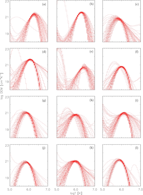
Figure 4. DEM results from xrt_dem_iterative2 for each loop segment depicted in Figure 3 and listed in Table 1. The red dashed histograms represent the Monte Carlos, where the vertical range indicates how well-constrained the DEM solution is in a particular temperature bin.
Download figure:
Standard image High-resolution imageSome loops (e.g., loop e) are poorly constrained on the cool temperature end. As a result, emission measure leaks out into the lowest temperature bins where it probably does not belong. The more reliable response function for the 131 Å AIA filter provided by CHIANTI 7.1 helps significantly with this problem, which was much worse with CHIANTI 7.0. Here, despite the leaky cool emission measure, a reasonable DEM solution for this loop segment is discernible in Figure 4(e). These results are much more encouraging than those published by Schmelz et al. (2011c), who were forced to drop the 131 Å data. There, the uncertainties were so large that, as a result, the DEMs were not well defined. The response functions generated with CHIANTI 7.1 data represent a significant improvement.
Figure 5 shows the log of the predicted-to-observed intensity ratios for the lowest reduced χ2 solution of the Monte Carlos plotted in the equivalent panel of Figure 4. The diamonds show the six AIA coronal channels in order of increasing wavelength (1) 94 Å, (2) 131 Å, (3) 171 Å, (4) 193 Å, (5) 211 Å, and (6) 335 Å, which also corresponds to the effective temperature order for these loop segments. Ideally, all the data points would fall along the horizontal dashed line at zero, within uncertainties. These results indicate that the DEM solutions for the loop segments are excellent, with reduced χ2 ≈ 1.0 in all cases, except for loop d with reduced χ2 = 2.2.

Figure 5. Log of the predicted-to-observed intensity ratios for the lowest reduced χ2 solution of the Monte Carlos from Figure 4. The diamonds show the six AIA coronal channels in order of increasing wavelength (1) 94 Å, (2) 131 Å, (3) 171 Å, (4) 193 Å, (5) 211 Å, and (6) 335 Å, which corresponds to the effective temperature order for these loop segments. The DEM solutions for the loop segments are excellent, with χ2 ≈ 1.0 in all cases, except for loop d with χ2 = 2.2.
Download figure:
Standard image High-resolution image
Significant hot (log T ∼ 6.8) emission measure, as indicated by many of the Monte Carlos in, e.g., loop i is not a reliable result from this analysis. This is most likely not related to a problem with the AIA response functions or to missing lines in the CHIANTI atomic physics database. Rather, it appears to be connected to what Winebarger et al. (2012) refer to as the blind spot in DEM analysis. Although they were using EIS and XRT temperature measurements, the same principle applies here. In effect, the Fe xvi 335 Å AIA channel and/or the Fe xviii component of the 94 Å AIA channel do not provide a strong enough high-temperature constraint for the loop DEM analysis, especially after the required background subtraction. One possible solution for this problem is to use simultaneous XRT data in conjunction with the AIA images to effectively block off this area of DEM space and force all the Monte Carlos to lower temperatures.
4. DISCUSSION
Previous work by Schmelz et al. (2011a, 2011c) looked at isothermal and multithermal analyses of coronal loops observed with AIA. They wanted to know if AIA could determine a unique cross-field temperature distribution without ad hoc assumptions. Since they needed to see the full family of solutions that could reproduce the observed AIA intensities, they used xrt_dem_iterative2 with the option of Monte Carlo solutions. The problem they encountered was with the default AIA response functions. The problems were so severe for the AIA 131 Å filter that it had to be dropped from the analysis. Without this filter to provide a cool-temperature constraint in the multithermal analysis, the DEM results were disappointing. The Monte Carlo solutions for many of the loops tested did not converge. With the revised response functions used here, however, the multithermal analysis of coronal loops using AIA data appears much more promising.
The AIA DEM results presented here are consistent with those from other instruments, including the Solar and Heliospheric Observatory (SOHO) Coronal Diagnostics Spectrometer (CDS; see, e.g., Schmelz et al. 2001, 2007) and the Hinode EUV Imaging Spectrometer (EIS; see, e.g., Warren et al. 2008; Schmelz et al. 2010, 2011b). This agreement with results from spectrometers bodes well for the future of AIA multithermal analysis. The caveat, however, is that the AIA response functions must reflect the properties of the coronal plasma as accurately as possible, and not just our current knowledge of the plasma. CHIANTI 7.1 appears to do a good job of successfully modeling the plasma that contributes significantly to the AIA coronal response functions.
Successful DEM loop analysis using AIA data, like the results presented in this paper, are an important extension of these previous results from CDS and EIS. This value is a consequence of the fundamental differences between imagers and spectrometers. Where spectrometers have excellent spectral (and therefore temperature) resolution that is essential for DEM analysis, they also have poor spatial resolution and slow time cadence compared with imagers. The analysis can also be tedious, resulting in only a few meticulously analyzed loops which must be assumed to be in a quiescent state. Imagers, on the other hand, have traditionally had poor temperature resolution, but have benefited from excellent spatial resolution and fast time cadence compared with spectrometers. Over time, spectrometers have gotten better spatial resolution (e.g., SOHO CDS > Hinode EIS), while imagers have gotten better temperature resolution (e.g., Yohkoh SXT > Hinode XRT).
The original controversy over the results of loop cross-field temperature distributions helped spark the series of Coronal Loop Workshops (Paris 2002, Palermo 2004, Santorini 2007, Florence 2009, and Mallorca 2011). One point of contention was that filter ratios analysis with TRACE data gave (by design) isothermal values while DEM analysis of CDS spectra gave multithermal results. The DEM results were not consistent with loops modeled as single flux tubes. Critics blamed the differences on the shortcomings of CDS, primarily that the pixel size was significantly larger than that of TRACE. This criticism was in fact true—CDS could indeed have been averaging over multiple features that could have been seen by TRACE as a single loop. The new loop studies presented in this paper, however, seem to contradict these old critics. For the first time, AIA brings the best features of imagers together with those of spectrometers—where spectrometers are forced to sacrifice spatial and/or temporal resolution for spectral resolution, AIA can maintain state-of-the-art spatial and temporal resolution with excellent coronal temperature coverage. Reliable DEM analysis can be done at every AIA pixel, not only for loops and other quiescent features, but for dynamic events as well.
There are certainly loops and loop segments in AIA images that appear in only one filter and are therefore consistent with isothermal plasma. Such loops have also been analyzed using spectrometer data (see, e.g., Del Zanna & Mason 2003; Schmelz et al. 2007; Brooks et al. 2011). These loops could be formed of a single strand, which would imply we are currently resolving the corona, or they could be formed of many sub-resolution strands which are currently cooling through a single AIA passband (see, e.g., Winebarger et al. 2003; Viall & Klimchuk 2011). The loops analyzed here, however, are not isothermal and cannot be formed of a single strand. They appear in at least three filters, and we are not able to reproduce the AIA intensities with an isothermal model. The multithermal analysis in Figure 4 shows DEM results that are neither isothermal nor extremely broad.
Recent analysis finds some evidence that warmer loops require broader DEMs (Schmelz et al. 2013b). Loops selected in images of warm coronal lines like Si xii and Fe xv or XRT images tend to have to have broader DEMs (Schmelz & Martens 2006; Schmelz et al. 2010, 2011b). Loops selected in images of somewhat cooler lines, usually Fe xii, have DEMs that are less broad but still not isothermal (Warren et al. 2008; Schmelz et al. 2013b), and many loops that are selected in images of cool coronal lines like Mg ix and Fe ix show narrow DEMs and even isothermal plasma (Del Zanna & Mason 2003; Schmelz et al. 2007; Brooks et al. 2011). If the observed loops are cooling (see, e.g., Winebarger & Warren 2005), then it would make intuitive sense that loops that have had time to cool to temperatures below a million degrees might not have significant associated hotter plasma. AIA is ideal for investigating this problem. The evolution of loops can be observed as they cool through the AIA passbands, and the DEMs can be constructed reliably with the new AIA response functions.
The heating of loops with multithermal cross-field temperatures can be impulsive or steady, but impulsive heating is a more straightforward interpretation. If loops are multi-stranded, and if the strands are heated by nanoflares that occur over a finite window of time (a nanoflare storm), then the strands will be in different stages of cooling, and the loop will be multithermal. Isothermal loops can also be heated by nanoflares, but the nanoflares must all go off at approximately the same time, i.e., the nanoflare storm must be of short duration (Klimchuk 2009). Steady heating can produce multithermal loops, but the heating rate must be different in the different strands. It is not obvious why this would be the case. Thus, the existence of multithermal loops does not prove that nanoflares heat the corona, but this is the simplest explanation. In any case, it does provide an observational constraint that all feasible coronal heating models will have to explain.
5. CONCLUSIONS
We constructed synthetic solar spectra with the new atomic data, ionization equilibria, and coronal abundances available in CHIANTI 7.1. We convolved these spectra with the AIA effective areas in SolarSoft to create a new set of AIA response functions. Applying the new CHIANTI 7.1 AIA response functions to coronal loop segments has allowed us to determine a unique cross-field temperature distribution without ad hoc assumptions. Our method uses AIA data from the six coronal filters and the Monte Carlo solutions available from xrt_dem_iterative2.
The cross-field temperature distributions of our loop segments are not consistent with isothermal plasma. Therefore, the observed loops cannot be modeled as single flux tubes and must be composed of a collection of magnetic strands. This result is now supported by observations from the High-resolution Coronal Imager (Hi-C; Cirtain et al. 2013), which took 0 2 resolution images of the 1.5 MK corona on 2012 July 11. The Hi-C images show fine-scale braiding of coronal strands that are reconnecting and releasing energy. High-resolution images and multithermal analysis could provide the powerful combination of observables required to discriminate amongst different coronal heating models.
Multithermal analysis is one of the major scientific goals of AIA, and our results are an important step toward the successful achievement of this goal. We hope that AIA DEM analysis will soon become straightforward and that the solar community will be able to take full advantage of the state-of-the-art spatial, temporal, and temperature resolution of AIA.
The authors thank Jim Klimchuk (GSFC) for useful discussions and University of Memphis students Karen Paul, Runpal Dhaliwal, George Mac Christian, and Christine Fair for help with data analysis. The Atmospheric Imaging Assembly on the Solar Dynamics Observatory is part of NASA's Living with a Star program. CHIANTI is a collaborative project involving the NRL (USA), the Universities of Florence (Italy) and Cambridge (UK), and George Mason University (USA). Solar Physics Research at the University of Memphis is supported by a Hinode subcontract from NASA/SAO as well as NSF ATM-0402729.