


ABSTRACT
We studied the spatial dynamics of the flaring loop in the 2005 August 22 event using microwave (NoRH) and hard X-ray (RHESSI) observations together with complementary data from SOHO/MDI, SMART at Hida, SOHO/EIT, and TRACE. We have found that (1) the pre-flare morphology of the active region exhibits a strongly sheared arcade seen in Hα and the J-shape filament seen in EUV; (2) energy release and high-energy electron acceleration occur in a sequence along the extensive arcade; (3) the shear angle and the parallel (to the magnetic neutral line) component of the footpoint (FP) distance steadily decrease during the flare process; (4) the radio loop shrinks in length and height during the first emission peak, and later it grows; after the fourth peak the simultaneous descending of the brightest loop and formation of a new microwave loop at a higher altitude occur; (5) the hard X-ray coronal source is located higher than the microwave loop apex and shows faster upward motion; (6) the first peak on microwave time profiles is present in both the loop top and FP regions. However, the emission peaks that follow are present only in the FP regions. We conclude that after the first emission peak the acceleration site is located over the flaring arcade and particles are accelerated along magnetic field lines. We make use of the collapsing magnetic trap model to understand some observational effects.
Export citation and abstract BibTeX RIS
1. INTRODUCTION
Large two-ribbon flares are a complex phenomenon, which may be accompanied by coronal mass ejections (CMEs) and prominence eruptions (for a review see Priest & Forbes 2002). The basic model for such flares is the standard reconnection model, known as the "CSHKP" (Carmichael 1964; Sturrock 1966; Hirayama 1974; Kopp & Pneuman 1976). In this model, a flare occurs in the coronal arcade containing a prominence presumably due to the onset of reconnection below the rising arcade. A rapid eruption at the flare onset leads to the stretching of arcade field lines and the formation of the vertical current sheet above the magnetic inversion line where a production of high-energy particles and flare loops via reconnection occurs. This picture has been developed by many people, including Priest (1981), Moore et al. (1988, 1992), and Shibata (1996, 1998, 1999). This model predicts such morphological features as an expansion of the flare ribbons/footpoint distance and growth of a flare loop system.
In the past decade, special attention was paid to a new observational phenomenon: the contraction of flaring loops on the flare rising phase, which is not predicted by the standard model. The usual expansion motion of flaring loops occurs only after the contraction. This loop contraction consists of three different observational factors: converging motion of footpoints (FPs) measured using hard X-ray (HXR) emission data (Ji et al. 2004, 2006, 2007; Liu et al. 2009; Yang et al. 2009), downward motion of the loop top (LT) observed in soft X-rays (SXRs; Sui & Holman 2003; Sui et al. 2004; Li & Gan 2006; Shen et al. 2008), and shrinkage of the loop length (Li & Gan 2005; Joshi et al. 2009). This phenomenon challenges the standard flare model and triggers model improvement and development.
Microwave emission is generated through the gyrosynchrotron mechanism by mildly relativistic electrons rotating around magnetic field lines. Therefore, it is a good tracer of a flaring loop. In some flares, the whole microwave flaring loop is observed. Therefore, in these cases microwave observations with high spatial resolution allow us to study the loop length and LT height evolution, FP motion, as well as the loop's orientation during the flare process. The combination of both X-rays and microwaves is even more powerful for this type of study.
Moreover, study of a radio brightness distribution along the flaring loop gives additional information about an acceleration site location in a loop and the mildly relativistic electrons' pitch-angle distribution (Melnikov et al. 2002; Altyntsev et al. 2008; Reznikova et al. 2009). Obtained information can be used for comparison with existing flare models and acceleration mechanisms. In this paper, we have taken the opportunity for such a study with the large two-ribbon flare 2005 August 22, which was well resolved with the Nobeyama Radioheliograph and partly observed with the Ramaty High Energy Solar Spectroscopic Imager (RHESSI).
In Section 2, we examine the loop dynamics during the flare process, including spatial displacements of FPs, changing loop length and LT height, as well as some emission spatial and temporal features. We also attracted optical, Hα, and EUV images of the active region (AR) as complementary data to understand the nature of the observed dynamics. In Section 3, discovered properties are discussed. In Section 4, we summarize our results and compare the obtained findings with existing models and acceleration mechanisms.
2. OBSERVATIONS
An intense solar flare occurred on 2005 August 22 at 00:54 UT with heliographic coordinates S12°, W49°. It was one of a series of flares connected with AR NOAA 10798 and was accompanied by a high-speed CME. Figure 1 shows the emission time profiles in SXRs, microwaves, and HXRs. GOES fluxes in channels 1–8 Å (thick line) and 0.5–4 Å (thin line) are shown in Figure 1(a). The flare was M2.6 class on the GOES scale and related to the long duration events. The corresponding microwave burst was observed by the Nobeyama Radioheliograph (Nakajima et al. 1994) at two frequencies 17 and 34 GHz with spatial resolutions 10'' and 5'', respectively. Figure 1(b) shows NoRH time profiles of total fluxes integrated over the partial images, the size of 313'' × 313'', which includes the whole AR. They display multiple emission peaks with durations from 3 minutes to 8 minutes at both frequencies, 17 GHz (thick line) and 34 GHz (thin line). The RHESSI was in the shadow of the Earth until 01:02 UT; therefore, observations of the X-ray burst started only after the main peak on the NoRP time profiles. The RHESSI count rate in the 25–50 keV channel is shown in Figure 1(c).
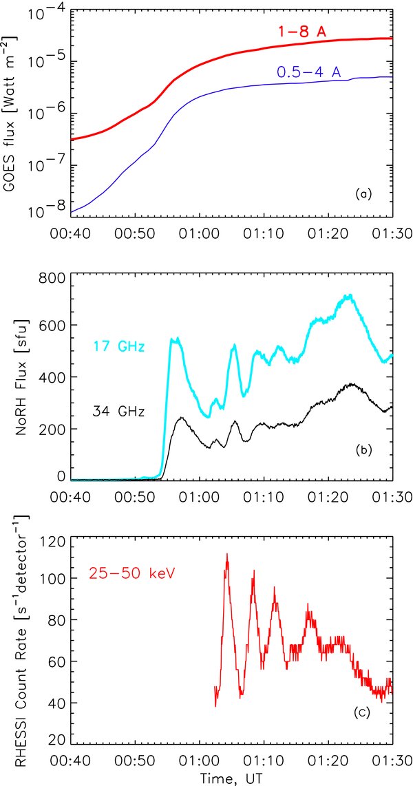
Figure 1. Light curves of the flare. (a) SXR in the GOES 1–8 Å (thick line) and 0.5–4 Å (thin line) channels; (b) NoRH fluxes integrated over the AR at 17 GHz (thick line), and 34 GHz (thin line); (c) HXR count rate measured in RHESSI 25–50 keV channel.
Download figure:
Standard image High-resolution image2.1. Pre-flare Hα and EUV Morphology of Active Region 10798
Evolution of AR structure prior to the flare was examined by Asai et al. (2009) and is shown in Figure 2. According to their study, AR NOAA 10798 emerged on 2005 August 18 and rapidly evolved. The arch-filament system can be seen in the Hα images on August 18 with a potential magnetic field connecting the sunspots of opposite polarity (Figure 2(a)). During 18–19 August the counterclockwise rotating motion of the sunspot pair was seen on magnetograms obtained by SOHO/MDI. We also found clockwise rotation of a preceding (positive polarity) sunspot after August 19. This rotation is particularly well seen during August 21. Due to this complex rotation motion, the Hα arch system was abruptly changed on August 21: clear oblique structure appeared (Figure 2(b)) and then a large filament evolved. The filament lies near the magnetic neutral line (NL) between the sunspots. This filament is seen as a bright J-shape structure on the EUV pre-flare images in Figure 3. The images were obtained about 20 minutes prior to the microwave flare onset with TRACE 171 Å, Figure 3(a), and SOHO/EIT 195 Å, Figure 3(b). The TRACE 171 Å spectral line is mainly sensitive to plasmas at a temperature around 1 MK (Fe ix) and SOHO/EIT 195 Å 1.5 MK (Fe xii). This J-shape structure consists of two parts: northern and southern, with no connectivity between them. The high spatial resolution (∼1'') of the TRACE images allows us to see more detail: multiple small loop system at the left of the filament's northern part. Superposed 17 GHz Nobeyama loops are shown by white contours on 0.04 and 0.1 levels of maximum brightness temperature, Tmaxb, at the flare onset time (1) 00:52 UT and (2) 00:53 UT. At the latter time, Tmaxb = 7.4 × 10⁵ K. The outer contour of loop FPs includes a corresponding part of the filament. RHESSI HXR sources observed at the time of flare 01:03:20 UT are shown by the dotted contour on plot (b). The southern HXR source coincides with the lower end of the J-shape structure. This bright EUV filament disappeared after the flare and the corresponding CME. There were no Hα and EUV observations during the microwave flare period.
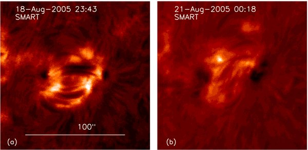
Figure 2. Evolution of the AR: Hα images obtained with SMART at Hida observatory. This figure was created on the basis of Figure 4 of Asai et al. (2009).
Download figure:
Standard image High-resolution image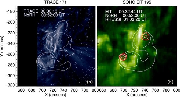
Figure 3. EUV images (gray scale) obtained with (a) TRACE 171 Å and (b) SOHO/EIT 195 Å prior to the flare. The 17 GHz loop is superimposed by white contour lines at levels 0.04 and 0.1 of Tmaxb at the time of flare onset. RHESSI HXR sources at levels 0.6, 0.7, 0.8, 0.95 of maximum counts are shown by dotted line on plot (b). Times are depicted on each plot. All images are rotated to the time 00:53:00 UT. The black part of the TRACE map is out of field of view.
Download figure:
Standard image High-resolution image2.2. Radio, Optical, and HXR Images of the Flare
Microwave flare morphology and its evolution are shown in Figure 4. Images of the source at 17 GHz (Stokes I) and 34 GHz, with black thin contours at levels 0.1, 0.3, 0.5, 0.7, 0.9 of maximum brightness temperature Tmaxb, are presented in the left and right columns, respectively. At the first emission peak time 00:56:34 UT, Tmaxb = 2.3 × 10⁷ K at 17 GHz and Tmaxb = 3.6 × 10⁶ K at 34 GHz. In Figure 4(a) the level 0.05 of Tmaxb is also presented. White dot-dashed lines show visible flaring loop axes. They were drawn using a spline approximation through the brightest points along the loop and used for measuring the apparent loop length. In the middle column, SOHO/MDI magnetograms (grayscale) are overlaid by black contours of polarization maps at 17 GHz (Stokes V) at 0.2, 0.4, 0.6, 0.8, 0.95 levels of the minimum brightness temperature Tminb. Only negative brightness temperatures were observed in polarization during the flare, with typical values of polarization degree of 30%. The magnetogram shows the negative (black color) and the positive (white color) magnetic structures. The white contour line shows the magnetic reversal line. All images are adjusted to the time of magnetogram 00:53:00 UT.
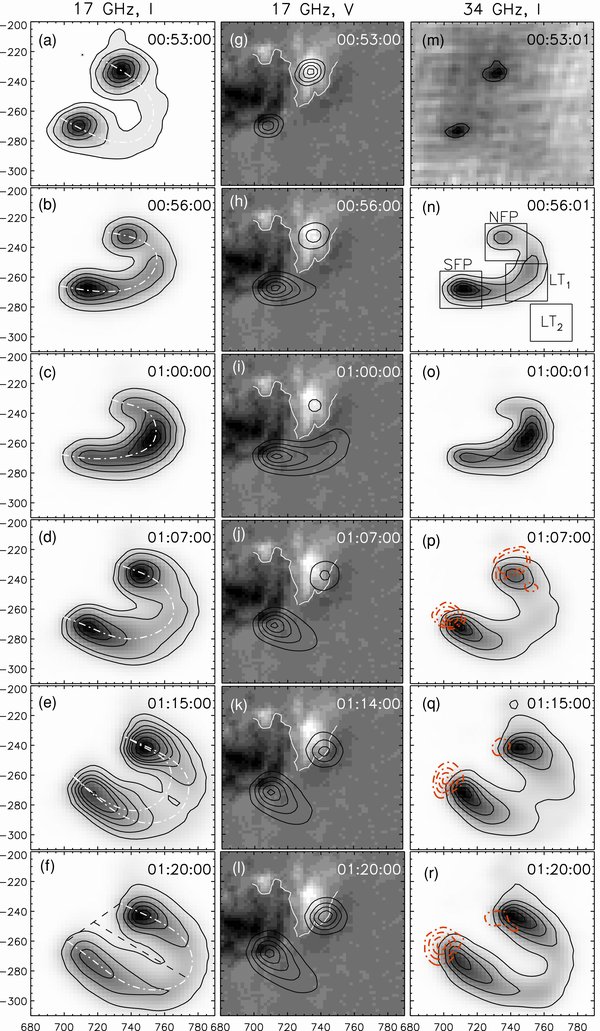
Figure 4. Evolution of the flare source morphology. Left column: NoRH images at 17 GHz, Stokes I. Contours correspond to 0.1, 0.3, 0.5, 0.7, 0.9 levels of Tmaxb. White dot-dashed lines show visible flaring loop axes, black dashed lines on (f) are loop span and height. Middle column: SOHO/MDI magnetogram (gray scale) taken at 00:53:00 UT overlaid by black contours of polarization images at 17 GHz (Stokes V) at 0.2, 0.4, 0.6, 0.8, 0.95 levels of the Tminb, all V values are negative. White contour line shows the magnetic reversal line. Right column: 34 GHz images (gray scale and thin black contours at the same levels as at 17 GH, I). On (p), (q), (r), HXR sources with energies 25–50 keV are superimposed by dot-dashed contour at 0.4, 0.6, 0.8, 0.95 levels of maximum count rates. Units of the X- and Y-axes are arcsec from the disk center. All images are rotated to the time of magnetogram.
Download figure:
Standard image High-resolution imageOn the rise phase of the flare, well-defined round-shaped FP sources of the loop are seen in intensity at both frequencies (Figures 4(a) and (m)). They correspond to the magnetic field of opposite polarity on the SOHO MDI magnetogram (Figure 4(g)). The magnetic field strength is Bmin ≈ 1300 G and Bmax ≈ +1800 G in the areas of the southern and northern polarization sources between levels 0.1 and 0.4 of Tminb.
Note that two FP sources have the same negative sign of circular polarization (Stokes V) at 17 GHz. This is quite unusual. Mostly we see positive Stokes V over the positive polarity of photospheric magnetic field, and negative Stokes V over the negative one. This happens in the case of optically thin gyrosynchrotron emission generated in magnetic loops located close to the solar disk center (Bastian et al. 1998). The polarization reversal in the case of our flaring loop happens for the northern source which is expected to have positive V. A well-known simple explanation of the reversal could be the optical thickness of the northern source. However, the spectral slope between 17 and 34 GHz derived from NoRH image data is always negative everywhere in the loop including the northern source. Therefore, the northern source is optically thin and this explanation of the reversal is not valid.
There are two other possible reasons for the polarization reversal, but both of them lack a robust observational basis to be proved. One of them is mode de-coupling for the emission coming from the northern source. This mechanism may work if the line of sight is perpendicular to the magnetic field in the northern source. The second reason may be a specific orientation of the flaring loop. The flaring loop under consideration is located far from the solar disk center and turned to the E-W direction. In this case, it may happen that it is oriented such that at its magnetic axes, the magnetic field vector everywhere in the loop has an obtuse angle with the direction of the line of site. Therefore, the sign of polarization should be the same everywhere in the loop as it is observed. Note that this interpretation also suffers from the lack of observational evidence.
On the maximum phase of the flare, an almost similar evolution was observed in intensity (Stokes I) at both frequencies, 17 GHz and 34 GHz: the entire loop structure was well seen during the whole of burst, but its orientation, length, and size changed with time. We used these images to measure the apparent loop length and LT height. In the period between 00:58:50 and 01:01:00 UT, the radio brightness gradually concentrated on the LT, FPs faded, and then the reverse process started. At about 01:15 UT, a new bright loop appeared at the higher altitude (Figure 4(e)). The top of this new loop is indicated as LT2. At the same time, the lower loop remained to be seen. After 01:23 UT, strong changes in the loop structure occurred. We do not show its further development.
RHESSI HXR maps at energies 25–50 keV are superimposed on plots of Figures 4(p), (q), (r) by the dot-dashed contour at 0.4, 0.6, 0.8, 0.95 levels of maximum count rates. We use the CLEAN method (Hurford et al. 2002) with natural weighting with grids 3–8 to construct HXR maps. In this way, RHESSI HXR maps have an FWHM spatial resolution of ≈10 arcsec.
From the figures, we can see that the centers of the two HXR sources approximately correspond to the 0.1 level of the Tmaxb 34 GHz loop. It should be mentioned that the northern HXR source may not be detected when it becomes weak, while the southern source is always present during the flare. The fainter HXR northern footpoint (NFP) is in good agreement with the stronger magnetic field here.
Note that at several time moments, the HXR emission is also detectable over the radio loop apex at levels 0.4–0.5 of the peak flux. These sources are clearly seen in Figure 5. This figure represents SOHO/EIT 195 Å images obtained at 02:32:44 UT, about 1 hr after the flare. Images show the post-flare arcade visible side. We superimposed the 17 GHz loop by white contour lines and RHESSI HXR sources by dotted lines for each temporal emission peak. Only those RHESSI maps that contain the HXR source near the radio loop apex were selected. Analysis of the RHESSI SXR images at energies 6–12 keV showed that the SXR loop system is located lower than the HXR coronal source at 01:12 and 01:19:40 UT.

Figure 5. EUV images (gray logarithmic scale) of post-flare arcade obtained with SOHO/EIT 195 Å at 02:32:44 UT. The 17 GHz loop is superimposed by white contour lines at levels 0.1, 0.3, 0.5, 0.7, 0.95 of Tmaxb at the time of each temporal peak. RHESSI HXR sources with energies 25–50 keV at levels 0.4, 0.7, 0.95 of maximum counts are shown by dotted lines on (b)–(f) obtained at the same time as NoRH images. Times are depicted on each plot. All images are rotated to the time 00:53:00 UT.
Download figure:
Standard image High-resolution imageFigure 5 shows that the flare was developing along the elongated arcade, from its northern part to southern. The radio loop together with HXR sources is following the direction and orientation of the EUV arcade.
2.3. Time Profiles
In Figures 6(a)–(c), we show the flux time profiles from the regions corresponding to different parts of the microwave loop. Flux densities are calculated from NoRH images by integration of brightness temperature over areas of the size 25'' × 25'', so that the area includes the changing location of FPs and LT during the flare process. The time resolution is 2 s. Dashed vertical lines are drawn to divide different emission peaks, which are numbered on the top of plot (a). It is interesting that the time profiles from both the southern footpoint (SFP) and the northern footpoint (NFP) consist of six emission peaks while there is only one (first) temporal peak in the LT1 source, which is much smoother. We limited LT1 flux evolution by 01:15 UT since after that the LT rises higher and reaches the level LT2, the northern leg occupies the area of LT1. Emission in the LT2 source gradually grows during peaks 4–6.
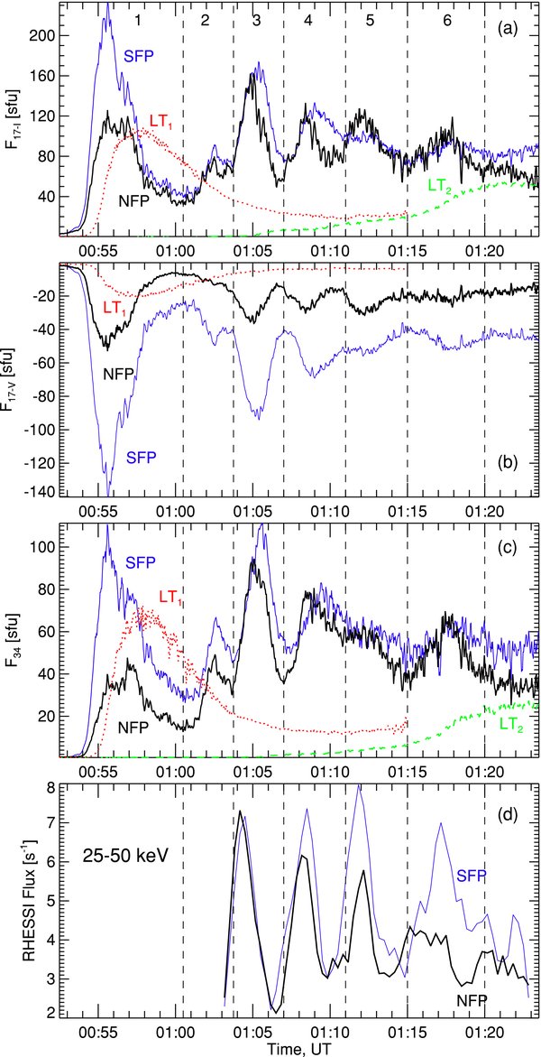
Figure 6. Time profiles measured with NoRH at (a) 17 GHz (Stokes I), (b) 17 GHz (Stokes V), (c) 34 GHz, and (d) with RHESSI at energies 25–50 keV. Flux densities from the southern FP (thin line), northern FP (thick line), LT1 (dotted line), and LT2 (dashed line) are obtained by integration over areas of the size 25'' × 25''. Locations of areas are shown in Figure 4(n).
Download figure:
Standard image High-resolution imageSurprisingly, SFP is brighter than NFP in microwave intensity at both frequencies 17 and 34 GHz during the first three peaks and it remains brighter in polarization during the entire flare. Taking into account that magnetic field is stronger in NFP, this fact contradicts the usual concept that the FP with the stronger magnetic field should have stronger radio emission and weaker X-ray emission. We suppose that the possible reason for this contradiction is a difference in the viewing angles for two FP sources; the viewing angle for the SFP source should be higher.
We can see time delays between NFP and SFP emission maxima, which are caused by kinetic effects inside the big loop. At the same time, we have found good temporal correlation between fluxes from two FPs on the smaller timescale (15 s) variations, which are in phase with peak-to-peak correspondence. These small-scale peaks are connected with the acceleration process inside each fine magnetic tube, which are not resolved with NoRH.
Figure 6(d) demonstrates time profiles of HXR emission in the 25–50 keV energy band for both NFP and SFP. RHESSI flux is calculated from RHESSI images by integration of counts over areas of the size 33'' × 33'' to improve the signal-to-noise ratio. The time resolution is 20 s. A comparison of microwave and HXR emission profiles shows one-to-one correspondence of their peaks with the delay of radio emission up to 1 minute.
2.4. Evolution of Spatial Characteristics
Figures 7(a) and (b) represent time profiles of the apparent loop length and height, respectively. The loop length is measured along the visible loop axis shown in Figure 4 between two foots on the level 0.1 of maximum Tb. This level corresponds to centers of HXR sources and, therefore, to the level of the Sun's chromosphere where the loop ends are anchored. The LT altitude is measured as a distance from the middle of the loop axis to the middle of the span between two FPs, as is shown in Figure 4(f).
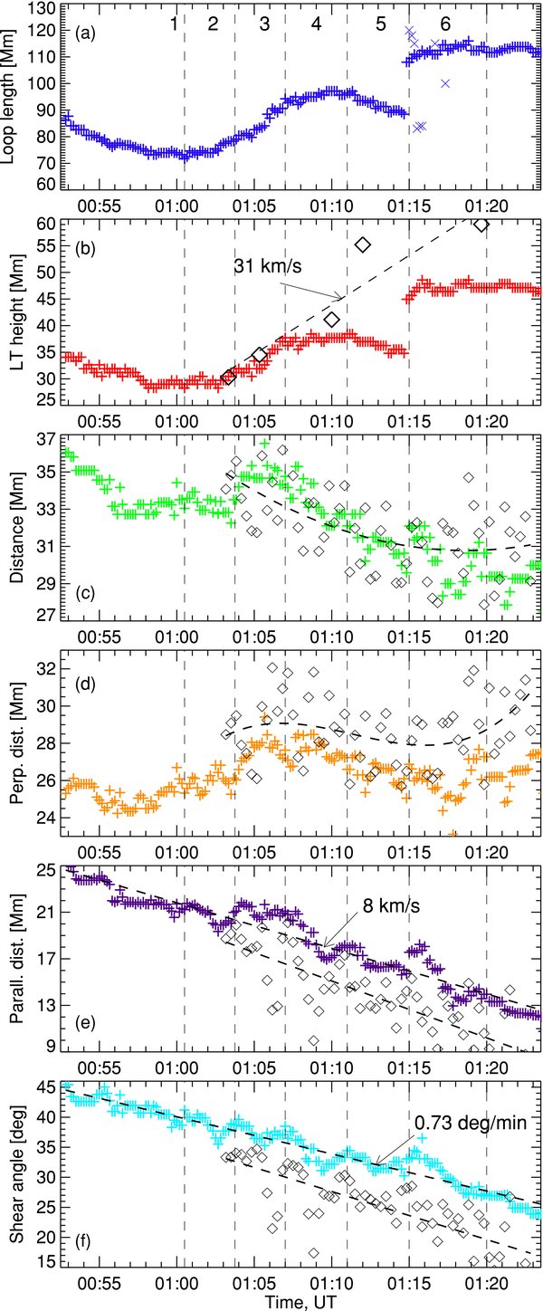
Figure 7. Time profiles for a number of quantities measured with NoRH at 17 GHz (crosses), and with RHESSI at energies 25–50 keV (diamonds): (a) apparent loop length and (b) altitude; (c) projected FP distance, with its components (d) perpendicular and (e) parallel to the magnetic inverse line; (f) shear angle. Dashed lines are (c, d) polynomial or (e, f) linear fitting of HXR time profiles.
Download figure:
Standard image High-resolution imageIt is clear that the brightness redistribution along the loop that occurred during the decay of the first peak and the rise period of the second peak influence the location of the 0.1 level of Tmaxb. This level is rising and descending together with the relocation of the brightness peak. To find out the time period of this influence we modeled the loop and changed the brightness of FPs and LT according to real time profiles shown in Figure 6(a). As a result, we found that brightness redistribution affects the location of the 0.1 level of Tmaxb between 00:56:30 UT and 01:02:00 UT, in the period when the ratio of fluxes from FP to LT FFP/FLT < 1 for both FPs.
Both parameters, the loop length and LT height, are decreasing at the rising phase (12% in the length and 8% in the altitude) and increasing during peak 3. During the fifth emission peak, we again observe the radio loop shrinkage in the length (12%) and height (8%) simultaneously with the formation of a new loop at higher altitude. The descending LT is observed for 4 minutes and it moves down with an average speed of 16 km s−1 at both periods. About 01:15 UT, a new bright loop appeared on the altitude 45 Mm, about 10 Mm higher than the previous loop. A detailed consideration of microwave images show that at the same time several other loops at different height levels with the lengths between 80 Mm and 120 Mm exist simultaneously. The average speed of the LT raising during the third to fifth emission peaks is 21 km s−1. The increase in the altitude is 38% and in the loop length is 28%. In Figure 7(b), we also show by diamonds the altitude of the HXR source observed over the radio loop (mentioned in Section 2.3). It is clearly seen that the HXR source altitude grows faster than the altitude of the microwave LT source. Its average speed is 31 km s−1.
The time profiles of the projected distance between two radio FPs (crosses) are given in Figure 7(c). It is measured between two ends of the loop axis on the level 0.1 of maximum Tb. The evolution of the perpendicular and parallel (to the magnetic NL) components of the FPs distance is shown in Figures 7(d) and (e), respectively. To calculate it we drew the simplified magnetic NL on the photosphere using the SOHO MDI magnetogram. The FP distance decreases during the rising phase with the speed v ≈ 16 km s−1. This contraction is caused by the decrease of both components, parallel and perpendicular. The apparent FP distance again falls into contraction after the second peak. But the last contraction is mostly due to unshearing motion.
Figure 7(f) represents the evolution of the flare shear angle. The shear angle is defined as the angle formed by the line connecting two conjugate FPs and the line perpendicular to the magnetic NL. Therefore, this is an analog of the parallel component of the FP distance. It was shown by Zhou & Ji (2009) that a flare shear is basically consistent with the magnetic shear computed from vector magnetograms and, therefore, is important for evaluating the magnetic nonpotentiality of a loop structure: the higher the angle is, the larger the magnetic nonpotentiality will be. The shear angle decreases from 45° to 25° monotonically in the course of the flare. The evolution of parameters at 34 GHz show the same tendencies, so we do not present it here.
In Figures 7(c)–(f), parameters measured with RHESSI at energies 25–50 keV are shown by diamonds. To determine the centroid positions of sources we use the center-of-mass method. Sometimes, there are two HXR sources associated with the NFP. We take them as one and use their weighted average position. We can see that polynomial approximation of time dependences for all four parameters obtained from HXRs have the same trends as time profiles obtained from microwaves. At the same time, vertical shifts between them are seen. To analyze the reason for these shifts we have measured the time evolution of distances between HXR and microwave sources for each FP. We found that the distance for the southern FP is systematically larger (3'') than that for the northern FP. This asymmetry gives a smaller parallel component of the FP distance and shearing angle and a larger perpendicular FP distance measured from HXRs as compared to microwaves.
An important issue here is the measurement accuracy. It is well known from the theory of interferometry (see, for example, Thomson et al. 1986) that the error of the determination of the contour level location or the brightness center position is significantly less than the interferometer beam size, which is about 10'' for 17 GHz. The accuracy increases significantly with the increasing signal-to-noise ratio. Because NoRH has high sensitivity, 5 × 10⁻³ sfu in flux density, the signal-to-noise ratio is very high during the flare (not less than 5). In this paper, we use detectors 3–7 to reconstruct RHESSI clean maps, in this way RHESSI HXR maps have an FWHM spatial resolution of about 10''. Even with detectors 3–7 RHESSI can determine source centroids to better than 1'' under the condition that both sources are well defined. However, due to the low signal-to-noise ratio, especially for the NFP, we have a significant dispersion of measured parameters. Standard deviation obtained from fitting is 2 Mm for distance and 3 7 for shearing angle. The corresponding standard errors for measurements with NoRH are 1 Mm and 14.
2.5. Footpoints and Loop Top Trajectories
In Figure 8, we drew the simplified magnetic NL on the photosphere (white line) and plotted FPs and LT source positions. Each color corresponds to different temporal emission peaks, which are depicted on the plot. The SOHO MDI magnetogram obtained at 00:50 UT is superimposed by contour lines, red for positive and blue for negative polarities. Contours show magnetic field on levels 150 G, 400 G, 600 G, 800 G for both positive and negative polarities. We can see that the NFP of the apparent bright loop moves predominantly along the magnetic NL in the southwest direction, and the position of the SFP is almost invariable. On the rising phase, the LT moves from south to north (black diamonds). Then, the entire loop was gradually stretching upward. After the fourth peak, the simultaneous descending of the brightest loop and the formation of a new microwave loop at higher altitude were observed.

Figure 8. FPs (crosses) and LT (diamonds) trajectories during the flare process obtained at 17 GHz (Stokes I) on an MDI magnetogram. The evolution in time is coded from dark to light colors. The SOHO MDI magnetogram is superimposed by contour lines, red for positive and blue for negative polarities. Simplified magnetic NL on the photosphere is shown by white line.
Download figure:
Standard image High-resolution image
3. DISCUSSION
Let us discuss the most interesting findings discovered from observations which are able to help in a reconstruction of the flare scenario.
3.1. Pre-flare Development
As we have shown in Section 2.1, due to the counterclockwise rotating motion of the sunspot pair and clockwise rotation of the leading sunspot prior to the flare, the Hα arch system evolved from the state with potential magnetic field to the sheared state with clear oblique magnetic loop structures. According to Figure 4, the overall NL has a reverse S shape, which is the other indirect evidence of a sheared magnetic field. In the past, a development of shear before flares was observed in the chromosphere from Hα (Tanaka & Nakagawa 1973 and others) and also in the photosphere in magnetograms (Hagyard et al. 1982 and others). It was considered as a signature of a storage of free energy in overlying corona via creation of nonpotential magnetic field. Existence of the magnetic shear, therefore, is an important indicator of initiation of a big solar flare.
It is clear from Figure 3 that the flare onset is associated with the J-shaped hot structure crossing the NL and seen in EUV: the southern and northern parts of the 17 GHz loop morphologically involve the corresponding part of J; the southern HXR source coincides with the southern end of the J-shape structure. Since the observed J-structure is bright in both TRACE 171 Å and SOHO/EIT 195 Å, its temperature must be around 1–1.5 MK. This kind of structure as well as S-shaped or sigmoidal configurations are often observed in SXR and EUV before and at the beginning of large flares/CME (Rust & Kumar 1996 and the subsequent investigators). They signify highly sheared magnetic flux ropes or so-called sheared core fields which harbor enhanced coronal heating (Moore et al. 2001). In the recent numerical simulation (Aulanier et al. 2010), a magnetic flux rope is heated through the slow photospheric bald-patch reconnection during the early formation of the sigmoid. Note here that for the AR under study, Asai et al. (2009) reported a new flux emergence around the magnetic NL and the formation of filaments at about 09:00 UT on August 21.
An eruption of sigmoidal, S-shaped, or J-shaped structures is believed to play an important role in large flare/CME events. This eruption may be initiated by some kind of instability (kink, torus) or by reconnection between two flux ropes (Moore et al. 2001; Kliem et al. 2004; Aulanier et al. 2010).
3.2. Unshearing Motion of Flare Loops
The motions of loops from a strongly sheared to a less sheared structure are often observed in Hα, HXR, and EUV (Masuda et al. 2001; Asai et al. 2003; Ji et al. 2006, 2007; Su et al. 2007; Liu et al. 2009). In this paper, such unshearing motion is also found from microwave observations for the first time. Indeed, as we reported in Section 2.4, during the flare process the shear angle of the loop steadily decreases. In the flare under study, this reduction is due to the NFP motion along the magnetic NL from the northern part to the southern part of the arcade. Therefore, reduction of flare shear has to be considered as an important component for the flare scenario/model.
3.3. Propagation of Flaring Process Along an Arcade of Loops
It is interesting that though we observe one single microwave loop during almost all of the flare process, the tracing of the loop's FPs and LT motion in this flare shows that the energy release and acceleration of electrons up to relativistic energies occur in sequence along the extensive arcade of loops. This arcade is well seen on Hα images prior to the flare and on EUV images after the flare. The bright well-visible radio loop as well as HXR FPs of the loop follows the direction and orientation of the EUV arcade, from its northern part to the southern. It means that successive emission peaks on the time profile occur in different parts of the arcade, not in the same magnetic loop. Particles are accelerated in a sequence of magnetic field lines along the arcade, and not in a single loop. A simultaneous existence of several LTs at different height levels at 01:15 UT (see Figures 4(e) and 7(a) and (b)) indicates that at least several loops become involved in the process.
3.4. Shrinkage and Stretching of the Flaring Loop
We have found the loop length contraction and LT descending motion with a speed v ≈ 16 km s−1 during the first peak of the microwave burst (see Figures 7(a) and (b)). In the second stage, after the first peak, since 01:02 UT the entire loop was gradually stretching upward with an average speed v ≈ 21 km s−1. After the fourth peak, the simultaneous descending of the brightest loop and formation of a new microwave loop at a higher altitude were observed.
A similar behavior was found by Li & Gan (2005) for the multicomponent time profile flare of 2002 August 24 observed with NoRH. They suppose that the expansion of the observed microwave loop is caused by a chromospheric evaporation induced by the intense energy injection during the first burst peak.
In the case of the flare 2005 August 22 we would not say that the expansion (stretching up) of the microwave loop is due to the high pressure caused by such an evaporation. We rather explain it by the appearance of new tiny flaring loops at higher and higher levels in the corona. This interpretation is clearly confirmed by the existence of several emission peaks (caused by several repeated injections) and by the observed changes of the loop FP locations (Figure 8).
The descending motion of the coronal source is typical for the initial phase of many other flares (Sui & Holman 2003; Sui et al. 2004; Li & Gan 2005, 2006; Ji et al. 2006, 2007; Veronig et al. 2006; Shen et al. 2008; Joshi et al. 2009; Liu et al. 2009). The derived shrinkage velocity of the radio loops agrees with the result of observations of LTs in HXR emission (8–45 km s−1; Sui & Holman 2003; Sui et al. 2004; Veronig et al. 2006) and in EUV observations (15 km s−1; Li & Gan 2006; Joshi et al. 2009).
The shrinkage of the loop length in the case of the 2005 August 22 flare is accompanied by converging motion of FPs both on the rising phase (first peak) and during the fifth peak. These two temporally associated phenomena were found in some other events (Ji et al. 2006, 2007; Liu et al. 2009).
There are several theoretical models that try to explain the considered two stages in the spatial development of flares. Most of them propose a very similar explanation for the second (expansion) stage of eruptive flares. The general idea is that during this stage a reconnection is occurring in a way similar to the reconnection in the standard model of large eruptive flares: new reconnected field lines appear higher and higher along a vertical current sheet. This process is followed by a gradual increase of the height of new flaring loops and increase of their FP separation transverse to the magnetic NL. The models by Somov (1986) and Bogachev et al. (2005) generalized this consideration taking into account the relaxation of sheared magnetic field near the NL. This allowed them to explain not only the transverse FP separation, but also a directed (unshearing) movement of FPs along the NL.
Our observations agree well with both above predictions. In the event under study the separation motion is found to occur during the second—third emission peaks, the separation reaches ≈2 Mm (Figure 7(d)). Since the loop is located far from the central meridian (heliographic coordinates S12°, W49°), projection effects there forbid precise measurements of distances along the view angle, i.e., perpendicular to the NL component of the FP distance. However, we can confidently measure the FP separation component parallel to the magnetic NL.
The dynamic shrinkage has various explanations. Within the magnetic reconnection process in solar flares it is expected that newly reconnected field lines relax by "shrinking" down to form a system of closed loops (Švestka et al. 1987; Lin et al. 1995; Forbes & Acton 1996; Lin 2004). In the numerical simulation of magnetic reconnection with heat conduction (Yokoyama & Shibata 1997, 1998; Chen et al. 1999), the downward jet collides with the line-tied magnetic loops, and a termination shock appears at the LT. The height of the bright loop decreases rapidly at the beginning until the LT reaches its minimum height. Thereafter it rises almost uniformly with time with its two FP separation. Depending on the model parameters, the LT height may show temporal variations, that is, sometimes it drops down against a rising background (Chen et al. 1999).
Veronig et al. (2006) give an interpretation of the LT altitude decrease in the frame of a collapsing magnetic trap model (Somov & Kosugi 1997; Karlický & Kosugi 2004) embedded in a standard two-dimensional reconnection flare model. Sui et al. (2004) suggested that the observed altitude decrease of the LT source might also be related to the change from slow X-point to fast Petscheck-type reconnection, which would not only increase the energy release rate but also push the lower bound of the current sheet downward. However, these scenarios cannot explain converging motion of FPs. Also, in two-dimensional models it is not possible to explain the observed propagation of the flaring process along an arcade and unshearing motions.
The explanation of the FPs converging simultaneously with the descending and unshearing motions of flaring loops is possible in the frame of three-dimensional models. In the "rainbow reconnection model" (Somov 1986), these phenomena are a consequence of three-dimensional magnetic reconnection at a separator in the corona. The separator is located above the photospheric NL like a rainbow above a river. During the first stage of the flare, the reconnection releases an excess of magnetic energy related to the magnetic tensions generated before a flare by the shear flows in the photosphere. The collapsing magnetic trap formed in the downflow after the reconnection at the separator explains the descending motion of the LT source. During the second phase, the ordinary reconnection process dominates, through which the energy release is described in terms of the standard model of large eruptive flares with increasing FP separation and upward motion of the LT source. The observed propagation of the flaring process along an arcade can also be understood in this unshearing process (Bogachev et al. 2005).
Note that the above model does not take into account a possible role of the activation of the J- or S-shaped filament located close to the NL. However, such a filament and a corresponding CME are important properties of the 2005 August 22 flare as well as of other powerful eruptive flares. According to the SOHO/LASCO CME on-line catalog5, the halo-type CME was first observed at 01:31 UT on the height h = 3.92 RSUN with the Large Angle Spectrometric Coronograph (LASCO) on board SOHO. Extrapolation shows that it started from 1 RSUN between 01:02 and 01:05 UT, i.e., just after the first temporal peak. This is strong evidence for the eruption of the filament observed in the preflare period.
Recently, many authors have exploited the idea that different kinds of instabilities or the loss of equilibrium can produce a dense plasma eruption and the accompanying flare process (Shibasaki 2001; Moore et al. 2001; Kliem et al. 2004; Tsap et al. 2008; Aulanier et al. 2010). An explanation of the first (shrinkage) and second (expansion) stages based on the idea of the erupting flux rope is considered by Ji et al. (2008). They assume that magnetic field lines in the arcade are distributed in such a way that the magnetic field that is close to the NL has a significant shear, and field lines are less sheared at longer distances from the NL. A flare is triggered by the magnetic reconnection in the middle of the sigmoid that produces a single long unstable twisted loop (flux rope) which moves upward. It first meets inner field lines with significant shear and then the outer magnetic field lines which are little sheared. Based on magnetic explosion conjecture (Hudson et al. 2000), Ji et al. (2007) showed that the release of magnetic energy will reduce magnetic shear and that the less-sheared arcade will have smaller height and span. The upward moving flux rope stretches the overlying magnetic field to form a vertical current sheet. In the second stage, the magnetic reconnection occurs in the current sheet at increasing altitude, producing two separating FPs/flare ribbons. We consider that this scenario is the most satisfying to our observations including pre-flare and second stages.
3.5. Two Stages in the Development of Microwave Emission
Two different stages can be clearly distinguished from the flux time profiles (Figure 6) in the development of microwave emission. The first stage corresponds to the first temporal peak on the microwave time profiles. This peak is well pronounced in emission at 17 and 34 GHz from both FPs and from the LT. The second stage corresponds to the period of the second to sixth peaks. In this stage, the temporal behaviors of the emission from the two FP regions and the LT region are completely different. Temporal peaks 2–6 are well pronounced in emission from the FP regions, their intensities are comparable with the intensity of peak 1. At the same time, the LT source emission is much weaker than it is during peak 1, looks very gradual, and does not show any emission peaks, except gradual increase during the sixth peak in the LT2 source.
Both gyrosynchrotron and free–free emission can contribute to the 17 and 34 GHz radio emission. However, our estimates show that gyrosynchrotron is much more efficient for this flare. To evaluate the contribution of the free–free radiation to the total flux we calculated the flux density of thermal radio emission from the whole radio loop using plasma temperature and emission measure obtained from GOES data. The evaluation shows that it is less than 1% at the first peak time and only 4% at 01:23 UT. Therefore, the contribution of the free–free radiation is very small. Also, the flare frequency spectra reconstructed with the Nobeyama Radio Polarimeter data show a typical gyrosynchrotron shape with the peak frequency fpeak ⩽ 10 GHz and negative slope over fpeak during the flare period. A calculation of the power-law spectral index α using flux densities at 17 and 34 GHz shown in Figures 6(a) and 6(c) indicates that this is true for all parts of the loop: α = −3 on the rise phase and then grows to α = −1 in the average for both the FPs and the LT. In the case of optically thin free–free emission one would expect a flat spectrum with α ≈ 0.
Model simulations making use of the non-stationary Fokker–Planck equation and calculation of gyrosynchrotron emission (Melnikov et al. 2002; Gorbikov & Melnikov 2007; Reznikova et al. 2009) show that the absence of secondary emission peaks in the LT is possible in the case of anisotropic injection of accelerated electrons into the loop predominantly along magnetic field lines. In this case, injected electrons pass quickly through the loop apex, generating emission of very small intensity, and then are reflected close to the ends of magnetic trap where they generate emission of much higher intensity due to the stronger magnetic field and high pitch angles. The observed picture can happen if the acceleration process occurs in a wide range of pitch angles in the first stage and then changes to the beam-like acceleration along the loop axes in the second stage of the flare.
We consider that the above-mentioned microwave emission properties in the second stage of the flare can be explained in the frame of the electron acceleration model in a collapsing magnetic field (Somov & Kosugi 1997; Bogachev & Somov 2005). The collapsing magnetic trap is a system of contracting magnetic field lines and the flowing plasma in the cusp magnetic field below the current sheet and above the relatively dense SXR flare loop with a quasi-stationary magnetic field. Somov & Kosugi (1997) and Bogachev & Somov (2005) have shown that the contracting local trap exists for 1–10 s and can serve as an efficient electron accelerator to relativistic energies via the first-order Fermi and betatron acceleration mechanisms.
The betatron electric field always increases the momentum perpendicular to the magnetic field. Therefore, it contradicts our conclusion about anisotropic injection of high-energy electrons along magnetic field lines in the second stage. The first-order Fermi acceleration gives an increase in the longitudinal particle momentum with decreasing separation between the magnetic mirrors of the local trap. Even if the initial particle distribution is isotropic, under the action of the Fermi acceleration the electron pitch angles decrease and the pitch-angle distribution is elongated along the large trap axis, which is in agreement with our conclusion. In the second stage of the flare, the Fermi acceleration may become more efficient than the betatron one due to, for example, a higher location of the current sheet over the flaring arcade (in other words, due to a longer local trap) and, therefore, result in a more beamed injection along the loop axes.
3.6. Relative Positions of HXR Coronal Source and Microwave Loop Apex
It is interesting that HXR coronal sources seen on several images (Figure 5) are located higher than the microwave loop apex and show faster upward motion. Above the SXR LT sources are usually referred to as Masuda sources. They are found in flares during the impulsive peak and were interpreted as evidence of magnetic reconnection above the SXR flaring loop (Masuda et al. 2001). However, in Masuda flares as well as in cases reported later (e.g., Veronig et al. 2006) the HXR LT source at higher photon energies is located at higher altitudes. According to the standard model, the reconnection progressively occurs at higher and higher altitude and, therefore, lower energy electrons are expected to situate at lower altitude where the reconnection process has occurred earlier. In the event under study, we observe the opposite situation: the microwave loop whose emission is generated by electrons of hundreds keV is located lower than the 25–50 keV HXR coronal source.
We consider that this situation again can be understood in the frame of the collapsing magnetic trap model. A large number of low-energy (tens of keV) electrons produced in the reconnection region and trapped locally in the collapsing field lines above the quasi-stationary magnetic loop can survive there for a fraction of second and generate the above loop HXR source. It is clear that at the same time a fraction of accelerated relativistic electrons can survive on the contracting field line of the large trap (flaring loop) for a much longer time than the lifetime of the local trap. They should generate microwave gyrosynchrotron emission even when the contracting line reaches its minimum height.
4. CONCLUSIONS
We have studied the spatial dynamics of the flaring loop in the large flare/CME event 2005 August 22. It has been found that the pre-flare morphology of the AR exhibits a strongly sheared arcade seen in Hα and accompanied with the J-shape filament bright in EUV. Two parts of the bright EUV filament spatially coincide with two 17 GHz FP sources at the time of the flare onset. During the whole burst, the entire loop structure was well seen at 17 and 34 GHz, but the loop's orientation, length, and size were changing with time. RHESSI observations showed two FP sources at 25–50 keV, as well as coronal sources that sometimes appeared over the radio loop apex.
The tracing of FPs and LT motion shows that energy release and high-energy electron acceleration occur in sequence along the extensive arcade that is well seen on Hα images prior to the flare and on EUV images after the flare. The motion of magnetic loops goes from the highly sheared to the less sheared state. The NFP of the apparent bright loop moves along the magnetic NL, and the position of SFP is almost invariable so that the shear angle of the loop steadily decreases during the flare process.
We have found that the loop length contracts and LT descends during the first emission peak accompanied by converging motion of FPs on the rising phase. Then, the entire loop gradually stretched upward. After the fourth peak the simultaneous descent of the brightest loop and formation of a new microwave loop at higher altitude were observed. The analysis of HXRs has shown a good correlation with results obtained from microwaves for the period of RHESSI observations.
We did not find one single flare model that could explain all observational findings. We consider the flare scenario similar to that proposed by Moore et al. (2001) and reported by Ji et al. (2008). The flare might be triggered by the activation of the J-shaped flux rope and its interaction with the highly sheared arcade. The upward moving flux rope stretches the overlying magnetic field to form a vertical current sheet. In the second stage, the magnetic reconnection occurs in the current sheet at increasing altitude, producing a rising LT and a stretching loop length. Additional evidence for such a scenario is SOHO/LASCO observations, which give an extrapolated rising start time of the filament just after the first temporal peak.
The revealed properties of time profiles of microwave emission confirm the existence of two stages in the development of the flare. In the first stage, which corresponds to the first temporal peak on microwave time profiles, the emission peaks are present simultaneously in the LT and FP regions at both frequencies, 17 and 34 GHz. In the second stage, after the first emission peak, repeated emission peaks are present only in the FP regions. We conclude that these two different stages are connected with differences in the acceleration process: in the first stage an injection of high-energy particles occurs in a wide range of pitch angles while in the second stage it changes to the beam-like acceleration along the loop axes and takes place over the flaring arcade. This situation can be explained in the frame of the collapsing magnetic trap (Somov & Kosugi 1997; Bogachev & Somov 2005), in which Fermi acceleration may become more efficient in the second stage of the flare. Note that the collapsing trap model is also able to explain the observed relative displacement of the microwave loop and the HXR coronal source, the latter being above the first.
The work was partly supported by RFBR-NSFC grant 08-02-92228, RFBR grants 07-02-01066 and 09-02-00624, and the Federal Programs "Scientific and Educational Manpower of Innovative Russia" No. 02.740.11.0246, No. P683/20.05.2010. The work of H. Ji was supported by NSFC 10833007. Authors are grateful to Dr. A. Asai and for providing us with the Hα data on the AR NOAA 10798 for use in this publication. We thank the anonymous referee for a number of useful comments.