


ABSTRACT
The logarithmic differential star count of the Two Micron All Sky Survey in Ks band can be well approximated by a single power-law luminosity function. With a fiducial Galactic structure, we measure the luminosity function for the entire Milky Way. The distribution of the power-law index is roughly isotropic and shows no obvious trend with the Galactic latitude. The value for the power-law index, the bright and the faint ends of the luminosity function are 1.85 ± 0.035, Ks = −7.86 ± 0.60 mag, and Ks = 6.88 ± 0.66 mag, respectively. Our result strongly supports the notion of a universal luminosity function in our Galaxy. We also find that the luminosity function of LMC/SMC is similar to that of the Milky Way.
Export citation and abstract BibTeX RIS
1. INTRODUCTION
Star count is a good way to investigate the structure of the Milky Way. Bahcall & Soneira (1980) proposed a two-component model, disk, and spheroid (halo), to interpret Galactic structure. However, Gilmore & Reid (1983) identified a third component, thick disk, which shares a similar density profile with the thin disk but consists of older stellar population. Either the two-component or the three-component model can fit star-count data without regarding other auxiliary parameters such as color, metallicity, space velocity, etc. Since then, many works have been carried out (see Karaali et al. 2004, and references therein), and now the three-component model is widely accepted. These studies are based on different observations with diversely limited/specific sky area, and the derived scale parameters are not always consistent. The reason is that the scale height and the local stellar number density normalization are tightly correlated (or anti-correlated to be exact). The smaller the scale height of the disk, the higher the local number density normalization (Chen et al. 2001; Siegel et al. 2002; Jurić et al. 2008). Moreover, the parameters of the Galactic structure might change along the Galactic coordinates (Du et al. 2006; Cabrera-Lavers et al. 2007; Bilir et al. 2006, 2008; Yaz et al. 2010). Therefore, a systematic study of a uniform and large area survey is necessary to pin down the parameters for the global structure of the Milky Way. For instance, the work carried out by Jurić et al. (2008) is a good example.
Not only the overall structure of the Milky Way, but also some specific features have been inspected, such as flares and warps. Based on the study of the Two Micron All Sky Survey (2MASS; Skrutskie et al. 2006) the effect of the warp is similar to that of gas/dust and the flare makes the scale height of the thick disk to increase with the galactocentric radius (see, e.g., Lopez-Corredoira et al. 2002; Momany et al. 2006; Cabrera-Lavers et al. 2007; Reylé et al. 2009). Recently, the halo has been carefully examined as well by using Sloan Digital Sky Survey data and indicates that two individual populations, inner and outer halos, might exist (Carollo et al. 2008).
In addition to structure, star count is also useful to study the stellar luminosity function of the Milky Way. For Galactic structure study, the common practice is to assume one luminosity function for the entire Milky Way. We may call this the universality hypothesis of the luminosity function (and thus the mass function). The star-count data are then used to find out the density profile. In general, there are two approaches for the luminosity function: empirical luminosity functions and stellar population synthesis. Empirically, one can use the observed luminosity function from the solar neighborhood to represent the disk population and that of globular clusters to represent the halo population. On the other hand, one may adopt a theoretical evolution of the Milky Way (by assuming an initial mass function and making use of our knowledge of stellar evolution) and use the resulting synthetic luminosity function. Both are widely used, but direct observations of NIR luminosity functions are scarce. If we reverse the procedure of the Galactic structure study, e.g., the star-count data are analyzed by using different luminosity functions with a fixed density profile, we can then assess the Galactic stellar luminosity function. For example, Bahcall et al. (1983) used optical data above 30° Galactic latitude to determine the power-law index of the luminosity function of the spheroid. However, it is not easy to separate the contributions from the individual smooth components of the optical wavebands star count to study the corresponding luminosity function. In contrast, the logarithmic differential star count (DSC) of 2MASS Ks band appears as a simple linear relation throughout the entire Milky Way. This suggests that a simple power-law luminosity function may suffice to explain the data. The coverage of 2MASS data provides a good opportunity to test the all sky universality hypothesis of the luminosity function.
In this work, we use the 2MASS point source catalog (2MASS PSC; Cutri et al. 2003; Skrutskie et al. 2006) to carry out the star count for the entire Milky Way and determine the Ks-band luminosity function for the whole sky. The model and its features are given in Section 2. Data and the analysis method are discussed in Section 3, and the results are presented in Section 4. Section 5 provides a summary and discussion.
2. THE MODEL
We define the DSC at a particular direction, ϕ(m), as the number of stars per unit apparent magnitude, m, within a certain solid angle of that direction (ΔΩ). It is a convolution of the local luminosity function ψ(M, r) with the stellar density profile, n(r), where r is the distance along the line of sight:
where the apparent magnitude m and the absolute magnitude M are related by the distance modulus

Here, A(r) is the extinction. In order to reproduce the simple linear relation shown in the logarithmic 2MASS Ks-band DSC, we adopt a single power-law luminosity function with cutoffs at the bright and faint ends:
Note that ψ(M) includes all luminosity classes. A single power-law luminosity function which includes both dwarfs and giants is not as far-fetched as it may sound. We are interested in near-infrared and in the relatively bright region of the luminosity function. Indeed some studies do indicate an approximate single power law in this region (see, e.g., Mamon & Soneira 1982; Eaton et al. 1984). Nevertheless, it is conceivable that some features of evolved stars may exist on top of the power-law luminosity function, for instance, the excess of red clump stars or other giants on the luminosity function which may be called "humps." Perhaps these humps would create an increase of stars on the DSC which may be called "bumps." However, in practice we do not find any identifiable bumps in our model, unless there is an overdensity region (such as the Galactic bulge, the Galactic inner bar, LMC, SMC, etc.) that exists somewhere along the line of sight and its number of stars dominates over the smooth background stellar distribution of the fiducial density profile (see below). There will be more on these issues later in the analysis method section and the summary and discussion section.
In Equation (3), ψ(M) is normalized to 1, and we assume that it is independent of r in accordance with the universality hypothesis of the luminosity function. The DSC of Equation (1) becomes
where rf and rb are the solutions of Equation (2) with M = Mf and Mb, respectively.
We adopt the galaxy model of Jurić et al. (2008) (see Table 1) for our density profile n(r). The model contains three major smooth components: thin disk, thick disk, and spheroidal halo (Bahcall & Soneira 1980; Gilmore & Reid 1983):

where R is the projection of the galactocentric distance on the Galactic plane, Z is the distance from the midplane, and n0 is the number density of star of the thin disk in the solar neighborhood. The thin disk D1 and thick disk D2 follow a double exponential law:
where (R☉, Z☉) is the location of the Sun, and hri and hzi are the scale lengths and scale heights of the disks (i = 1, 2; 1 for the thin disk and 2 for the thick disk). The spheroidal halo follows
where p is the power index and c is the flattening parameter. We adopted R☉ = 8 kpc (Reid 1993), Z☉ ≈ 0, and f1 = 1, f2 = 0.12, fH = 0.005. For other parameters, see Table 1.
Table 1. Fiducial Density Profile of Our Galaxy (Jurić et al. 2008)
| Component | Value | Uncertainty |
|---|---|---|
| Thin disk | ||
| Density law | Double exponential | |
| Scale height | 300 pc | 20% |
| Scale length | 2.6 kpc | 20% |
| Thick disk | ||
| Density law | Double exponential | |
| Scale height | 900 pc | 20% |
| Scale length | 3.6 kpc | 20% |
| Local normalization | 12% | 10% |
| Spheroid | ||
| Density law | Power law | |
| Power-law index | 2.8 | ≲0.2 |
| Flattening | 0.64 | ≲0.1 |
| Local normalization | 0.5% | 25% |
Download table as: ASCIITypeset image
For the extinction model, we adopt the new COBE/IRAS result (Chen et al. 1999) and convert it to Ks band by  (Schlegel et al. 1998).
Generally speaking, stellar density n(r) tends to a constant as r tends to zero (i.e., the solar neighborhood) and decreases exponentially when r is large. If 1 < γ < 2.5, the integrand of Equation (4) tends to zero when r tends to zero or infinity. Hence, if there exists a range of apparent magnitude, m, such that rf is small enough and rb is large enough, then the integral tends to a constant. The slope of the logarithmic DSC within this magnitude range is approximately 2(γ − 1)/5.
Figure 1 gives the logarithmic Ks-band DSC along with its slope. The logarithmic Ks-band DSC can be divided into bright, linear, and faint regions. Each region corresponds to the case of (a) rf < rb ≪ heff, (b) rf ≪ heff ≪ rb, and (c) heff ≪ rf < rb, respectively. The heff is the characteristic scale length of the density profile in a particular direction, e.g., toward the Galactic pole, heff is hz. The corresponding slopes of each region are 3/5, 2(γ − 1)/5, and fast drop-off. The transition from bright to linear is mainly determined by Mb, and that from linear to faint is mainly determined by Mf. We call them turning point and turnoff point, respectively. Although heff is also involved in determining the transitions, it only plays a relatively minor role. Since heff decreases with the Galactic latitude, the turning/turnoff point shifts to brighter apparent magnitude. The linear region moves to brighter apparent magnitude as well (Figure 2). The interstellar extinction does not alter the slope of the linear region, but it shifts the linear region to the dimmer magnitude (Figure 2), e.g., the dimmer turning point and the turnoff point. In addition, the turning point becomes sharper in the direction of the Galactic center (Figure 2).
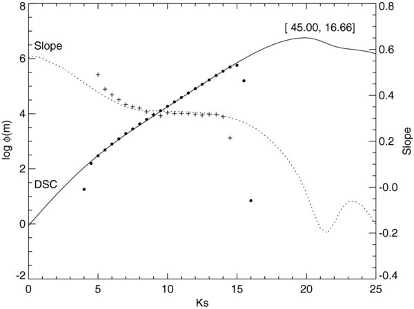
Figure 1. Logarithmic Ks-band differential star count (DSC) and its slope (i.e., power-law index). 2MASS data (circles) and its slope (pluses) are shown along with the model prediction (solid line and dashed line). The logarithmic Ks-band DSC can be divided into bright, linear, and faint regions. The corresponding slopes of each region are 0.6, 0.4(γ − 1), and fast drop-off. The direction of this example is [l, b] = [45, 16.66]. The fiducial Galactic structure is adopted from Jurić et al. (2008) (see Table 1). The turning point is around Ks = 8 mag and the turnoff point is around Ks = 20 mag, which is outside the 2MASS limiting magnitude. The quick drop at Ks = 5 mag of 2MASS data is due to the incompleteness of star detection for the relatively large photometric error from image saturation.
Download figure:
Standard image High-resolution image
Figure 2. Level-5 HTM logarithmic Ks-band DSC. Squares, circles and diamonds are 2MASS data, and lines are the model predictions. The solid line corresponds to the direction [l, b] = [308.85, 2.04]; the dot-dashed line corresponds to the same direction but with 3 times larger extinction; the dashed line corresponds to the high Galactic latitude [l, b] = [299.82, 82.40]; the dotted line corresponds to the direction of the Galactic center [l, b] = [9.39, 0.94]; and the number is shifted up by 1 order. The turning/turnoff point is dimmer for low latitude direction (solid line), and sharper toward the Galactic center (dotted line). The interstellar extinction does not alter the slope of the linear region, but it shifts the linear region to dimmer magnitude (dot-dashed line).
Download figure:
Standard image High-resolution image3. THE DATA AND ANALYSIS METHOD
3.1. The Data
Objects having a signal-to-noise ratio greater than 5 and detected in all J, H, and Ks bands are selected from the 2MASS PSC (Cutri et al. 2003). The limiting magnitude for the 2MASS Ks band is 14.3, which corresponds to 10 signal-to-noise ratio and has 99% completeness (see Table 1 in Skrutskie et al. 2006). The whole sky is divided into 8192 nodes according to the level-5 Hierarchical Triangular Mesh (HTM) (Kunszt et al. 2001) which samples the whole sky in roughly equal areas. The average distance of any neighboring two level-5 HTM nodes is about 2°. Our data bin size is Ks = 0.5 mag. The number of stars in each data bin within 1° radius of each level-5 HTM node is retrieved directly from the 2MASS online data service via the virtual observatory protocol (i.e., each level-5 HTM node covers π square degree). Only the Ks-band data are used in this study. Objects brighter than Ks = 5 mag are excluded in our analysis due to relatively large photometric error because of image saturation.
3.2. The Analysis Method
Maximum likelihood (Bienayme et al. 1987) is used to find the best-fit parameters of the luminosity function. We search for the minimum difference of 2MASS data for model prediction to obtain the best-fit parameters. Table 2 gives the magnitude ranges used in the fittings. The first two columns are the ranges for the Galactic latitude and longitude. The third column is the Ks magnitude range for maximum likelihood analysis. The magnitude ranges of all other areas that are not on the list are 5 < Ks < 14 mag. Only the first quarter of the Milky Way, [l, b] = [0°–180°, 0°–90°], is listed and the other three quarters mirror the first quarter.
Table 2. The Magnitude Ranges for Maximum Likelihood Analysis
| b (deg) | l (deg) | Ks (mag) |
|---|---|---|
| (0, 1) | (0, 60) | (5, 11) |
| (1, 2) | (0, 30) | (5, 11) |
| (1, 2) | (30, 60) | (5, 12) |
| (1, 2) | (60, 90) | (5, 13) |
| (2, 3) | (0, 35) | (5, 12) |
| (2, 3) | (35, 90) | (5, 13) |
| (3, 4) | (0, 30) | (5, 11) |
| (4, 5) | (0, 24) | (5, 11) |
| (4, 5) | (24, 30) | (5, 13) |
| (5, 8) | (0, 20) | (5, 11) |
| (8, 9) | (0, 15) | (5, 11) |
| (9,10) | (0, 15) | (5, 11) |
| (10,11) | (0, 9) | (5, 11) |
| (11,12) | (0, 7) | (5, 11) |
| (b ⩾ 60) | (0, 180) | (8, 14) |
Download table as: ASCIITypeset image
In the directions around the Galactic center, we avoid the shallower limiting magnitude around Ks = 11 mag and the bumps around 12 < Ks < 13 mag on the DSC. As mentioned in the model section, these bumps are due to the presence of the red clump stars of the Galactic bulge and the inner bar (see Figure 3 and Alves 2000; Hammersley et al. 2000). The overdensity of the bulge and bar dominates over the smooth background stellar distribution and enhances the red clump stars on the DSC. Except in the directions toward the Galactic center, LMC and SMC, no such bump on the DSC is observed.

Figure 3. Level-5 HTM logarithmic Ks-band DSC in the Galactic center direction. Circles (downshifted 1 order) and squares (upshifted 1 order) are 2MASS data. Lines denote model prediction. In our analysis, we avoid the red clump stars around Ks = 13 mag (square). The fitting tends to have a smaller power-law index, because of the upturn (around Ks = 9 to 10 mag) right after the turning point (around Ks = 8.5 mag) and the shallower limiting magnitude (around Ks = 11 mag).
Download figure:
Standard image High-resolution imageAt the high Galactic latitude regions (|b|>60°), we avoid the bright magnitude bins because of the large fluctuation in the number of stars. The fiducial Galactic structure we adopt is that of Jurić et al. (2008) (see Table 1).
First, the nodes around the Galactic center direction, [l, b] = [0° < l < 60° and 300° < l < 360°, − 10° < b < 10°] (516 nodes in total), have obvious turning points. We use these nodes to find the bright end of the luminosity function, Mb.
The high Galactic latitude nodes were used to find the faint end of the luminosity function, Mf. In order to check whether the turnoff point is within the 2MASS Ks-band limiting magnitude, we also include the Chandra Deep Field South (CDFS) data (Groenewegen et al. 2002; Girardi et al. 2005) to examine the faint end of the luminosity function. The Ks band of CDFS data covers only 0.0928 deg2 at [l, b] = [220 0, − 539]. We normalized the CDFS data to π deg2 field of view and combined with the closest node of our sample ([l, b] = [2216, − 535]). Figure 4 shows that the turnoff point of the 2MASS+CDFS data is outside the 2MASS Ks-band limiting magnitude. The best-fit value of the faint end of the luminosity function from the combined data is Ks = 7.5 mag. With this value, the downtrend of turnoff point begins around Ks = 14 mag in the high Galactic latitude direction. Therefore, the downtrend of the turnoff point of the high Galactic latitude nodes, |b|>60° (1280 nodes in total), was used to determine the faint end of the luminosity function, Mf.
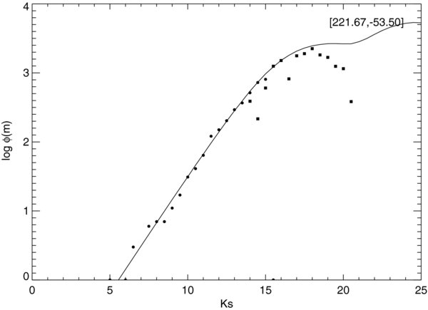
Figure 4. Logarithmic Ks-band DSC of 2MASS and CDFS data. Circles and squares denote 2MASS and CDFS data, respectively. The 0.0928 deg2 CDFS data are normalized to our π deg2 field of view. The solid line represents the model prediction.
Download figure:
Standard image High-resolution imageAfter the bright/faint ends of the luminosity function are fixed, the best-fit power-law index of the luminosity function, γ, is searched for every node in the entire sky. The parameters of the space we search are [γ, Mb, Mf] = [1.6 < γ < 2.2, − 9.5 < Mb < −5.5, 5.5 < Mf < 9.9] with the grid size [0.01, 0.5, 0.5]. Figure 5 shows some examples of our logarithmic DSC fitting.
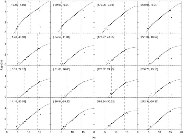
Figure 5. Examples of our DSC fitting. Circle is 2MASS data and line is the model prediction. The direction [l, b] is marked on each panel.
Download figure:
Standard image High-resolution image4. RESULTS
The distributions of the bright/faint ends of the luminosity function are shown in Figure 6. The mean values of the bright and faint ends are Ks = −7.86 ± 0.60 and Ks = 6.88 ± 0.66 mag, respectively, with uncertainty 1σ from the normal distribution. The faint end of the luminosity function is comparable with the result of 2MASS+CDFS data, Ks = 7.5 mag (with 0.5 mag searching grid). Since the downtrend of turnoff point at the high Galactic latitude is marginal around the limiting magnitude, it is easily biased by the fluctuation of the number of stars. Perhaps this is the reason for the tail at Ks = 9.5 mag of the distribution of the faint end. We expect that the tail will diminish if the limiting magnitude can be pushed 1 or 2 mag deeper.

Figure 6. Distribution of the bright/faint ends of the luminosity function from the 2MASS DSC. The bright end, Mb, is determined from the nodes around the Galactic center ([l, b] = [0° < l < 60° and 300° < l < 360°, − 10° < b < 10°], 516 nodes in total), and the faint end, Mf, from high galactic latitude data (|b|>60°, 1280 nodes in total).
Download figure:
Standard image High-resolution imageThe distribution of the power-law index of the luminosity function is shown in Figure 7. The mean value of all sky (8192 nodes), Galactic plane (|b| < 10°, 1592 nodes), low (|b| < 30°, 4264 nodes), medium (30° < |b| < 60°, 2648 nodes), and high Galactic latitude (|b|>60°, 1280 nodes) are 1.85 ± 0.04, 1.82 ± 0.02, 1.84 ± 0.03, 1.85 ± 0.03, and 1.86 ± 0.04, respectively (see Table 3). (Note that "low latitude" includes "Galactic plane.") Although the mean value increases slightly along the Galactic latitude, the differences are all within 1σ deviation. There is no correlation between the power-law index and the Galactic latitude. Moreover, the power-law index is roughly isotropic for the entire Milky Way (see Figure 8).
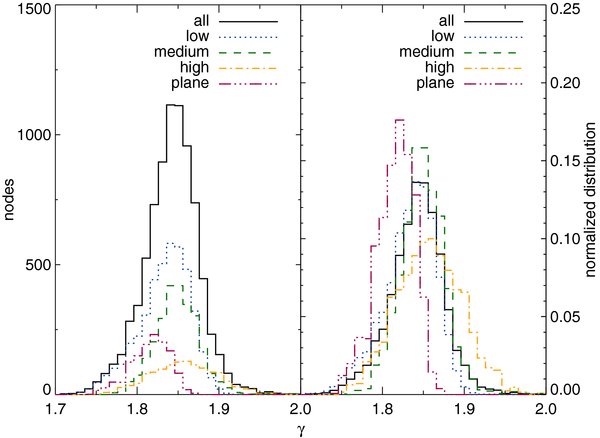
Figure 7. Distribution of the power-law index of the luminosity function. The solid, dotted, dash, dot-dashed, and dotted-dotted-dash lines represent the whole sky, low, medium, high latitude, and the Galactic plane, respectively (see the text or Table 3 for their corresponding latitude ranges). The distributions in the right panel are all normalized to one.
Download figure:
Standard image High-resolution image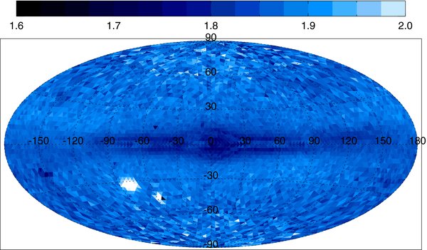
Figure 8. Whole sky power-law index plot. It is roughly isotropic. The two bright spots in the southern hemisphere are LMC and SMC.
Download figure:
Standard image High-resolution imageTable 3. The Power-law Index of the Luminosity Function
| Area | Index | Number of Nodes |
|---|---|---|
| All sky | 1.85 ± 0.04 | 8192 |
| |b| < 10° | 1.82 ± 0.02 | 1592 |
| |b| < 30° | 1.84 ± 0.03 | 4264 |
| 30° < |b| < 60° | 1.85 ± 0.03 | 2648 |
| |b|>60° | 1.86 ± 0.04 | 1280 |
Download table as: ASCIITypeset image
Several factors may affect the smaller power-law index in the direction of the Galactic center. Due to the shallower limiting magnitude, the linear region of the logarithmic DSC covers only a small magnitude range. The incompleteness of star detection at the faint end of the DSC causes the luminosity function to become flatter. The bump right after the turning point is not well fitted by the model. Perhaps a more sophisticated model for the Galactic center direction is needed, e.g., a more accurate extinction model or another Galactic center component of the density profile (see Figure 3).
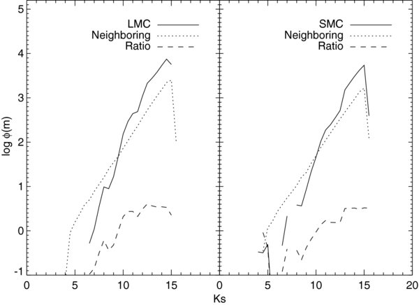
In the LMC and SMC directions, we see an obvious increase or jump in the logarithmic DSC around Ks = 10.5 and Ks = 11 mag, respectively (see Figure 9). Such a jump is due to the clumpy stellar distribution of LMC and SMC. For magnitudes smaller than the jump, stars come solely from the Milky Way. For larger magnitudes, stars from LMC and SMC are seen in addition to the foreground stars from the Milky Way. The jump makes the fitting have a larger power-law index (a steeper luminosity function) for the nodes associated with these two satellite galaxies. Therefore, the power-law indices in these two directions are not reliable. In any case, the jump of LMC/SMC data represents the bright end of the LMC/SMC luminosity function. When we take 48.1 kpc/60.6 kpc as the distances of LMC/SMC (Macri et al. 2006; Hilditch et al. 2005) to covert the jump to the bright end of the LMC/SMC luminosity function, we obtain Ks = −7.91/Ks = −7.91 mag. This is close to that of the Milky Way, Ks = −7.86 ± 0.60. Assuming that the foreground stars of the Milky Way can be approximated by their surroundings, we subtract the foreground and obtain the star content of LMC and SMC. Since the bright ends of LMC and SMC DSC are fainter than Ks = 10.5 mag, it is difficult to obtain a reliable power-law index. Instead, we work out the ratio of LMC/SMC to their surroundings. The jumps become more obvious in these ratios (dashed line in Figure 9). Beyond the jumps, the ratio is roughly constant which implies that the DSC of LMC/SMC and their surroundings, e.g., the stars of our Galaxy, have a similar power-law index.
Figure 9. Logarithmic Ks-band DSC within 5° radius of LMC (left) and that within 3° radius of SMC (right). The neighboring areas are from 7° to 15° and 5° to 10° rings of LMC and SMC, respectively. The dotted line in both panels is the corresponding neighboring DSC. The solid line is the LMC/SMC DSC in which the foreground stars of the Milky Way is removed (assuming that the foreground stars can be approximated by the neighboring DSC). Both LMC/SMC and the neighboring DSC are average to π deg2 field of view. The dashed line is the ratio of the LMC/SMC DSC to their neighboring DSC. The jump in logarithmic LMC and SMC DSC are ∼10.5 and 11.0 Ks magnitudes, respectively. The ratio is roughly constant after the jump.
Download figure:
Standard image High-resolution image
5. SUMMARY AND DISCUSSION
The logarithmic 2MASS Ks-band DSC can be well approximated by a single power-law luminosity function. This provides a good opportunity to examine the luminosity function for the entire Milky Way. We aim at finding the global behavior of the Milky Way luminosity function. We do not intend to identify any specific detail features neither on the luminosity function, such as red hump, horizontal branch, and globular cluster dip, etc., nor on the Galactic structure, such as flare, warp, 3 kpc bar, and center bulge, etc. None of these features affect the general shape of the logarithmic Ks band DSC predicted by our model.
We adopt a single power-law luminosity function with abrupt bright and faint-end cutoff. The analysis of these parameters of our luminosity function comprises three steps.
- 1.The bright end of the luminosity function is obtained from directions around the Galactic center ([l, b] = 0° < l < 60° and 300° < l < 360°, − 10° < b < 10°]), and the result is Ks = −7.86 ± 0.60 mag.
- 2.The faint end of the luminosity function is obtained from the high Galactic latitude areas (|b|>60°), and the result is Ks = 6.88 ± 0.66 mag.
- 3.The power-law index of the luminosity function is measured with the bright and faint ends found in steps 1 and 2. The whole sky power-law index is roughly isotropic and the value is 1.85 ± 0.04.
A detailed look at the power-law index distribution shows that there is a slight increase in the power-law index at the high Galactic latitude but it is not significant (see Table 3). The power-law index is larger in the directions of LMC and SMC and smaller in the Galactic center direction. On the Galactic plane, the power-law index is slightly smaller. Other than these, we do not see any particular patterns on the whole sky map of the power-law index.
Most if not all the luminosity functions used in star-count studies in optical and NIR bands can be approximated by a broken power law, in which two power laws (the bright part and the faint part) are joined by a break point (Mamon & Soneira 1982; Eaton et al. 1984; Bahcall 1986). However, the 2MASS data can be well fitted by a single power-law luminosity function in our analysis. One possible explanation is that the 2MASS data only represent the bright part power law, and the faint part, if it exists, is not observed because of the shallow limiting magnitude of 2MASS. For instance, information on the luminosity function fainter than Ks = 6.88 mag is not available from 2MASS data. Consequently, we cannot rule out that the Ks-band luminosity function is a broken power law, but our analysis showed that the break point, if it exists, cannot be brighter than the faint end of our luminosity function, Ks = 6.88 ± 0.66 mag.
In order to know how the determination for luminosity function is affected by the uncertainty and the bias-correction of the fiducial Galactic model (see Table 10 in Jurić et al. 2008), we have tested our results for different scale lengths and scale heights. We found that a 20% uncertainty and the bias-correction of the fiducial Galactic model will not affect our conclusion.
We also find that the ratio of the DSC of LMC/SMC to the Milky Way is roughly constant which indicates that the DSC of our Galaxy, LMC, and SMC may have a similar power-law index. Moreover, their bright ends of the luminosity function are close as well. This implies that the Milky Way, LMC, and SMC may have a similar luminosity function.
To summarize, our analysis strongly supports the universality hypothesis of the luminosity function in our Galaxy (and thus the mass function). In addition, the luminosity function of LMC/SMC may be similar to that of our Galaxy. Now we have observational confirmation of the hypothesis, but the question "why it is so" is still unanswered.
Finally, in 2MASS data we find that only the Ks band shows a considerable linear region on the logarithmic DSC (J, H, and optical bands do not). Interestingly, the Arkari 9 μm data (Ishihara et al. 2010) also show such a significant linear region. Is this a coincidence or a universal property of longer wavelength bands?
We acknowledge the use of the Two Micron All Sky Survey Point Source Catalog (2MASS PSC) and Chandra Deep Field South (CDFS). We thank the Japanese Virtual Observatory for helping us with online data retrieval. We also thank the referee whose comments helped us to improve the paper significantly. This work is supported in part by the National Science Council, Taiwan, under the grants NSC-96-2112-M-008-014-MY3, NSC-98-2923-M-008-001-MY3, and NSC-99-2112-M-008-015-MY3.