


ABSTRACT
The 18O(p, α)15N reaction is of primary importance to pin down the uncertainties, due to nuclear physics input, affecting present-day models of asymptotic giant branch stars. Its reaction rate can modify both fluorine nucleosynthesis inside such stars and oxygen and nitrogen isotopic ratios, which allow one to constrain the proposed astrophysical scenarios. Thus, an indirect measurement of the low-energy region of the 18O(p, α)15N reaction has been performed to access, for the first time, the range of relevance for astrophysical application. In particular, a full, high-accuracy spectroscopic study of the 20 and 90 keV resonances has been performed and the strengths deduced to evaluate the reaction rate and the consequences for astrophysics.
Export citation and abstract BibTeX RIS
1. INTRODUCTION
1.1. Astrophysical Background
Asymptotic giant branch (AGB) stars play a major role in nuclear astrophysics as the site for synthesis of heavy elements, which occurs through neutron capture reactions and beta decay along the line of stability, the so-called s-process (Herwig 2005; Busso et al. 1999; Lugaro et al. 2004). Spectroscopic observations show that, in these stars, fluorine is significantly enhanced compared with its solar abundance (Jorissen et al. 1992). Because 19F is produced in the He intershell and then dredged up to the surface together with s-process elements, its abundance can be used to constrain AGB models as it is sensitive to the efficiency of the dredge-up and to the physical conditions in the deep layers of the stars (Lugaro et al. 2004). When the abundances predicted by the current models are compared with the observed ones, an unacceptable discrepancy shows up even when model parameters are varied in a reasonable range (Lugaro et al. 2004). It has been pointed out that extra-mixing processes, such as the cool bottom process (Nollett et al. 2003), may help to provide predictions in better agreement with observations (Lugaro et al. 2004). An alternative view claims that the disagreement can be alleviated, at least partially, if current observed abundances are biased by systematic errors (blending of the spectroscopic lines not accounted for (Abia et al. 2009)). Other observables that turn out to be very sensitive to the mixing processes are the isotopic ratios of the abundances of some CNO isotopes, such as 18O, 17O, 15N, and 13C to the most abundant ones, namely 16O, 14N, and 12C (Nollett et al. 2003). These isotopic ratios are determined with good accuracy from the analysis of meteorite grains, that is, tiny intruders formed in the cold, outermost layers of AGB stars, which keep the fingerprints of the nucleosynthesis processes and of the mixing mechanisms taking place inside these stars. In particular, it turns out that it is hard to explain the exceedingly small 14N/15N values, which are even smaller than the solar ratio, with AGB stars in any evolutionary model that assumes solar elemental abundance as the initial condition. This is because any proposed approach tends to burn 15N, thus further increasing the 14N/15N ratio (Nollett et al. 2003). A possible way to explain the 19F abundance in AGB star envelopes and isotopic ratios in meteorite grains without introducing additional hypotheses might be provided by nuclear physics, more precisely by the 18O(p, α)15N reaction. Indeed, this reaction represents the main 15N production channel, both in the intershell region and at the bottom of the convective envelope (Nollett et al. 2003; Lugaro et al. 2004). During the thermal pulse, 15N is burnt to 19F via the 15N(α,γ)19F reaction. Thus, a larger 18O(p, α)15N reaction rate would lead to an increase of the 19F supply as well as to an enrichment of 15N in the stellar surface. Moreover, a 15N enrichment can be determined by 18O p-induced burning at the bottom of the convective envelope and by the mixing processes bringing the processed material to outer layers (Huss et al. 1997).
Peculiar 18O and 19F abundances have also been observed in post-AGB stars, in particular in the so-called R Coronae Borealis (RCB) stars (Clayton et al. 2007; Pandey et al. 2008). Indeed, these stars show 16O/18O ≲ 1, as measured in vibration–rotation CO spectra, that is hundreds of times smaller than the standard Galactic values. Two scenarios have been proposed to explain the origin of RCB stars, namely the "final flash" model (FF) and the "double degenerate" (DD) model. In the former, a final He-shell flash in a post-AGB star creates a H-poor supergiant while in the latter the luminous star is formed by accreting material from a He white dwarf onto a CO white dwarf in a close binary system. It has been found (Clayton et al. 2007) that only the DD scenario can provide a qualitative account of 18O and 19F abundance enhancements, provided that H-rich material, from the white-dwarf thin envelope, is admixed. In fact, through the 18O(p, α)15N(p, α)12C chain the 16O/18O and the C/N ratios are brought to the observed values, thus reversing the effect of excessive He burning, while fluorine is produced by p-radiative captures on 18O. Again, a revised 18O(p, α)15N reaction rate can provide a clue to better understand these rare and exotic systems.
1.2. Previous Studies
The low energy cross section of the 18O(p, α)15N reaction has been the subject of several experimental investigations (Mak et al. 1978; Lorentz-Wirzba et al. 1979) and many features are known from spectroscopic studies (Yagi et al. 1962; Champagne & M. Pitt 1986; Wiescher et al. 1980; Schmidt & Duhm 1970; Wiescher & Kettner 1982). These studied were triggered by the need to extend the knowledge of the cross section down to very low energies, looking for unknown resonances that may have interest both for astrophysics and 19F spectroscopy. For instance, the exceedingly strong 144 keV resonance was identified in Lorentz-Wirzba et al. (1979), thus spoiling any prediction in the previous paper (Mak et al. 1978). In the same way, other low-energy resonances might drastically change the trend of the cross section at sub-Coulomb energies as well as subthreshold resonances, especially in the case of broad ones (Rolfs & Rodney 1988). Despite their importance, the properties of the resonances lying below 70 keV are known only through indirect spectroscopic studies as the cross section drops exponentially. For instance, the cross section at 20 keV is a factor of about 1011 smaller than the one at 70 keV because of the Coulomb barrier penetration factor, thus making any attempt of measuring the cross section at such energies unfruitful, at least with the present-day facilities. It is worth noting that 20 keV is well within the range of center-of-mass (c.m.) energies of interest for astrophysical applications, namely the Gamow window (Rolfs & Rodney 1988), extending from 17 keV to 53 keV for T = 2 107 K, which is a typical temperature characterizing burning processes at the bottom of the convective envelope (Lugaro et al. 2004). Even though several studies have focused on the low energy region (Lorentz-Wirzba et al. 1979; Champagne & M. Pitt 1986; Wiescher & Kettner 1982), nevertheless the reaction rate for the process is affected by a considerable uncertainty (Angulo et al. 1999). Indeed, below 1 MeV nine resonances occur, but the reaction rate is essentially determined by the 20 keV, 144 keV, and the 656 keV resonances (Angulo et al. 1999). Only the contribution of the 144 keV resonance is soundly established. With regard to the 20 keV resonance, its strength is known only from spectroscopic measurements performed through the transfer reaction 18O(3He, d)19F (Champagne & M. Pitt 1986) and the direct capture reaction 18O(p, γ)19F (Wiescher et al. 1980). Though these studies represent an important way to estimate the strength of such low-laying resonance, the use of spectroscopic factors can severely spoil the accuracy of the results as they depend on the set of optical model parameters chosen to fit the data. In addition, the poor knowledge of the resonance energy makes a major contribution to the uncertainty of the reaction rate. To summarize, the most recent compilation, NACRE (Angulo et al. 1999), provides the resonance-strength recommended value ωγ = 6+17−5 10−19 eV, where the wide range reflects both the large uncertainties that affect the experimental values and the scatter of the data from different measurements. In the same way, the 656 keV resonance gives a sizable contribution to the low energy region for its total width turns out to be quite large (100 keV, Yagi et al. 1962; or 342 keV, Lorentz-Wirzba et al. 1979). Though it lies at energies where the cross section measurement is within the reach of available nuclear physics laboratories, its width and resonance energy are not well determined. We have already shown (La Cognata et al. 2008b) the large disagreement (up to a factor three) among different estimates of the resonance width, while a smaller difference can be found in measured resonance energies (644 keV, Yagi et al. 1962; or 658 keV, Lorentz-Wirzba et al. 1979). These uncertainties propagate to the resonance strength, whose recommended value is ωγ = (5.5 ± 1.0) 103 eV, coming from the average of the values from Yagi et al. (1962) and Lorentz-Wirzba et al. (1979; see Angulo et al. 1999 for a more detailed discussion). A poor knowledge of the cross section behavior also comes from the lack of information on the spin and parity of the 8.084 MeV level in 19F (corresponding to a 90 keV resonance in the 18O(p, α)15N cross section).
1.3. Electron Screening. The Need for Indirect Methods
It is worth stressing that, even if the cross section measurement for 18O(p, α)15N is extended down to astrophysical energies, electron screening effects would inhibit a determination of the cross section for the 18O−p interaction (Assenbaum et al. 1987; Fiorentini et al. 1995; Strieder et al. 2001). The presence of atomic electrons produces an enhancement of the cross section when the c.m. energy approaches zero, which is not related to the nuclear interaction (e.g., subthreshold resonances) in the 18O−p channel. For instance, in the case of the 18O(p, α)15N reaction an increase of the cross section by a factor of ∼2.4 is expected at 20 keV (Assenbaum et al. 1987). Since the interacting particles are in the form of neutral atoms, molecules or ions in the laboratory, electron clouds partially shield nuclear charges, thus reducing the Coulomb suppression effect. The enhancement factor fenh(E) (Assenbaum et al. 1987; Fiorentini et al. 1995; Strieder et al. 2001) is given by
where σs(E) and σb(E) are the screened and bare-nucleus cross sections, namely the cross section the particles would have if stripped of all the surrounding electrons, η is the Sommerfeld parameter, and Ue is the electron screening potential. Clearly, the enhancement factor depends only on a single parameter, Ue, which in principle can be evaluated according to atomic physics theories. The bare-nucleus cross section can be obtained accordingly, dividing out the enhancement factor; this step is necessary for astrophysical application since nuclei in stellar plasma are fully stripped of their electrons because of the high temperatures in the inner layers. Indeed, a different enhancement factor is introduced in stellar environments to account for plasma effects (Rolfs & Rodney 1988). It turns out that current atomic models cannot provide Ue values, for a broad range of reactions, which satisfactorily agree with experimental electron screening potentials Ue (La Cognata et al. 2005a and reference therein). This can make the bare-nucleus cross section σb(E) obtained by correction highly inaccurate, especially at the lowest energies where the enhancement can be as much as a factor two or larger. Therefore, even in those few cases in which the measurement has been performed down to astrophysical energies, extrapolation is required to evaluate the bare-nucleus reaction cross section. To achieve a more accurate extrapolated trend, the astrophysical S(E)-factor is used in place of the cross section (Rolfs & Rodney 1988):

where the inverse Gamow factor exp(2πη) is introduced to compensate the steep drop of the cross section due to the Coulomb nuclear repulsion, so as to get a smoother function. Even so, extrapolation can miss the contribution of unknown levels, also below the reaction threshold, especially when no theoretical models are used to predict the behavior of the cross section. Again, large uncertainties can be introduced into the astrophysical predictions due to inaccurate extrapolated cross sections, which do not match the unknown, true ones. For these reasons, the so-called indirect methods have been introduced, aiming at accessing the low energy cross section with no need of extrapolations.
2. THE THM APPROACH
The indirect label is used to refer to those techniques that allow one to deduce the S(E)-factor of an A + x → c + C reaction (e.g., of astrophysical importance) by measuring the cross section of a closely related process. The S(E)-factor of the relevant reaction is extracted by means of well-established nuclear reaction models, such as direct reaction theory, including Distorted Wave Born Approximation (DWBA), Continuum Discretized Coupled Channel (CDCC), or Glauber approximation, for instance. A number of indirect methods, such as the Coulomb dissociation (Baur & Rebel 1994), the asymptotic normalization coefficient (ANC; Mukhamedzhanov & Timofeyuk 1990a, 1990b; Mukhamedzhanov et al. 1997), and the Trojan horse method (THM; Spitaleri et al. 1999, 2004; Calvi et al. 1997; Cherubini et al. 1996; La Cognata et al. 2005a, 2005b, 2006, 2007a, 2007b, 2008a; Tumino et al. 2008; Sergi et al. 2008; Romano et al. 2004, 2006, 2008; Tumino et al. 2007a, 2007b; Mukhamedzhanov et al. 2007; Lamia et al. 2007; Pizzone et al. 2005, 2007a, 2007b; Gulino et al. 2007; Tumino et al. 2004a, 2004b, 2005, 2006; Rinollo et al. 2005) have been widely used in nuclear astrophysics. In particular, the THM is an experimental indirect technique that is suited to deduce a charged-particle binary-reaction cross section inside the Gamow window, by selecting the quasi-free (QF) contribution to an appropriate Trojan horse (TH) reaction a + A → c + C + s performed at energies well above the Coulomb barrier. According to the method, a = x ⊕ s (the so-called TH nucleus) is used to by-pass the Coulomb barrier bringing cluster x inside the nuclear field of A. In this way, the A + x → c + C reaction cross section is not Coulomb suppressed as the barrier has already been overcome in the entrance channel. Here, we apply the THM to measure the cross section of the 18O(p, α)15N reaction down to zero energy to reduce the nuclear uncertainties affecting the reaction rate estimate. In the first investigation (La Cognata et al. 2008b) of the 18O(p, α)15N reaction via the THM, the 0–1000 keV c.m. energy range was measured through the 2H(18O, α15N)n TH process. For the first time, the energy region below 70 keV was investigated. The 656 keV resonance was found to have an intermediate width with respect to the ones in the literature (Yagi et al. 1962; Lorentz-Wirzba et al. 1979) and a slightly lower resonance energy. Later, a new experiment was performed with the aim of focusing the measurement on the range close to zero energy (La Cognata et al. 2008c), to study the resonances at 20 and 90 keV. To this purpose, an improved energy resolution was necessary to resolve the low-laying resonances. Thus the resonance parameters and Jπ of the 8.014 and 8.084 MeV 19F levels were deduced and the first results given by La Cognata et al. (2008c). Here, we introduce a novel approach that has been developed with the aim of extending the THM to the study of reactions whose rate is dominated by narrow resonances, such as the 18O(p, α)15N. This original formulation of the THM represents a major step forward for the method as the effect of distortions due to the Coulomb interaction, for instance, is fully taken into account and the absolute value of the 2 → 3 cross section and its relation with the indirect 2 → 2 cross section is given. According to this new approach, a reanalysis of the 2H(18O, α15N)n cross section is given here, to single out possible systematic errors and to evaluate the impact of the model on the THM predictions, thus achieving high precision 18O(p, α)15N resonance strengths.
The pole diagram (Shapiro et al. 1965; Dolinsky et al. 1973) demonstrating the QF reaction mechanism in the case of the a + A → s + c + C reaction is given in Figure 1. In this figure, a represents the TH nucleus that is used to induce the A + x → c + C reaction at sub-Coulomb A − x relative energies, while s acts as a spectator to the A + x → c + C sub-process. According to the sketch, the a + A → s + c + C2 → 3 reaction can be regarded as a two-step process, namely the stripping a + A → s + F to a resonant state in the compound system F, which later decays to the c + C channel. Correspondingly, the cross section of such a 2 → 3 process can be factorized and the resonance parameters can be deduced from the comparison with the experimental TH data. In what follows, we use the system of units in which ℏ = c = 1. The TH reaction amplitude in the case of the a + A → s + c + C TH reaction populating an isolated resonance in the subsystem F = A + x = c + C can be written as (Dolinsky et al. 1973)
Here,
is the amplitude for the resonance decay F → c + C, Ji and Mi are the spin of particle i and its projection respectively, JF and MF are the spin and its projection of resonance F, Sf and  are the channel spin and its projection in the exit channel c + C, lf and
  are the relative orbital momentum and its projection of fragments c and C in the resonance state F;
  is the relative momentum of particles i and j and Eij = k2ij/(2 μij) is their relative kinetic energy,
  and mi are momentum and the mass of the ith particle, μij = mi mj/mij is the reduced mass of particles i and j, with mij = mi + mj; Γ(EcC) = ΓcC(EcC) + ΓxA(ExA) is the total width,
  and
and  total observable widths in the final (cC) and initial (xA) channels, correspondingly, where
  and
and  are the observable partial widths in the final channel (cC)(Sflf) and the initial channel (xA)(Sili), respectively. Because of the energy conservation law, ExA + Q2 = EcC, where Q2 = mx + mA − mc − mC, and
  , and
, and  is the resonance energy in the channel i + j.
  is the nonresonant scattering phase shift of the fragments c and C in the channel with given Sf and lf;
  are spherical harmonics and
  . Note that
  is the exact amplitude of the direct transfer reaction a + A → s + F populating the resonance state F = x + A = c + C. In the case under consideration, it is the direct transfer reaction d + 18O → n + 19F.
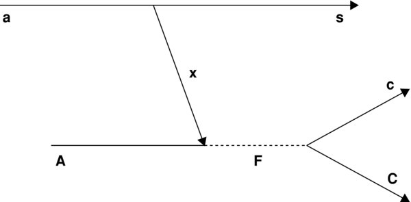
Figure 1. Pole diagram of the a + A → s + c + C resonant QF process. Nucleus a breaks up into fragments x and s. The former is captured by A, leading to the formation of the compound system F, while s flies away without influencing either the A + x → F fusion or the F → c + C decay.
Download figure:
Standard image High-resolution imageThe triple differential cross section of the TH reaction in the c.m. system is given by Dolinsky et al. (1973)
where  . Inserting Equations (3) and (4), integrating Equation (5) over
  , and using the orthogonality properties of the spherical functions and the Clebsch–Gordan coefficients, we obtain the TH double differential cross section:
where  is the differential cross section for the stripping A(a, s)F to the resonant state F
Equation (6) is basic and all the other equations can be obtained from it. This equation explains the advantage of the THM for resonant reactions. To understand it, we compare the TH double differential cross section with the free resonant reaction cross section (all the particles in the initial and exit channels are on-the-energy shell, OES):
It is the expression for the total cross section of the reaction proceeding through an isolated resonance in the R matrix approach, the 18O(p, α)15N reaction in the case under consideration.
We note that in the R matrix approach all the widths depend on the energy, while in the Breit–Wigner expression they are constants taken at the resonance energy. The resonant cross section depends on the entry resonance width, which in the R matrix method can be written as  , where
  is the Coulomb-centrifugal barrier penetrability factor in the channel x + A with relative orbital angular li, depending on ExA and channel radius r0, and γxA is the observable partial reduced width in the channel x + A.
Due to the presence of the penetration factor, the measurement of the resonant cross section at ExA → 0 becomes very difficult or often impossible. The TH double differential cross section  has a structure similar to the R matrix resonant cross section (Equation (8)). The only difference is that the former contains the transfer reaction cross section
  rather than the entry width ΓxA(ExA). The transfer cross section does not go to zero when ExA → 0. Moreover, because in the THM the EaA energy in the entry channel of the TH reaction is chosen to be above the Coulomb barrier,
  is not small making it possible to measure the TH reaction cross section at any small ExA, including ExA = 0 and even ExA < 0. In the THM, absolute cross sections are not measured, nevertheless the free resonant cross section can be obtained by normalization of the TH cross section to the available direct measurements at higher energies assuming that
  is known. Such normalization, given by
provides the resonant cross section (or astrophysical factor) down to energies relevant to astrophysics where direct data are not available or, if available, may be distorted by the electron screening, low-lying unknown resonances or even subthreshold resonances. When two isolated resonances are present, only one of which is known from direct measurements, one can deduce the strength and the astrophysical factor of the unknown resonance by comparing the cross sections of the two resonances observed via the TH reaction.
The two crucial achievements of the resonant THM theory are the possibility of including the effect of distortion due to, for instance, the Coulomb interaction and of calculating the normalization constant needed to compare the direct with the THM data. In turn, these have important consequences as the deduced cross sections or resonance strengths can be calculated with unprecedented accuracy and a further cross check of the method is at hand. In fact, the trend of direct and indirect data can be compared to assess not only the method but also the absolute values of the cross sections.
Here, we use the TH reaction 2H(18O, α15N)n to determine the reaction rates for the 18O(p, α)15N resonant astrophysical process. The deuteron is used as a TH particle to bring the proton inside the nuclear field of 18O. With reference to Figure 1, a ≡ 2H, A ≡ 18O, c ≡ 4He, C ≡ 15N, and x ≡ p, s ≡ n are the participant and the spectator particles, respectively. Therefore, the 2H(18O, α15N)n 2 → 3 reaction can be regarded as the stripping to a resonant state in 19F, later decaying into α + 15N. To measure the energy dependence of  enforcing the QF kinematics (knp = 0) requires a continuous change of beam energy. In the practical realization of the THM, the beam energy is fixed but knp is allowed to vary in the interval of a few tens of MeV/c to span the energy interval relevant for astrophysics (La Cognata et al. 2007b). The chosen 18O beam energy of 54 MeV (La Cognata et al. 2008c) is above the Coulomb barrier allowing for the deuteron to penetrate into the close proximity of 18O. Besides, at this energy the 18O-d relative wavelength
  fm, which is about three times smaller than the deuteron radius. This means that the incident 18O nucleus interacts only with the proton, leaving the second fragment (neutron) as a spectator to the 18O(p, α)15N binary sub-process (the one of astrophysical relevance).
3. THE EXPERIMENT
3.1. Experimental Setup
The experiment was performed at Laboratori Nazionali del Sud, Catania (Italy), and represents the continuation of the one carried out at the Cyclotron Institute, Texas A&M University, Texas (USA) (La Cognata et al. 2008b). The SMP Tandem Van de Graaf accelerator provided a 54 MeV 18O beam, which was accurately collimated in order to achieve a beam spot on the target of about 1 mm diameter, while the maximum beam divergence was 0 08. The intensity was 5 enA on the average and the relative beam energy spread was about 10−4. Thin self-supported deuterated polyethylene (CD2) targets, ≲100
  thick, were adopted in order to minimize energy and angular straggling (about 006) and were placed at 90° with respect to the beam direction. The detection setup, sketched in Figure 2, consisted of a telescope (A), devoted to 15N detection, made up of an ionization chamber (IC) and a silicon position sensitive detector (PSD A) on one side with respect to the beam direction. The telescope was placed at a distance of about 47 cm from the target (upper part of Figure 2). The ionization chamber was used to discriminate nitrogen nuclei by means of the standard ΔE − E technique. In order to minimize the angular straggling in PSD A, a 0.9 μm thick Mylar foil was used as the entrance window; the opposite side was closed by a 1.5 μm thick Mylar foil. The IC was filled with 50 mbar butane gas that provided an energy resolution of about 10%, which was enough to discriminate the impinging particles according to their nuclear charge but not their mass. No threshold was introduced in the 15N detection by the ionization chamber. Three additional silicon PSDs (B, C, and D) were placed on the opposite side with respect to the beam direction, at a distance of about 37 cm from the target (lower part of Figure 2). The distances were chosen to keep the intrinsic angular resolution better than 008, allowing at the same time to cover the relevant angular regions for the subsequent analysis. Angular conditions were selected in order to maximize the expected QF contribution. Indeed, they were chosen to cover momentum values of the undetected neutron ranging from 0 to 150 MeV/c. Thus, the bulk of the QF contribution for deuteron breakup fell inside the investigated region because the momentum distribution for the n − p system has a maximum at ps = 0 MeV/c. The angles corresponding to this condition are known as QF angles. The wide explored momentum range allows for a cross check of the method inside and outside the phase-space regions where the QF contribution is expected. To decrease detection thresholds, no ΔE detectors were put in front of PSDs B, C, and D. Therefore α-particle identification was done from the kinematics of the events. A similar procedure was employed to single out the different nitrogen isotopes detected in telescope A. Energy and emission angle of the detected α's and the emission angle of 15N nuclei were used in the subsequent analysis to enhance energy resolution. Three kinds of events were triggered by using a time-to-amplitude converter (TAC): A–B, A–C and A–D coincidences. Energy and position signals of the PSDs were processed by standard electronics together with the TAC signal for each coincidence event and sent to the acquisition system for on-line monitoring and data storage for off-line processing.
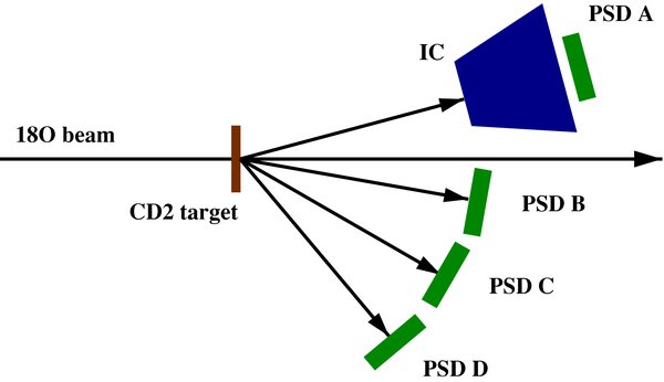
Figure 2. Sketch of the experimental setup. A 54 MeV 18O beam impinges onto a ∼100 μg cm−2 CD2 target and the reaction products are detected in coincidence by means of a ΔE − E telescope (made up of an ionization chamber IC and a silicon position sensitive detector PSDA) and three additional silicon position sensitive detectors PSDB-D.
Download figure:
Standard image High-resolution imageAt the initial stage of the measurement, masks with a number of equally spaced slits were placed in front of each PSD to perform position calibration. The angle of each slit with respect to the beam direction was measured by means of an optical system, making it possible to establish a correspondence between position signal from the PSDs and detection angle of the impinging particles. Energy calibration was performed by means of a standard three-peak α-source (239Pu, 241Am, and 244Cm) and by using the α particles from the 2H(18O,α)16N reaction at 54 MeV, feeding a large number of 16N excited states. Additional runs were performed using a 14N beam at energies ranging between 20 and 50 MeV to measure the elastic and inelastic scattering on gold and carbon targets. This allowed an accurate calibration of PSD A, optimized for nitrogen nuclei detection, and of the IC, by difference in the residual energy measured by PSD A when the IC is empty and filled with butane at the working pressure. The total kinetic energy of the detected particles was reconstructed off-line, taking into account the energy loss in the target and in the entrance and exit windows of the ionization chamber and in the other dead layers.
3.2. Reaction Channel Selection
Since different reactions can be induced by the 18O beam on the measurement target, the reaction channel selection is mandatory. This is accomplished by gating on the coincidence peak in the TAC spectrum for each coincidence couple and by carrying out a careful investigation of the reaction kinematics. This is required to disentangle the events corresponding to the 2H(18O, α15N)n reaction since only a partial particle identification was permitted by the experimental setup, as pointed out in the previous section. Figure 3 displays the particle-identification two-dimensional spectrum provided by telescope A, where the different reaction products are well distinguished in Z but not in A. In detail, the channel selection procedure begins with the separation of the nitrogen locus in the ΔE − E two-dimensional plot by means of a graphical cut. It is well known that particles from a reactions with three nuclei in the exit channel have kinetic energies that are correlated (bound by energy and momentum conservation equations). Therefore, EA versus EB, EA versus EC and EA versus ED (EI, I = A, B, C, D, being the energy measured in the Ith detector) correlation plots were drawn for those events belonging to the nitrogen locus in Figure 3. As an example, the EA versus EC energy correlation plot is given in Figure 4. Three different kinematic loci show up in the picture. The events corresponding to the 2H(18O, α15N)n TH reaction were singled out by comparison with a Monte Carlo simulation of that process, taking into account detection thresholds, energy losses and the kinematics of the TH reaction. The two additional spots located in the upper part of Figure 4 (marked with A and B) correspond to binary reactions that constitute an easily removable background to the TH reaction. Indeed, to rule out these additional channels contributing to the experimental kinematical loci, a graphical cut is introduced in Figure 4 leaving outside of the kinematical regions of interest the contaminant events. A similar approach is pursued for the two A–B and A–D coincidences. In the present experiment, only two of the three emitted particles were detected. This leaves the system underdetermined due to the overlapping of different kinematic loci in the same phase-space region, corresponding to reactions having different undetected particles. To identify the mass of the undetected particle s, the procedure discussed by Costanzo et al. (1990) was applied on the events extracted with the procedure followed until now. Since its momentum is deduced from the energies and emission angles of particles c and C by applying the momentum conservation equation, the variable X = p2s/2u is independent of the mass of the undetected fragment s (u being the unit mass in a.m.u.). If we define Y = Ebeam − Ec − EC, the energy conservation equation can be cast in the form:
thus the mass of particle s can be inferred by fitting the line that best reproduces the experimental data. Therefore, this test allows for a comparison of the expected locus (a straight line) with the experimental one, and it establishes the mass of s with no need of a measurement. Indeed, events from reactions where a bad identification of the detected ejectiles is carried out do not gather along a straight line as Equation (10) does not apply. Its application is demonstrated in Figure 5 for the actual 2H(18O, α15N)n reaction and the A–C coincidence detectors. Clearly, events gather along a straight line whose slope is 1, allowing us to assert that no contaminating kinematics overlap, namely no additional channels contribute to the experimental kinematic locus. This result was supported by the experimental Q-value spectrum where a single peak is apparent, centered at an energy of about 1.75 MeV. The Q-value spectrum for these events is given in Figure 6. The good agreement between the experimental and the theoretical Q-values (indicated by an arrow in Figure 6) confirms not only the identification of the reaction channel but also the accuracy of the performed calibration. Similar results are deduced from the A–B and A–D pairs. In the following, data analysis is restricted to such events.

Figure 3. ΔE − E two-dimensional spectrum from telescope A for particle charge identification. ΔEA and EA are the IC and PSDA signals, respectively.
Download figure:
Standard image High-resolution image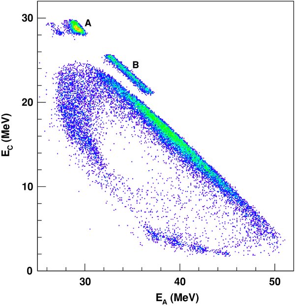
Figure 4. EA − EC two-dimensional spectrum with selection of nitrogen nuclei (Z= 7) on the ΔE − E two-dimensional spectrum in Figure 3. A and B mark two loci corresponding to two-body background reactions.
Download figure:
Standard image High-resolution image
Figure 5. Identification of particle s according to the procedure of Costanzo et al. (1990), applied to the PSDA–PSDC coincidences. In the axes, Y = Ebeam − Ec − EC and X = p2s/2u, where Ec and EC are the energies of α and 15N nuclei, while ps is the momentum of the undetected particle s from momentum conservation. Energy conservation implies  ; thus, the mass of s can be determined.
Download figure:
Standard image High-resolution image
Figure 6. Reconstructed Q-value spectrum. The Q-value for the 2H(18O, α15N)n is marked by an arrow. No additional process takes place as a single peak shows up in the spectrum.
Download figure:
Standard image High-resolution image3.3. Selection of the QF Reaction Mechanism
A further study on reaction dynamics was necessary to select those kinematical regions where QF is dominant and can be separated from possible direct breakup (DBU) or sequential decay (SD) reaction mechanisms. This is an essential step because the equations we have derived are valid only under the assumption that particle s, namely the neutron, acts as a spectator to the A–x interaction. This is accomplished by a thorough study of the reaction dynamics to disentangle the different processes feeding the exit channel, in the same way a study of the reactions kinematics was demanded to figure out the contribution from contaminant reaction channels.
To carry out this study, relative energies for the α − n, 15N − n, and 15N − α systems were deduced from the measured energies and emission angles. In the case of the neutron, these quantities were deduced from the reaction kinematics. Of course, the relative energy spectra represent the excitation energy spectra for 5He, 16N, and 19F nuclei, respectively, above the threshold for neutron or α decay. It means that if any state in such compound systems has been fed in the investigated phase-space region, a bump in the reaction yield should show up at the energy corresponding to the populated excited level. To point out the occurrence of different levels in the same phase-space interval, two-dimensional plots for any two of the three final particles were reconstructed. Relative energies E and E
and E are given in Figure 7 as a function of Eα−n relative energy for the A–C coincidence (upper and lower panels, respectively). No vertical loci show up, corresponding to resonances in the 5He compound nucleus, making us confident that the 2H(18O, α15N)n reaction does not proceed through the 2H + 18O → 5He + 15N → 4He + 15N + n two-step (5He-SD) process. Similarly, the 2H + 18O → 4He + 16N → 4He + 15N + n two-step reaction would lead to the formation of an intermediate 16N excited system (SD mechanism). Since no horizontal loci are apparent in the upper panel of Figure 7, we can conclude that in the examined phase-space region the 16N sequential decay is a less favored process. We can state that such sequential processes (through 5He and 16N) give a negligible contribution to the coincidence yield at α − 15N relative energies corresponding to the region of interest for astrophysics, i.e. around E
 MeV. Similar results are obtained from A–B and A–D coincidences. On the other hand, a large number of 19F excited states are fed in the experiment. This is demonstrated by the lower panel of Figure 7, where several horizontal loci are apparent. These levels can be formed either through the QF reaction mechanism, sketched in Figure 1, following deuteron direct breakup, or via a two-step SD process. Thus, the occurrence of sequential mechanisms in the α − 15N channel cannot be ruled out by studying the relative energy correlation plots only, because the same excited states of the α − 15N system can be formed through a QF or SD process.
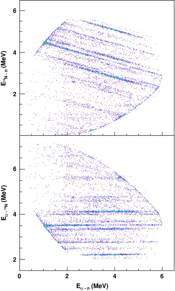
Figure 7. Energy correlation two-dimensional spectra. E , E
, E , and Eα−n are the 15N − n, 15N − α, and α − n relative energies, respectively. Horizontal loci in the lower panel correspond to 19F excited states. No additional loci are apparent, i.e., no sequential decay process is contributing.
Download figure:
Standard image High-resolution imageA way to discriminate between SD and QF events is through the study of the reaction yield as a function of the neutron momentum ps. Indeed, an enhancement of the cross section close to zero neutron momentum is a necessary condition for the occurrence of the QF mechanism, marking the presence of a modulation of the TH cross section by the neutron momentum distribution inside the deuteron. This feature is expected for a QF reaction because the momentum distribution of the n − p system inside the deuteron has a maximum for ps = 0 MeV/c. Since the experimental range of the spectator particle momentum extends well beyond the interval where the QF contribution is supposed to be dominant, namely outside the full width at half maximum of the Hulthén momentum distribution (FWHM = 72 MeV/c), a comparison of the coincidence yield for small ps (say, ≲FWHM/2 = 36 MeV/c) and larger ps can be performed. For this purpose, the behavior of the coincidence yield spectra as a function of Ec.m. was reconstructed for all coincidence events, for different neutron momentum ranges. Ec.m. is the 18O − p relative kinetic energy related to  relative energy by the energy conservation law:

where Q2 = 3.981 MeV is the Q-value of the 18O(p, α)15N reaction (see, e.g., Spitaleri et al. 2004 and references therein). In detail, these spectra, given in Figure 8, were obtained by selecting the |ps| < 20 MeV/c (upper panel), 20 < |ps| < 40 MeV/c (middle panel), and 40 < |ps| < 60 MeV/c (lower panel) intervals of the neutron momentum ps. Furthermore, such spectra were divided by the phase-space contribution to remove the pure kinematical effects due to the phase-space selection. In the picture, only the Ec.m. range of interest for astrophysics is displayed, namely Ec.m. < 250 keV; in this range, the resonances corresponding to the 8.014, 8.084, and 8.138 MeV states in the 19F compound nucleus (Tilley et al. 1995) show up. It is important to stress that the Ec.m. spectra given in Figure 8 are not corrected for the modulation given by the angular dependence in Equation (5). Therefore, the distinguishing pattern due to the ps dependence can be unveiled only in the case of isotropic resonances. Since this condition is satisfied only for the 8.138 MeV state in 19F (Tilley et al. 1995; Lorentz-Wirzba et al. 1979), we will focus on this level, corresponding to a resonance at Ec.m. = 144 keV that is clearly visible in Figure 8. Such a picture clearly demonstrates that in the energy region around 144 keV, the coincidence yield is much higher for |ps| < 20 MeV/c than what is obtained at larger ps momenta. Indeed, at higher momenta (20 < |ps| < 40 MeV/c and 40 < |ps| < 60 MeV/c) it drastically decreases and the resonance becomes barely visible compared to the background. These data provide strong evidence of a clear correlation between coincidence yield and spectator momentum ps, which is a necessary condition for the occurrence of the QF reaction mechanism.
Figure 8. Normalized reaction yield for different ps ranges. The reaction yield monotonically decreases moving to high ps values, as expected for a QF reaction using deuteron as TH nucleus. This represent a first test of the occurrence of the QF mechanism in the 2H(18O, α15N)n reaction.
Download figure:
Standard image High-resolution imageThe previous discussion can be made more quantitative as the neutron momentum distribution inside the deuteron can be measured by means of the 2H(18O, α15N)n QF reaction. Indeed, only if the deuteron breakup process is direct, the neutron momentum distribution keeps the same shape as inside d. Thus, the agreement between the shape of the deuteron momentum distribution and the experimental one is a compelling evidence of the occurrence of the QF mechanism (Spitaleri et al. 1999, 2004; La Cognata et al. 2007b). To establish the momentum dependence of the coincidence yield, the modulation due to the feeding of states in 19F (compare Figure 8) has to be removed, which otherwise would conceal the trend that is much weaker than the resonant structure. This is accomplished by fixing the E relative energy at the top of the resonant peak at Ec.m. = 144 keV, corresponding to the 8.138 MeV state in 19F, which is clearly visible in Figure 8. Phase-space effects were divided out as in the previous case, by performing a Monte Carlo simulation of the experimental setup, accounting for the covered angular ranges in the experiment and for the detection thresholds. Furthermore, no angular distribution modulation is expected as the 19F decay from such a state is isotropic, as observed before. Thus, the experimental ps momentum distribution is obtained in arbitrary units and displayed in Figure 9 by solid dots. This result is compared with the square of a Hulthèn wave function in momentum space (Zadro et al. 1989; Spitaleri et al. 2004; La Cognata et al. 2007b), representing the shape of the n − p momentum distribution in the plane-wave impulse approximation (PWIA):
with parameters a = 0.2317 fm−1 and b = 1.202 fm−1 (Spitaleri et al. 2004; La Cognata et al. 2007b) for the deuteron. Since the experimental momentum distribution is known in arbitrary units only, the theoretical one has been scaled to the experimental maximum (Figure 9), for comparison ( ). This is given in Figure 9 as a black solid line. As regards the width, the experimental FWHM should coincide with the predicted one, about 72 MeV/c (Zadro et al. 1989) because of the large transferred momentum. Distortions, if any, should influence only the tails of the distribution (Spitaleri et al. 2004), beyond the range of interest, corresponding to short n − p relative distances, as only the nuclear interaction can influence the p–18O interaction. To check whether the simple PWIA approach gives an accurate description of the n − p momentum distribution, in Figure 9 the DWBA distribution, evaluated by means of the FRESCO computer code (Thompson 1987), is also given by a red dotted line. Again, the theoretical DWBA momentum distribution has been scaled to the experimental maximum for easier comparison (
 ). In the calculation, optical potential parameters extrapolated from the Perey & Perey (1976) compilation have been adopted. From the comparison we can state that a good agreement between the two is present for a neutron momentum ps < 50 MeV/c, which is within the experimental uncertainties (including only the statistical error, in the case of Figure 9). This demonstrates that the PWIA approach constitutes a viable approach to extract the resonance parameters for the 18O(p, α)15N reaction. In fact, according to the resonant THM outlined in the beginning, the 2 → 3 cross section used to extract the resonance strengths is integrated over ps; thus, distortions would provide a contribution as small as 4% to the overall error budget. The DWBA momentum distribution accounts for the shape of the experimental distribution, which is slightly narrower than expected from the PWIA prediction. This effect has been systematically observed in several works (Pizzone et al. 2009) and finds a natural and simple explanation in the present approach. Moreover, such an agreement means that the QF mechanism is present and dominant in the ps < 50 MeV/c neutron momentum range. For these reasons, in the following analysis, only the phase-space region where ps < 50 MeV/c is taken into account, allowing us to apply the PWIA in the following calculations without introducing significant systematic uncertainties. Together with the previous tests, the good agreement between the theoretical and experimental distributions makes us confident that the QF mechanism gives the main contribution to the 18O+d reaction at an energy of 54 MeV in the experimental kinematical regions. Moreover, it proves that the QF mechanism can be selected without significant contribution from contaminant SD processes and the analysis in PWIA is sufficient to describe the process.
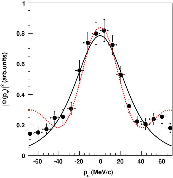
Figure 9. Experimental momentum distribution (full dots) compared with theoretical ones, given by the square of the Hulthén wave function in momentum space (black solid line) and by the DWBA momentum distribution evaluated by means of the FRESCO code (red dotter lines). Normalization was left as a fitting parameter.
Download figure:
Standard image High-resolution image4. RESULTS
4.1. Angular Distributions and Spin-parity Assignment
According to La Cognata et al. (2007b), Spitaleri et al. (2004), and La Cognata et al. (2008c), the comparison between the angular distribution of the fragments α and 15N, measured from the 2H(18O, α15N)n TH reaction, and those expected from the OES resonant 18O(p, α)15N reaction, provides another validity test for the THM because it would mean that no distortions are induced by the emitted neutron. In this work, the angular distributions of the final fragments coming from the 18O(p, α)15N subreaction are extracted not only to validate the THM approach but also to evaluate spin and parity of the low-laying resonances. Note that in the case of the 144 keV resonance corresponding to the 8.138 MeV state in 19F, the angular distribution was directly measured by Lorentz-Wirzba et al. (1979). Conversely, since the spin–parity of the 90 keV resonance (namely the 8.084 MeV excited state of 19F) is not well established (Tilley et al. 1995), a close examination of the angular distribution should allow to pin down the correct values. The invariant scattering angle in direct measurements is determined as the angle between the relative momenta of the final and initial particles. In the c.m. system of the subreaction, such an angle is the one between the momentum of any of the two fragments (α or 15N) and the beam direction. The emission angle for the 15N nucleus is given by

where the relative momenta  are invariant under Galilean transformations, i.e., they remain the same in any coordinate system. Hence, they can be calculated using the momenta in the laboratory system, where the momentum of the transferred proton is equal and opposite to that of neutron in the QF kinematics (Jain et al. 1970; La Cognata et al. 2007b; Spitaleri et al. 2004).
The general expression for the angular distribution of the fragments for the resonance reaction has been obtained by Blatt & Biedenharn (1952). In the case of an isolated resonance with only one value of li, lf, Si, and Sf, it takes the form
In this equation,  and
and  are Wigner 6j-symbols (Messiah 1962a),
  and
and  Clebsch–Gordan coefficients (Messiah 1962b). K is a normalization constant, which in general is a function of the c.m. energy Ec.m..
Because of the different phase-space regions explored in the present experiment, the θc.m. ranges for the A–B, A–C, and A–D detector coincidences were about θc.m. = 0°–60°, θc.m. = 40°–110°, and θc.m. = 90°–150°, respectively. The presence of the overlap regions allowed to normalize the cross sections deduced from each couple to one another. Angular distributions were extracted for several energies, focusing in particular on the 0–250 keV energy region, where the 20 keV, 90 keV, and 144 keV resonances occur. As discussed below, the experimental energy resolution was about 17 keV. Therefore, the extraction of the angular distributions for each resonance cannot be accomplished at fixed energy. Moreover, the 90 keV and the 144 keV resonances partially overlap; thus, care has to be taken to disentangle contributions from different peaks. Consequently, the excitation functions were deduced in 10 degree bins for the whole explored angular range, following the technique extensively discussed by Spitaleri et al. (2004) and La Cognata et al. (2007b). The half-off-energy-shell (HOES) cross section (dσ/dΩc.m.)HOES for the 18O(p, α)15N reaction, as a function of energy and for a fixed θc.m. angle, was derived by dividing the selected coincidence yield by the result of a Monte Carlo calculation, which was carried out to evaluate the KF |Φ(ps)|2 product. The momentum distribution in the calculation is shown in Figure 9 and a cutoff ps < 50 MeV/c neutron momentum range was introduced to single out the QF kinematic region. The HOES label is used as the transferred proton is off-the-energy-shell while the other particles are real. As reported by Spitaleri et al. (2004) and La Cognata et al. (2007b), the HOES nature of the measured cross section has no influence on the angular distributions since they are extracted for fixed energies and in arbitrary units. The K factor in Equation (14), which reflects the HOES nature of the differential cross section when Equation (14) is used for the HOES angular distributions, is taken as a constant.
The resulting excitation function corresponding to θc.m. = 55° is given in Figure 10 (solid dots) as an example. Clearly, three peaks show up corresponding to the cited resonances; these were fitted simultaneously with three Gaussian curves to separate the contribution to the normalized yield of each resonance. The fitting curves are shown by red solid lines in Figure 10, while the sum of these resonant terms with the nonresonant contribution (which, for the sake of simplicity, is not displayed in Figure 10) is displayed by a black solid line. The same fitting procedure has been repeated for each θc.m. angle to determine the relative population of each resonance depending on the angle. The resulting angular distributions are displayed in Figure 11, where the experimental data are given by filled circles (20 keV), squares (90 keV), and triangles (144 keV). Errors on (dσ/dΩc.m.)HOES account for statistics (∼10%, ∼15%, and ∼5% for the 20, 90, and 144 keV resonances, respectively) and for the deconvolution of the single resonance contributions. This error source is dominant for the 90 keV resonance, as a strong tail from the more intense 144 keV peak makes it more difficult to disentangle the two contributions (see Figure 10). This is especially evident above ∼100°, where the two resonances are less resolved due to the slightly poorer resolution of detector D with respect to the other PSDs. The error on θc.m. represents the width of each bin (chosen in order to have enough statistics per bin, namely 10° in this case). Angular distributions in Figure 11 are given in arbitrary units; in principle, from Equation (6) it would be possible to provide the absolute cross section by simple calculations, but it would require the evaluation of the  differential cross section for the 18O + d → 19F + n stripping process leading to the resonant state of the excited 19F nucleus. This, in turn, requires an estimate of the suited spectroscopic factors, which can introduce large uncertainties in the predicted cross section. For these reasons, a different normalization procedure has been devised, which greatly reduces the uncertainty on the cross section obtained by means of the THM. Accordingly, K is taken as an arbitrary normalization constant in Figure 11.

Figure 10. HOES excitation function (in arbitrary units) for the 18O(p, α)15N reaction obtained for a fixed θc.m. = 55° angle, in the 0–250 keV energy range. A Gaussian fit (red lines) is used to disentangle the contribution of each peak to the overall normalized coincidence yield. The black solid line is the sum of the obtained Gaussian functions and of a straight line (not shown) to provide for the nonresonant contribution (see text for details).
Download figure:
Standard image High-resolution image
Figure 11. Experimental angular distributions for the 18O(p, α)15N reaction for the three resonances in the 0–250 keV energy range. The full lines are the theoretical angular distributions for the free OES 18O(p, α)15N reaction, calculated according to the equations of Blatt & Biedenharn (1952).
Download figure:
Standard image High-resolution imageFrom Figure 11 it turns out that the  assignment for the 144 keV resonance is confirmed, the angular distribution for that level being isotropic (the best fit being given by a straight line, see Figure 11). This result represents a cross check of the method, since we are able to reproduce the angular distribution for a well-known resonance (the differential cross section for it being given by Lorentz-Wirzba et al. 1979). Assuming that the spin–parity assignments of La Cognata et al. (2008c) hold, using Equation (14) we have calculated the angular behavior of the HOES differential cross section for the resonance at 20–90 keV. With respect to the calculation by La Cognata et al. (2008c), the only fitting constant is the K factor, which has been determined by minimizing the χ2. This allows us not only to further check the spin–parity assignment given by La Cognata et al. (2008c) but also to quantitatively determine any deviation from the expected angular distribution for a resonant state, and then to pin down any distortion. This test is feasible since no fitting, except for normalization, is needed (while in the La Cognata et al. 2008c paper the fitting with a simple cosine polynomial was used). The calculated angular distributions are given by solid black lines in Figure 11. Good agreement between the THM data and the theoretical angular distributions makes us confident that
  and
and  spin–parity assignments for the 90 and 20 keV states, respectively, are confirmed. Moreover, the QF conditions are well satisfied since no neutron distortion is apparent. This means that we can proceed to the extraction of the resonance strength for all the requirements of the THM theory are clearly fulfilled.
4.2. Cross Section of the 2H(18O, α15N)n Reaction. Extraction of Resonance Strengths
In order to obtain the cross section for 2H(18O, α15N)n, we use the double differential TH cross section given by Equation (6), which was obtained by integration over the solid angle  . Given the good agreement between the experimental and theoretical angular distributions (Figure 11) throughout the range covered here, the angular integration was performed assuming that the trend of the angular distributions is given by the theoretical one outside the range where our measurements are present. The resulting 2H(18O, α15N)n reaction cross section is shown in Figure 12 (full circles). Here, the error bars arise from statistical uncertainty (about 5%, on the average) and angular distribution integration. This last error accounts for the uncertainties coming from the adopted procedure to disentangle the contribution of each resonance to the reaction yield, as shown in the previous section. From the inspection of Figure 12 (and, clearly, from Figure 10), it turns out that the experimental resolution is much larger than the natural width of 1 keV or less typical of 19F resonances in the 18O(p, α)15N reaction at c.m. energies below 1 MeV (Tilley et al. 1995). Indeed, from the Gaussian fit of the total cross section for the 2H(18O, α15N)n QF process, Figure 12, a resonance FWHM of about 40 keV is obtained for all the resonances (σ ∼ 17 keV). Just for comparison, the well known 144 keV resonance has a natural width Γ ⩽ 0.3 keV; thus, the experimental width coincides with the energy resolution, which can be considered constant in the 0–250 keV energy range as it is the same for all the observed resonances. This experimental value of the energy resolution is corroborated by Monte Carlo simulations, which take into account beam emittance through the collimating system, and energy and angular straggling in the target, ΔE detector and the dead layers along the particle flight path. Such a calculation is of primary importance as the Ec.m. energy is not measured, but rather is indirectly deduced from the kinematics of the 2 → 3 reaction. The main result is that because of the effect of energy resolution, the theoretical 2 → 3 QF cross section as deduced in the THM approach (see Equation (6), assuming that nonresonant contributions are negligible), namely
is not directly observable. More precisely, even though the ideal resolution resonance shape cannot be observed, the effect of energy resolution will enable us to directly extract the strengths of the low-energy resonances. In Equation (15), ![$\frac{{\rm d}\sigma _{[d({}^{18}{\rm O}, {}^{19}{\rm F}_{i})n]}}{{\rm d}\Omega _{n}}$](https://content.cld.iop.org/journals/0004-637X/708/1/796/revision1/apj328571ieqn47.gif) is the differential cross section for the transfer reaction 18O + d → 19Fi + n populating the ith resonant state in 19F with the resonance energy
is the differential cross section for the transfer reaction 18O + d → 19Fi + n populating the ith resonant state in 19F with the resonance energy  ,
,  is the partial resonance width for the decay 19Fi → α + 15N and Γi is the total resonance width of the ith resonance in the 19F compound nucleus (La Cognata et al. 2007b; Mukhamedzhanov et al. 2008). It is worth stressing that
  does not appear in Equation (15), where the transfer reaction cross section
 ![$\frac{{\rm d}\sigma _{[d({}^{18}{\rm O}, {}^{19}{\rm F}_{i})n]}}{{\rm d}\Omega _{n}}$](https://content.cld.iop.org/journals/0004-637X/708/1/796/revision1/apj328571ieqn51.gif) shows up instead. The great advantage is that Coulomb barrier penetrability factor is missing; thus, it is possible to extend the measurement down to zero Ec.m. energy. This is the reason why the THM has been developed. However, this is also a drawback of the method, as there is no sensitivity on the entrance channel partial width, which has to be calculated, for instance, by means of the usual formula (Champagne & M. Pitt 1986) (for the 18O + p channel):
shows up instead. The great advantage is that Coulomb barrier penetrability factor is missing; thus, it is possible to extend the measurement down to zero Ec.m. energy. This is the reason why the THM has been developed. However, this is also a drawback of the method, as there is no sensitivity on the entrance channel partial width, which has to be calculated, for instance, by means of the usual formula (Champagne & M. Pitt 1986) (for the 18O + p channel):
as described in the introduction. The total cross section, as given in Figure 12, clearly represents the convolution of the TH cross section given by Equation (15) with the finite resolution. As it is demonstrated in the Appendix, the experimental THM cross section for the 2H(18O, α15N)n QF process is given by Equation (A5), which we report here:
According to Equation (A4), the Ni parameters represent the TH resonance strengths. In what follows, the sum is extended to the three non-interfering resonances in the 0–250 keV Ec.m. range, corresponding to the 8.014, 8.084, and 8.138 MeV states in the 19F compound nucleus (Tilley et al. 1995). These levels are marked in Figure 12 by arrows. A first-order polynomial has been added to account for nonresonant contributions. Equation (A5) has been adopted to fit the experimental data, with the aim of extracting the Ni parameters that bear a fundamental physical meaning. In fact, they are easily connected to the resonance strengths (ωγ)i for the ith 19F level (Rolfs & Rodney 1988), which are the key parameters to evaluate the reaction rate for the astrophysical application in the case of narrow resonances. Since the TH cross section is given in arbitrary units in Figure 12, the Ni parameters need to be normalized to get the resonance strengths, as we will discuss later. Following (Rolfs & Rodney 1988), we define the resonance strength for the ith state as follows:
where the first fraction on the right-hand side is the statistical factor ωi,  ,
,  , Jp, and Ji being the spin of the 18O nucleus, of the proton and of the intermediate 19F resonance through which the reaction proceeds. In the second fraction on the right-hand side of Equation (17),
  and
and  are the partial widths for the p + 18O → 19Fi and 19Fi → α + 15N channel, leading to the population of the ith excited state in 19F or following its decay, respectively. Finally,
  is the total width of the ith resonance in the 19F compound nucleus. The latter ratio represents the so-called γi of the resonance. From Equations (A4) and (17), a simple connection between the Ni terms, experimentally determined by means of the THM, and the resonance strength (ωγ)i of the ith resonance, can be established:
taking  for short. This result represents the main achievement of the present work; the resonance strengths can be deduced with no need of introducing spectroscopic factors, thus greatly reducing the uncertainties affecting resonance strengths when indirectly established. As we have described in the introduction, this is the sole possibility whenever the resonance under study occurs well below the Coulomb barrier, where barrier penetration strongly suppresses the reaction cross section (compare, for instance, Champagne & M. Pitt 1986; Wiescher & Kettner 1982). In Equation (18), the spectroscopic factor for the ith resonance does not appear because it cancels out in the
 ![$\Gamma _{(p{}^{18}{\rm O})_{i}}/({\rm d}\sigma _{[d({}^{18}{\rm O},{}^{19}{\rm F}_{i})n]}/{\rm d} \Omega _{n})$](https://content.cld.iop.org/journals/0004-637X/708/1/796/revision1/apj328571ieqn58.gif) ratio. In fact, from Champagne & M. Pitt (1986), for instance, it turns out that
ratio. In fact, from Champagne & M. Pitt (1986), for instance, it turns out that  , defined in Equation (16), is proportional to the spectroscopic factor Si of the configuration 18O + p in 19Fi, through the
  factor, which is the dimensionless reduced width that is given by
where r is the nuclear interaction radius and R(r) is the radial form factor. The transfer reaction differential cross section ![${\rm d}\sigma _{[d({}^{18}{\rm O}, {}^{19}{\rm F}_{i})n]}/{\rm d}\Omega _{n}$](https://content.cld.iop.org/journals/0004-637X/708/1/796/revision1/apj328571ieqn61.gif) taken in the DWBA form is also proportional to the spectroscopic factor Si. Here, we use the PWIA to estimate this differential cross section. First of all, the PWIA provides a very reasonable description of the angular distributions of the stripping reactions A(d, p)F populating the resonance states (Dolinsky et al. 1973). It is well known that the PWIA overestimates the absolute value of the differential cross section, but we need to know only the ratio of the differential cross section for the transfer reactions populating two different resonant states rather than the absolute value of the individual transfer cross sections, which makes the PWIA a good approximation. The reaction amplitude in Equation (7) for the population of the ith resonance in 19F in the prior form of the PWIA is given by (for simplicity, we drop the spins of the particles):
taken in the DWBA form is also proportional to the spectroscopic factor Si. Here, we use the PWIA to estimate this differential cross section. First of all, the PWIA provides a very reasonable description of the angular distributions of the stripping reactions A(d, p)F populating the resonance states (Dolinsky et al. 1973). It is well known that the PWIA overestimates the absolute value of the differential cross section, but we need to know only the ratio of the differential cross section for the transfer reactions populating two different resonant states rather than the absolute value of the individual transfer cross sections, which makes the PWIA a good approximation. The reaction amplitude in Equation (7) for the population of the ith resonance in 19F in the prior form of the PWIA is given by (for simplicity, we drop the spins of the particles):
where φd(pnp) is the Fourier transform of the s-wave radial p − n bound-state wave function, ppn is the p − n relative momentum, which is equal to the neutron momentum ps in the system where deuteron is at rest, while
is the form factor for the synthesis 18O + p → 19Fi, leading to the ith excited state in 19F,  is the overlap function of the wave functions of the 18O − p system with the resonance wave function of 19Fi,
  is the 18O + p relative momentum and
  is the 18O − p interaction potential, which depends on the distance between p and c.m. of 18O. In the calculation we approximated
  by
by  , where
  is the single-particle bound-state type wave function describing the 19Fi resonance state. Since we consider the (p, α) resonant reaction, the dominant contribution comes from the nuclear interior where proton and alpha channels are coupled. That is why for the
  wave functions we used an approach similar to the R matrix: these wave functions are taken to be real and calculated as the level wave functions in the nuclear interior. As
  is proportional to the spectroscopic factor Si as well, the
 ![$\Gamma _{(p{}^{18}{\rm O})_{i}}/{\rm d} \sigma _{[d({}^{18}{\rm O},{}^{19}{\rm F}_{i})n]}/{\rm d}\Omega _{n}$](https://content.cld.iop.org/journals/0004-637X/708/1/796/revision1/apj328571ieqn70.gif) ratio is an easily calculable and non-ambiguous quantity.
ratio is an easily calculable and non-ambiguous quantity.
Figure 12. Cross section of the TH reaction (full circles). The full line represents the result of a fit including three Gaussian curves (short-dashed, dotted, and short-dashed dotted lines) and a first-order polynomial (long-dashed dotted line) to take into account the three resonances at 20, 90, and 144 keV and background, respectively.
Download figure:
Standard image High-resolution imageTo determine the Ni parameters, which are needed to evaluate the resonance strengths, the TH cross section (in arbitrary units, see Figure 12) has been fit by means of Equation (A5). The resulting best fit curve is given as a solid black line in Figure 12 while the contribution of the 20 keV, 90 keV, and 144 keV resonances is given by a dashed, dotted, and dot-dashed line, respectively. The nonresonant contribution is also shown by a dot-long-dashed line. This fit yielded the following resonance energies:  keV,
keV,  keV, and
  keV (in fair agreement with the ones reported in the literature; Angulo et al. 1999) and the peak values Ni of each resonance: N1 = 138 ± 8, N2 = 82 ± 9, and N3 = 347 ± 8 (arbitrary units). It is worth stressing that the good quality of the fit with the Gaussian curves proves that our assumption of a Gaussian detector response function is well justified, as clearly demonstrated by Figure 12. The error affecting the Ni parameters accounts for the errors on the measured TH cross section and for the uncertainty on the nonresonant term, which has been determined in a simplified approach. The contribution to the error budget of the nonresonant term is estimated by scaling the fitted polynomial until the resulting curve passes through the top and bottom edges of the error bars given in Figure 12. This provides the maximum and minimum values of the nonresonant contribution allowed by the TH cross section, respectively.
Apart from the ![$\Gamma _{(p{}^{18}{\rm O})_{i}}/{\rm d}\sigma _{[d({}^{18}{\rm O}, {}^{19}{\rm F}_{i})n]}/{\rm d}\Omega _{n}$](https://content.cld.iop.org/journals/0004-637X/708/1/796/revision1/apj328571ieqn74.gif) ratio that is needed to link them to the OES strengths, a normalization constant is required since the TH data are given in arbitrary units. Normalization has been performed by scaling the strengths of the 20 and 90 keV resonances (i = 1 and 2, respectively) to one of the 144 keV (i = 3), which is well known from the literature, as already discussed. Quantitatively, from Equation (18), we obtain
ratio that is needed to link them to the OES strengths, a normalization constant is required since the TH data are given in arbitrary units. Normalization has been performed by scaling the strengths of the 20 and 90 keV resonances (i = 1 and 2, respectively) to one of the 144 keV (i = 3), which is well known from the literature, as already discussed. Quantitatively, from Equation (18), we obtain
By using (ωγ)3 = 0.167 ± 0.012 eV from Becker et al. (1995) in Equation (22), one gets (ωγ)1 = 8.3+3.8−2.6 × 10⁻¹⁹ eV, which is well within the upper and lower limits given by NACRE, 6+17−5 × 10⁻¹⁹ eV (Angulo et al. 1999). The largest contribution to the error is due to the uncertainty of the resonance energy, while statistical, systematic, and normalization errors add up to 9.5%. In detail, systematic errors are related to the model adopted to calculate the single particle partial width and the transfer cross section entering the ![$\Gamma _{(p{}^{18}{\rm O})_{i}}/{\rm d}\sigma _{[d({}^{18}{\rm O},{}^{19}{\rm F}_{i})n]}/{\rm d}\Omega _{n}$](https://content.cld.iop.org/journals/0004-637X/708/1/796/revision1/apj328571ieqn75.gif) ratio, while the normalization error is due to the uncertainty affecting the (ωγ)3 from Becker et al. (1995). With a similar approach, we have obtained (ωγ)2 = (1.76 ± 0.33) × 10−7 eV (statistical and normalization errors ∼13%) for the 90 keV resonance, in good agreement with the strength given by NACRE, (1.6 ± 0.5) × 10−7 eV (Angulo et al. 1999). The adopted normalization procedure has two sizeable advantages. (1) Since the 144 keV resonance is well known, the error on it, which propagates onto the uncertainty affecting the 20 and 90 keV resonances, is smaller than the one coming from the usual normalization procedures, which rely on the measurement of the collected charge, on the thickness of the target, and on solid angles and dead time, for instance, which can be very critical. For this reason, it does not present systematic effects. Indeed, these are difficult to estimate and often constitute the main concern in the determination of cross sections of astrophysical importance. (2) The double ratio compensates for possible systematic errors implied by the experimental procedure, namely those coming from the model assumptions used to calculate the
ratio, while the normalization error is due to the uncertainty affecting the (ωγ)3 from Becker et al. (1995). With a similar approach, we have obtained (ωγ)2 = (1.76 ± 0.33) × 10−7 eV (statistical and normalization errors ∼13%) for the 90 keV resonance, in good agreement with the strength given by NACRE, (1.6 ± 0.5) × 10−7 eV (Angulo et al. 1999). The adopted normalization procedure has two sizeable advantages. (1) Since the 144 keV resonance is well known, the error on it, which propagates onto the uncertainty affecting the 20 and 90 keV resonances, is smaller than the one coming from the usual normalization procedures, which rely on the measurement of the collected charge, on the thickness of the target, and on solid angles and dead time, for instance, which can be very critical. For this reason, it does not present systematic effects. Indeed, these are difficult to estimate and often constitute the main concern in the determination of cross sections of astrophysical importance. (2) The double ratio compensates for possible systematic errors implied by the experimental procedure, namely those coming from the model assumptions used to calculate the ![$\Gamma _{(p{}^{18}{\rm O})_{i}}/{\rm d}\sigma _{[d({}^{18}{\rm O},{}^{19}{\rm F}_{i})n]}/{\rm d}\Omega _{n}$](https://content.cld.iop.org/journals/0004-637X/708/1/796/revision1/apj328571ieqn76.gif) ratio. Thanks to the double ratio in Equation (22), where the
ratio. Thanks to the double ratio in Equation (22), where the ![$\Gamma _{(p{}^{18}{\rm O})_{i}}/{\rm d}\sigma _{[d({}^{18}{\rm O},{}^{19}{\rm F}_{i})n]}/{\rm d}\Omega _{n}$](https://content.cld.iop.org/journals/0004-637X/708/1/796/revision1/apj328571ieqn77.gif) is calculated for two close resonances, the normalized (ωγ)i turns out to depend very weekly on the model and the parameters (single particle wave functions, potential wells, etc.). Usually, to calculate a direct transfer reaction amplitude, the DWBA is used, but to estimate the ratio of two direct reaction amplitudes, it is sufficient to use the plane-wave approximation. In fact, the plane-wave approximation has a similar angular and energy dependence as the DWBA but it significantly overestimates the absolute value of the cross section, so this issue is definitely by-passed if normalization is achieved by scaling to the known 144 keV resonance strength. Therefore, the plane-wave assumption turns out to be fully justified as no absolute values are required.
is calculated for two close resonances, the normalized (ωγ)i turns out to depend very weekly on the model and the parameters (single particle wave functions, potential wells, etc.). Usually, to calculate a direct transfer reaction amplitude, the DWBA is used, but to estimate the ratio of two direct reaction amplitudes, it is sufficient to use the plane-wave approximation. In fact, the plane-wave approximation has a similar angular and energy dependence as the DWBA but it significantly overestimates the absolute value of the cross section, so this issue is definitely by-passed if normalization is achieved by scaling to the known 144 keV resonance strength. Therefore, the plane-wave assumption turns out to be fully justified as no absolute values are required.
For the first time, thanks to the novel approach developed here, which allows one to fully account for distortions in the entrance and exit channel, the uncertainty due to the theoretical calculation has been evaluated. In the DWBA framework, it has been found that it contributes to the overall error budget with a ∼10% additional error, which contains a 4% contribution from the chosen wave functions and a 5% due to the possible choice of the interaction radius. This figure represents an upper limit since the errors partially compensate as they appear in a ratio. This is a key result both for astrophysics and for THM application, as it shows the accuracy of the extracted ωγ and the robustness of the method.
Finally, we underscore that the electron screening effect gives a negligible contribution around 144 keV (4% maximum; Assenbaum et al. 1987); thus, no systematic uncertainty is introduced by normalizing to the third resonance due to the shielding of atomic nuclei. This is to confirm what we stated in the initial sections, namely the THM provides an electron-screening-free astrophysical S(E) factor.
4.3. Evaluation of the Reaction Rate
To calculate the reaction rate for the 18O(p, α)15N reaction, we have applied the narrow resonance approximation (see, e.g., Angulo et al. 1999; Rolfs & Rodney 1988), which is fulfilled for the resonances under investigation, the width of the studied resonances being typically about 1 keV or less. According to this approximation, the contribution to the rate of the ith resonance is determined as follows:
where μ is the reduced mass for the projectile-target system, T is the temperature of the astrophysical site, and  is measured in cm3 mol−1 sec−1. The contributions to the overall 18O(p, α)15N reaction rate of the 20 keV and 90 keV resonances are given by dashed and dot-dashed lines, respectively, in Figure 13, as a function of T9 = T/109 K. In the same figure, the total reaction rate is displayed by a solid line for comparison. The contribution to the total rate of higher energy resonances in the 18O(p, α)15N spectrum, as well as the nonresonant component of the cross section, is taken the same as in the NACRE compilation (Angulo et al. 1999). Figure 13 clearly shows that the 20 keV resonance provides a critical contribution at the lowest temperatures, where it dominates the reaction rate. On the other hand, the role of the 90 keV resonance turns out to be negligible over the whole temperature range. Because of the steep descent of
  with decreasing temperature (for a factor 10 change in the temperature, the reaction rate drops by about 30 orders of magnitude), the modification in the reaction rate due to the resonance strengths determined here cannot be appreciated. To compare the present results with the one reported in the NACRE compilation (Angulo et al. 1999), the ratio of the TH reaction rate to the NACRE one for the 18O(p, α)15N reaction has been evaluated. The result is shown in Figure 14 by a full black line. The dot-dashed and dotted black lines represent the upper and lower limits, respectively, allowed by the experimental uncertainties for the TH reaction rate. In this representation, the NACRE rate is given by a full red line, equal to 1 in the plotted temperature range. As before, the dot-dashed and dotted red lines represent the range allowed by the uncertainties affecting the NACRE rate. In particular, to make the comparison consistent, only the uncertainty due to the 20 keV and 90 keV resonance contributions to the reaction rate is taken into account. In the lower temperature region (below T9 = 0.03, Figure 14(a)), the reaction rate can be up to ∼35% larger than the one given by NACRE, while the uncertainty is greatly reduced with respect to the NACRE one. Indeed, the present approach has reduced the error due to the poor knowledge of the parameters of the 20 keV resonance in the 18O(p, α)15N reaction by a factor ∼8.5. These temperatures are typical of the bottom of the convective envelope. Thus, an increase of this reaction rate might have important consequences on extra mixing mechanisms (Nollett et al. 2003) and, in turn, on the surface abundances and isotopic ratios in AGB stars. In the higher temperature region (above T9 = 0.03, Figure 14(b)), an increase of less than 1% is obtained due to the TH measurement of the low-laying-level resonance strengths. This is because the 8.084 MeV excited state of 19F (corresponding to the 90 keV resonance) provides a negligible contribution to the reaction rate, in agreement with the previous estimate by Champagne & M. Pitt (1986).
Figure 13. Decimal logarithm of total reaction rate of the 18O(p, α)15N reaction (solid line), together with the contributions of the 20 keV and 90 keV resonances (dashed and dot-dashed lines, respectively).
Download figure:
Standard image High-resolution image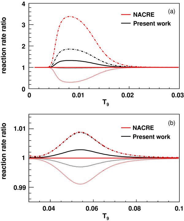
Figure 14. Comparison of the THM reaction rate of the 18O(p, α)15N reaction with the NACRE one (Angulo et al. 1999). The full red line is the reference NACRE rate, while the full black line is the THM rate. The dot-dashed and dotted lines give the upper and lower limits allowed by uncertainties, respectively. Again, red and black lines denote the NACRE and THM results, respectively.
Download figure:
Standard image High-resolution image
5. CONCLUDING REMARKS
In this work, a reanalysis of the 18O(p, α)15N reaction, investigated by means of the THM applied to the 2H(18O, α15N)n process, is presented. A novel approach, suited to extract the resonance strength for narrow resonances, is discussed and used to extract the strength of the low-lying 8.014 MeV resonance in 19F and to evaluate the contribution of possible sources of systematic errors, deriving from the theoretical framework assumed in the THM data analysis. Thanks to this novel approach, such a resonance strength has been experimentally determined with high accuracy, while the same measurements have proved elusive or highly uncertain for any direct and indirect approach (Champagne & M. Pitt 1986; Mak et al. 1978; Lorentz-Wirzba et al. 1979; Wiescher et al. 1980; Wiescher & Kettner 1982; Yagi et al. 1962; Becker et al. 1995). A higher accuracy is also achieved with respect to the previous preliminary results of La Cognata et al. (2008c), where a simplified approach was used that did not account for distortions and the eventual dependence on the theoretical analysis. In particular, we have evaluated the impact of the new improved measurement of the 20 keV resonance on the rate of the 18O(p, α)15N reaction. The present result turns out to be about 35% larger than the NACRE rate (Angulo et al. 1999) in the region where the effect of the presence of the 20 keV resonance is more important. On the other hand, the accuracy of the data has been improved by a factor ≈8.5. These changes reflect on the reaction rate, while no significant change is produced by the THM measurement of the strength of the 8.084 MeV state in 19F. The correct reproduction of the strength of the 90 keV resonance, which has been determined more accurately than the 20 keV one by previous experiments, represents a benchmark of the present approach, making us confident of its validity. The main reason of the dramatic reduction of the error affecting the strength of the 20 keV resonance is that the approach developed here is based solely on experimental data in contrast to previous results that rely on some assumptions and estimates. Indeed, the THM leads to the determination of the strength of the unknown resonance avoiding information about the spectroscopic factors, which are a primary source of systematic errors. Moreover, in Equation (22) only the ratio of the model dependent functions shows up; thus, systematic uncertainties cancel out. Finally, our results are not affected by electron screening, which can enhance the cross section by a factor larger than about 2.4 at 20 keV (Assenbaum et al. 1987), thus spoiling any direct measurement of this resonance, even if it were possible.
As a next step, the astrophysical consequences of the present work are to be evaluated, both on the scenarios sketched in the introduction and on different environments. These results have to be linked with the recent developments in astrophysical models, such as Abia et al. (2009), to provide an up-to-date and consistent picture of AGB star nucleosynthesis. In addition, at higher temperatures, higher energy resonances in the 18O(p, α)15N reaction can play a role. These studies will be the subject of forthcoming publications.
This work was supported by the U.S. Department of Energy under grants DE-FG02-93ER40773, DEFG52-06NA26207 Amendment A004, and NSF grant PHY-0852653. The authors thank Prof. Geoffrey C. Clayton for stimulating astrophysical discussions.
APPENDIX: THE THM RESONANCE STRENGTH
In THM measurements, energy resolution constitutes a key point that has to be carefully addressed when resonant reactions are examined (see La Cognata et al. 2009 for a detailed discussion). The total cross section, as given in Figure 12, is the convolution of the ideal TH cross section with the finite resolution. This is obtained by folding the ideal resolution THM cross section, Equation (15), with the detector response function that can be approximated by a Gaussian function whose width is fixed by the experimental standard deviation, σ = 17 keV, as deduced from the fit or by means of the Monte Carlo calculation:
where  is the Gaussian normalization constant. This factor generally depends on the considered resonance but, since the energy resolution is constant, we can take σi = σ. According to the previous discussion on the energy resolution, we can take the limit Γi → 0 since Γi ≪ σ (a factor 17 at least; Tilley et al. 1995). Taking into account that
and  for narrow resonances, Equation (A1) reduces to
Thus, the effect of the energy resolution is to change the resonant part of the cross section from a sum of Lorentz functions, as given by the simplified Breit–Wigner approach, into the sum of Gaussian functions whose width is fixed by the energy resolution. This justifies the use of the Gaussian fit that has been employed for disentangling the contribution of each resonance to the excitation functions, angle by angle, in the procedure to determine the angular distributions (compare Figure 10), as well as to experimentally evaluate the expected energy resolution (as shown in Figure 12). Finally, taking
the measured THM cross section for the 2H(18O, α15N)n QF process can be written in the form:
where a first-order polynomial has been added to account for nonresonant contributions. Though this is a very simple approximation, it is well justified as we consider a very narrow  energy range (250 keV), so no dramatic change in the nonresonant contribution is expected. The sum is extended to the three non-interfering resonances occurring in the 0–250 keV Ec.m. range, corresponding to the 8.014, 8.084, and 8.138 MeV states in the 19F compound nucleus (Tilley et al. 1995). The Ni parameters represent the TH resonance strengths because they are closely connected to the resonance strengths (ωγ)i for the ith 19F level (Rolfs & Rodney 1988).