


ABSTRACT
Radiance from the surface of Titan can be detected from space through a spectral window of low opacity in the thermal infrared at 19 μm (530 cm−1). By combining Composite Infrared Spectrometer observations from Cassini's first four years, we have mapped the latitude distribution of zonally averaged surface brightness temperatures. The measurements are corrected for atmospheric opacity as derived from the dependence of radiance on the emission angle. At equatorial latitudes near the Huygens landing site, the surface brightness temperature is found to be 93.7 ± 0.6 K, in excellent agreement with the in situ measurement. Temperature decreases toward the poles, reaching 90.5 ± 0.8 K at 87°N and 91.7 ± 0.7 K at 88°S. The meridional distribution of temperature has a maximum near 10°S, consistent with Titan's late northern winter.
Export citation and abstract BibTeX RIS
1. INTRODUCTION
Surface temperatures are important both as a driver and as a diagnostic for understanding planetary atmospheres. This dual role has already been appreciated in studies of Saturn's giant moon Titan. Surface temperatures, driven in part by insolation, are related to the exchange of heat and volatiles between the surface and atmosphere. Recent observations of clouds with short timescales at Titan's south pole during summer have been interpreted as evidence of moist methane convection driven by surface heating (Griffith et al. 2000). Titan's meridional transports in the troposphere are thought to be dominated by seasonally varying meridional cells driven by surface heating (Tokano 2007); Titan's seasonal cycle is determined by Saturn's 26 7 tilt relative to its orbit about the Sun. Voyager infrared observations in early northern spring indicated that the equator-to-pole contrast of the surface temperature was 2–3 K, much less than expected for the radiative response of an atmosphere to solar heating (Flasar et al. 1981). This was interpreted as evidence of significant poleward transport of heat by Hadley circulations. Until Cassini's arrival in mid northern winter, there was no information on surface temperatures except the Voyager snapshot.
A large fraction of Titan's surface thermal radiance can be detected from space at 19 μm wavelength (530 cm−1; Flasar et al. 1981; Hanel et al. 1981; Samuelson et al. 1981). Although Titan's thick haze and dense gases dominate the thermal infrared, Samuelson et al. (1981) found a minimum in the atmospheric extinction at that wavelength where the surface brightness temperature can be measured. During Cassini's first four years in the Saturnian system its Composite Infrared Spectrometer (CIRS; Flasar et al. 2004) has observed a large portion of Titan in this spectral window (Sadino et al. 2006). Surface brightness temperatures from CIRS can be compared with surface brightness temperatures imaged at 2.2 cm by Cassini RADAR radiometry (Janssen et al. 2008) and with temperatures in the lower troposphere observed by Voyager 1 and Cassini in radio occultation (Tyler et al. 1981; Flasar et al. 2007). A ground-truth measurement of Titan's surface temperature was provided by the Huygens Atmospheric Structure Instrument (HASI) at the Huygens landing site (Fulchignoni et al. 2005).
2. OBSERVATIONS
The CIRS observations took place during 43 Titan flybys between 2004 October and 2008 May, spanning Titan's mid-to-late northern winter. In selecting our data set, the distance of the spacecraft to the target point was restricted to less than 140,000 km to limit the 3.5 mrad CIRS field of view to no more than about 10% of the disk diameter. CIRS observations were not uniform in global distribution, but were designed to sample all latitudes. Each CIRS spectrum covered 10–600 cm−1 with a spectral resolution of 15 cm−1, chosen for optimum sensitivity in our continuum measurements. We centered our measurements at 530 cm−1 to coincide with the atmospheric minimum between CH4–N2 and H2–N2 collisional opacities (Courtin et al. 1995; Samuelson et al. 1997) and to avoid the HC3N emission near 500 cm−1 (Kunde et al. 1981).
3. DATA ANALYSIS
Although the opacity is minimum at 530 cm−1, atmospheric emission and absorption must be accounted for in deriving surface brightness temperatures. These can be inferred from the observed dependence on the emission angle of the total detected radiance. From data near the equator we found that the radiance increased very little between 0° and 70° emission angle, exhibiting no net effect on the detected radiance to within the measurement uncertainties (at 70°–80° emission angle, there was a rise of 6%, 1 standard deviation). We placed constraints on the atmospheric opacity by fitting this dependence of radiance on the emission angle to a model based on the HASI pressure–temperature profile from 147 km altitude to the surface (Fulchignoni et al. 2005). The temperature profile was varied in the model to adjust to changes in latitude; temperatures above 60 km were forced to merge with stratospheric values reported by Flasar et al. (2005) and Achterberg et al. (2008), while below 60 km the temperature profile was shifted to track the surface temperature. The main sources of opacity at 530 cm−1 are collisional absorption from tropospheric H2–N2 and CH4–N2, with additional extinction from haze. Temperature-dependent absorption coefficients for H2–N2 were adopted from Courtin (1988) who derived them from Dore et al. (1986). We determined an equatorial mole fraction for H2 of 0.10 ± 0.05% from the S(1) line at 590 cm−1 in our spectra. This value, essentially the same as reported elsewhere (Courtin et al. 1995, 2007), was used in our model. The CH4–N2 opacity was calculated from the Huygens Gas Chromatograph Mass Spectrometer (GCMS; Niemann et al. 2005) profile which determined a methane mole fraction of 1.4% in the stratosphere, rising to 4.9% in the lower 8 km of the troposphere. Temperature-dependent absorption coefficients for CH4–N2 were taken from Borysow & Tang (1993). We adopted an altitude-dependent haze opacity based on results from the Huygens Descent Imager/Spectral Radiometer (DISR; Tomasko et al. 2005), with a ratio of 0.4 for the haze opacities above and below 80 km. The haze opacity was adjusted to make the model match the measured radiance versus emission angle. To check for increased haze opacity in the north, we also modeled the radiance versus emission angle for data from 70°N to 75°N. The trial showed that no change in the haze was needed in the north, a result that can be expected from the small particle sizes in the northern cloud and haze (Griffith et al. 2006). The effects of stratospheric opacity and tropospheric clouds were not distinguishable from haze in fitting our measurements.
We used this atmospheric opacity model to calculate the radiative transfer from the surface to space. The contribution of the surface to the total observed radiance is ∼80%, a significantly higher fraction than previously deduced from Voyager data (see, for example, Courtin et al. 1995). The earlier analyses used higher mixing ratios for both H2 and CH4. Although using those values in our model and adjusting the haze does raise the atmospheric opacity to near the earlier reported levels, we find that those values are not consistent with our observed variations of radiance with the emission angle.
4. RESULTS AND DISCUSSION
We derived brightness temperatures from averages of radiance spectra binned in 5° intervals between 90°S and 90°N latitude. The number of spectra in each bin varied from 80 to 7994. Because of the weak dependence discussed above, we were able to average radiance over 0°–50° emission angle. Each averaged radiance was converted to a surface radiance using our atmospheric model. The differences applied to convert the radiances were all small, i.e., within the measurement uncertainties. The corresponding surface brightness temperatures are shown as a function of latitude in Figure 1. The uncertainty of each measurement was determined from a combination of two terms: a standard deviation based on the number of spectra in each average and a limit to the absolute calibration accuracy derived from CIRS deep space observations. This accuracy limit at 530 cm−1 is 2.6 × 10⁻⁹ W cm−2 str−1/cm−1, or ∼0.6 K at 92 K. Because the atmospheric opacity at 530 cm−1 is low, the derived surface brightness temperatures are not very sensitive to uncertainties in the gas or haze absorptions. An increase of 20% in the H2–N2 or CH4–N2 absorption coefficients raises the derived surface temperature by 0.08 K, while an increase of 20% in haze opacity decreases the temperature by 0.14 K. The close match at 10°S latitude between our surface brightness temperature, 93.7 ± 0.6 K, and the in situ measurement by HASI, 93.65 ± 0.25 K, suggests that on average the surface emissivity is near unity. Our surface brightness temperatures are therefore likely to correspond within the uncertainties to the actual surface temperatures.
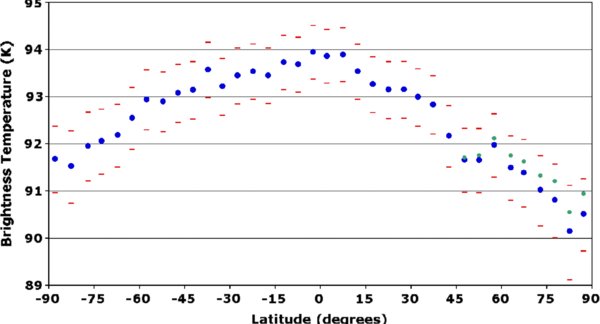
Figure 1. Titan surface brightness temperatures mapped in latitude. Radiances were measured in a 15 cm−1 spectral channel centered at 530 cm−1 and averaged over all longitudes in 5° latitude bins. Each value shown is the average within its latitude bin. Averaged radiances (blue) were corrected for atmospheric opacity, both emission and absorption, and converted to brightness temperature. Values in green include a possible increased H2 opacity in the north reported recently by Courtin et al. (2008). Errors (red) were determined from the number of measurements in each average together with the overall instrumental calibration accuracy. Negative and positive latitudes are south and north, respectively.
Download figure:
Standard image High-resolution image
The latitude dependence of the surface brightness temperature is described by the function

with A = 86.1, B = 7.5, C = 0.0102, and D = 10. The temperature is in kelvin, the latitude is in degrees, and the argument of the cosine is in radians. Even though the highest temperatures are at the equator, the overall distribution described by Equation (1) has a maximum at 10°S. The temperatures decrease toward both poles, reaching 90.5 ± 0.8 K at 87°N and 91.7 ± 0.7 K at 88°S. Courtin et al. (2008) recently reported a possible enhancement in H2 mole fraction at high northern latitudes; when we include this variation by gradually increasing H2 by a factor of 2 between 40°N and 90°N, the coefficients become A = 85.8, B = 7.8, C = 0.0097, and D = 8. The brightness temperatures adjusted for this H2 latitude variation are also shown in the figure.
The north and south polar temperatures are 3 and 2 K below the equatorial temperatures. Our results are consistent with those from the Voyager 1 Infrared Interferometer Spectrometer (IRIS), but have more complete latitude coverage and extend to higher latitudes (Flasar et al. 1981; Samuelson et al. 1997; Courtin & Kim 2002). IRIS saw the ∼2 K decrease near 60°S and 60°N, but did not see the north–south asymmetry, perhaps because it arrived seasonally later than CIRS, near vernal equinox. We agree with the 2.2 cm radar surface radiometry of Janssen et al. (2008) who find a gradual falloff toward the poles of 2 ± 0.8 K. By adopting a peak physical temperature of the equatorial dunes of 93.6 K, they find that the northern lakes have a temperature of 90.5 K, similar to our northernmost zonally averaged values. Cassini radio occultations at several latitudes between 74°S and 73°N give near-surface tropospheric temperatures that are lower by 1–1.5 K in the north (Flasar et al. 2007). In the CIRS observations, the region of large lake formation above 70°N (Stofan et al. 2007; Mitri et al. 2007) has a temperature more than 2 K lower than at the equator. Beyond 70°S, where Ontario Lacus (Turtle et al. 2008) and smaller lakelike features are located, the temperature is more than 1 K lower than at the equator.
Depressed polar temperatures are conducive to lake formation and may explain the larger lake area in the colder north. The saturation vapor pressures of methane and ethane in Titan's atmosphere depend exponentially on temperature. Our observed 3 K drop between equator and north pole implies a 30% decrease in methane saturation vapor pressure and relative humidity, while our observed 1 K between south and north poles corresponds to a 15% difference. For ethane the saturation vapor pressure at the north pole is half that at the equator and the difference from south to north is 25%. Thus, a significant increase in a surface liquid formation rate can be expected at the higher latitudes, especially in the north. The triple-point temperatures for both methane and ethane (90.6 and 89.9 K, respectively) are near the north pole temperature, thereby admitting the possibility of vapor, solid, and liquid coexisting at the surface.
Equator-to-pole differences as large as 2–3 K have typically been difficult to produce in general circulation models (Tokano et al. 1999; Hourdin et al. 1995), although they may be explained by maximum entropy (Lorenz et al. 2001). Furthermore, since the thermal time constant of the troposphere greatly exceeds a Titan year (Tokano et al. 1999; Smith et al. 1981), a north–south temperature asymmetry might be surprising. However, the effective thermal inertia of the surface over an annual cycle is probably much smaller than that of the troposphere (Tokano 2005), and enough sunlight reaches the surface (∼10%; McKay et al. 1991) that seasonal variations in surface temperature are expected. Our observed asymmetry implies that the surface is seasonally heated and that the temperature maximum at 10°S is consistent with late southern summer. Tokano (2007) predicts that near vernal equinox, the warmest latitude close to the surface is at 10°S–30°S, which is roughly confirmed by our results. The temperature distribution in the stratosphere at ∼1 mbar, where seasonal insolation dominates, has been found by both Cassini and Voyager to be shifted the south (Achterberg et al. 2008; Flasar & Conrath 1990; Coustenis & Bézard 1995).
As the temperature distribution shifts northward during Cassini's extended mission, seasonal effects may become apparent. Our preliminary results suggest that the lower stratosphere is cooling in the south and warming in the north as Titan transitions toward northern spring. However, it is too early to discern whether there are temperature trends in the troposphere or at the surface. Seasonal changes of meridional temperatures are expected to give rise to alternating dune-forming winds (Radebaugh et al. 2008) and may help explain the latitudes of cloud formation. As the south transitions to winter Cassini may see the southern lakes grow and the northern lakes diminish. Variations in surface temperature affect the methane mole fraction in the lower atmosphere (Kouvaris & Flasar 1991) and can provide evidence of surface composition and structure (Tokano 2005).
We have looked for local variations in surface temperature with longitude near the equator. Radiative modeling implies that a 10% decrease in albedo can cause a 1 K temperature increase at the surface (Lorenz et al. 1999). Surface altitude might also cause temperature differences given the ∼1 K km−1 adiabatic lapse rate, although Titan's low-relief surface would generally keep these at <1 K. Janssen et al. (2008) present 2.2 cm surface brightness temperature maps showing morphology that matches well with features in optical images (Porco et al. 2005). At our spatial resolution, we should see variations on a scale of the larger features in their maps. We do consistently measure a ∼1 K higher temperature in the vicinity of Belet, a dark equatorial region near 270 W. However, elsewhere near the equator where we have good coverage, we generally find uniformity to within ± 0.5 K. Further data collection will help determine whether two-dimensional temperature maps can be constructed at 530 cm−1.
We acknowledge support from NASA's Cassini mission and Cassini Data Analysis Program. We appreciate helpful discussions with R. Lorenz, M. Janssen, and B. Bézard relating their work to our observations.