


ABSTRACT
We explore the "pre-flare" behavior of the corona in a three-day period building up to an X-class flare on 2006 December 13 by analyzing EUV spectral profiles from the Hinode EUV Imaging Spectrometer (EIS) instrument. We found an increase in the coronal spectral line widths, beginning after the time of saturation of the injected helicity as measured by Magara & Tsuneta. In addition, this increase in line widths (indicating nonthermal motions) starts before any eruptive activity occurs. The Hinode EIS has the sensitivity to measure changes in the buildup to a flare many hours before the flare begins.
Export citation and abstract BibTeX RIS
1. INTRODUCTION
The source of energy for flares is believed to come from a nonpotential magnetic field. One source of this nonpotential energy is flux emergence, which is, for example, observed by Kurokawa et al. (2002) to precede large solar flares. Wang (1992) studied vector magnetic fields for approximately 11 hr before a large flare, and found that magnetic shear is built up through a combination of shear motion and interaction between two opposite polarities. Intermittency of the magnetic field has also been noted starting 30 minutes before flares by Abramenko et al. (2003). The pre-flare behavior in the corona itself has been analyzed in different ways: the excess line width in coronal emission lines has been seen to reach a peak early in the flare with a magnitude of around 200 km s−1 (e.g., Doschek et al. 1980). Harra et al. (2001) found the excess broadening to rise tens of minutes before the flare began, indicating potential pre-flare turbulence that may be related to the trigger mechanism. The excess line width is either due to plasma turbulence or to a distribution of flows. Furthermore, Warren & Warshall (2001) found that the energy release in the pre-flare phase occurs in a different location than in the impulsive phase, suggesting that conditions for a flare may need to be achieved in many places within the source region.
The large X-class flare observed on 2006 December 13 was well observed by the Hinode spacecraft. Kubo et al. (2007) analyzed the photospheric magnetic fields for several days before the flare. The flare occurred at the region where the original sunspot, which had a negative polarity, interacted with an emerging new sunspot with a positive polarity. A day before the flare occurred, bright chromospheric loops appeared around the inversion line between the two sunspots. The inversion line showed a change in the shape at the flare site 8 hr before the flare began. There was also a change in the azimuth angle of the magnetic field of around 90°. The changes responding to the emergence and rotation of the new sunspot have a measurable impact in the corona. Su et al. (2007) analyzed the X-ray images from the X-Ray Telescope (XRT) from December 10 to December 14 to determine the changes in the corona. They found that as the new sunspot emerged the coronal loops were lying perpendicular to the inversion line. However, 12 hr before the flare the coronal loops were lying parallel to the inversion line in a highly sheared formation. There were two large flares that occurred on December 13 and 14, and in both cases part of the sheared core erupted forming a coronal mass ejection (CME) and part of it stayed behind. Abramenko et al. (2008) investigated the intermittency in both the photosphere and the corona building up to X-class flares. They found that peak of the photospheric intermittency occurred 1.3 days before the flare. The coronal intermittency reached a peak after the photospheric intermittency. The injection rate of magnetic helicity was studied for this active region by Magara & Tsuneta (2008), and it was found to reach a peak around 24 hr before the large flare on December 13 occurred. They suggest that the peak is reached after the axis of a flux tube emerges at the photosphere, with subsequent flux emergence therefore being weaker. In this Letter, we investigate the response of the corona to the helicity injection, in particular in terms of the coronal emission line widths.
2. OBSERVATIONS
The data presented in this paper were collected over the period 2006 December 9–13 by the three scientific instruments on board the Hinode spacecraft Kosugi et al. (2007). The EIS instrument, described by Culhane et al. (2007), is a scanning slit spectrometer observing in two wavebands in the EUV: 170–210 Å and 250–290 Å. The spectral resolution is equivalent to approximately 34 km s−1 pixel −1 for the 195 Å emission line, which allows velocity measurements of a few km s−1. The temperature coverage ranges from log T = 4.7 to 7.3 with a spatial resolution of approximately 2''.
We analyze a total of 16 1'' and 2'' slit raster scans from December 9 to 12 in order to track the changes in the line widths and Doppler shifts. The rasters take from about 2 hr to more than 4 hr to construct, and are built up by scanning from west to east. The time given hereafter for each observation is the start time of the observation. We concentrated on the very strong Fe xii 195 Å emission line, and carried out Gaussian fits to this line in each raster scan. Figure 1 shows typical emission line profiles with the Gaussian fits overlaid. This was carried out for each pixel in each raster, resulting in images of the line width and Doppler velocity. The line width measurements were converted into nonthermal velocity by removing the instrumental width and the thermal width. We made use of the Solarsoft routine eis_width2velocity within the EIS software tree. This uses the equation

where vt is the thermal velocity, FWHM is the full width at half maximum of each line profile, λ is the wavelength of the peak of the emission line, c is the speed of light, vnt is the nonthermal velocity, and instrfwhm is the instrumental width.
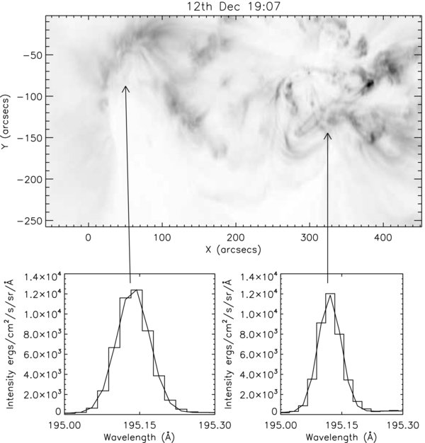
Figure 1. Top image is the Fe xii intensity image on December 12 starting at 19:07 UT. Two sample spectra are shown below. The histogram shows the original data, and the solid line shows the Gaussian fit. The example on the left shows an FWHM of 0.103 Å and on the right shows an FWHM of 0.063 Å. We applied the same fit to all the spectra in all the rasters.
Download figure:
Standard image High-resolution imageThe instrumental width was determined by making use of a joint observing campaign between the Norikura ground-based observatory in Japan and the Hinode spacecraft. The Norikura data were from a high dispersion spectrograph attached to a coronagraph. In order to determine the instrumental width of Fe xii at 195.12 Å, a comparison is made with the Fe x 6374 Å ground-based observation. The instrumental width of Fe x at 195.40 Å is essentially equivalent to that of Fe xii at 195.12 Å because of a gradual change as a function of wavelength. The instrumental width of Fe x at 195.40 Å can be estimated from comparison with line spectra of Fe x 6374 Å in which the instrumental width is known. This value (0.056–0.06 Å) is similar to the value used by Doschek et al. (2007) (0.056 Å). In addition, the Fe xii 195 Å line width is slightly larger than the other Fe xii lines (see Brown et al. 2007). The correction factor of this is assumed to be 2.605 mÅ (see Doschek et al. 2007).
The largest statistical error on the nonthermal velocity is 5 km s−1. The field of view for each raster is slightly different: at least half of the core of the active region is always observed, but the extended loops to the east of the active region are not always in the field of view. In this Letter, we concentrate on the line width measurements, although it is noted that Doppler velocity follows similar behavior, with the largest line widths associated with the largest Doppler velocities. The Hinode Solar Optical Telescope (SOT) Tsuneta et al. (2008) data presented here have previously been analyzed by Magara & Tsuneta (2008).
3. RESULTS
Figure 2 shows how the (hot) coronal loops gradually change following the emergence and rotation of the southerly sunspot. The structure is clearly different between December 9 and December 12. The EIS field of view was not centered on the core of the active region, allowing us to clearly observe the surrounding plasma. In the third EIS raster shown there is a dramatic reduction in the intensity of the corona to the east of the active region core. This appears to be related to an eruption that was seen in the XRT at ≈ 16:40 UT on December 12 (for more details, see Sterling et al. 2009).
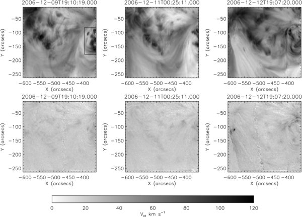
Figure 2. Top row: the EIS Fe xii images on December 9, 11, and 12 shown in a logarithmic scale. The evolution of the active region is clear, in particular the loss of coronal material by December 12 to the east of the main part of the active region. The black box in the first frame marks the region we define as the active region core in the analysis of the line profiles. Bottom row: the nonthermal velocities at the same times with the velocity scale ranging from 0 to 120 km s−1.
Download figure:
Standard image High-resolution imageAs discussed, we determined the line width measurements of each of the EIS rasters analyzed. Figure 2 shows the nonthermal velocity measurements for Fe xii along with the intensity image. Previously, many line width measurements in the corona had either no spatial information (e.g., Yohkoh BCS; Culhane et al. 1991) or did not have the spectral resolution to discriminate small changes in the coronal line widths. The Hinode EIS has both good spatial and spectral resolution, allowing a detailed study of the buildup phase to the large flare. The nonthermal velocity in the core of the active region begins to increase after 21:50 UT on December 11 and before 12:00 UT on December 12. The last pre-flare EIS data (the third image shown in Figure 2 starting at 19:07 UT and ending at 23:46 UT on December 12) shows very large nonthermal velocities. The largest nonthermal velocities are observed far from the flare core (nearly 200'' away). Indeed, in the final pre-flare data, these are the strongest line widths observed in the entire data set. Since not all rasters covered this region to the east of the core, an increase in nonthermal velocity may have occurred in the early part of December 12, but would have remained undetected. However, it is very clear that before the large flare occurred there were large-scale changes occurring in the active region and its surroundings.
We now investigate the nonthermal velocity distribution. Figure 3 shows histograms of the line width observed in each raster between December 9, 19:10 UT and December 12, 19:07 UT. This shows that there is a high nonthermal velocity "tail" to the distribution. We took the median of the nonthermal velocity values above the 95th percentile. These are illustrated in Figure 4 along with the change in helicity with time determined by Magara & Tsuneta (2008). A key point is that the helicity reaches its saturation point before any part of the region experiences significant increases in nonthermal line width. In other words, with the EIS, we observe some dramatic changes in the corona after the peak of the helicity injection rate.

Figure 3. Histograms of the nonthermal velocity (vnt) for each EIS raster from December 9 to 12. The y-axes show the number of pixels in the raster at each measurement of the nonthermal velocity. The top plot shows the nonthermal velocity measurements for the entire EIS field of view. The lower plot shows the nonthermal velocity measurements for only the core of the active region. The time evolution is shown with the earliest nonthermal velocity histogram shown as lighter gray and the later ones as darker. We will concentrate on the tail of the nonthermal velocity histograms to track the behavior of the largest nonthermal velocity with time. It is clear that there the nonthermal velocity is increasing close to the X-class flare on December 13.
Download figure:
Standard image High-resolution image
Figure 4. Top panel shows the GOES X-ray low-energy channel lightcurve from December 9 to 13, including three peaks toward the end of the plotted data, culminating in an X3.4 class flare. The lower plot shows the helicity injection rate as a function of time (dH/dt), as calculated by Magara & Tsuneta (2008), shown as asterisks with values given on the right vertical axis. dH/dt is normalized by 1036 Mx2 s−1. Additionally, we plot the median of the top 95th percentile of nonthermal velocities seen using EIS for the "core" active region area shown by the white box in Figure 2. This is plotted with respect to the left vertical axis. The length of each bar reflects the length of time which EIS took to raster its slit across the respective areas. We note that on December 12 the core nonthermal velocity tail increased to a level above the general fluctuation, before any of the three large peaks seen in GOES X-rays. The vertical black dotted line denotes the time of the third EIS measurement in this trend.
Download figure:
Standard image High-resolution image
4. DISCUSSION
Measurements of excess line widths have been made over the years and it has been well observed that the nonthermal velocity will reach high values before the flare start (e.g., Doschek et al. 1980). In this example we observe changes in the nonthermal velocity hours before the flare occurs. This may be a product of emissivity, sensitivity, and resolution, since the absence of such detections in the EUV until now suggests that the EIS's resolution and sensitivity allow us to see such a phenomenon clearly.
The chronology of changes in the active region are summarized below:
- 1.December 11, 18:00: peak in the spatial intermittency of the photospheric magnetic field. Abramenko et al. (2008) observe a peak in the intermittency of the magnetic field, indicating a corresponding rise in turbulence at this time. The intermittency can be considered as a measure of the complexity of the magnetic field.
- 2.December 11, 20:00: peak in helicity injection rate. The helicity measurements for this event carried out by Magara & Tsuneta (2008) suggest that at the peak of the helicity injection rate, a current sheet could be formed below the axis of an emerging flux tube.
- 3.December 12 after 00:00: chromospheric loops form. These were found by Kubo et al. (2007) close to the inversion line, perhaps indicating low-lying reconnection.
- 4.December 12 after 01:00: a rise in coronal intermittency. This was measured by Abramenko et al. (2008).
- 5.December 12 before 12:00: rise in the coronal nonthermal velocity. This occurs in the core of the active region.
- 6.December 12, 12:43: X-ray loops show high shear. The loops are now all lying parallel to the inversion line (Su et al. 2007).
- 7.December 12, 16:40: small pre-X-flare eruption seen in the XRT.
- 8.December 12 after 19:00: the nonthermal velocity of the large-scale structure to the east of the active region increases.
- 9.December 12, 23:00: second pre-X-flare eruption seen in the XRT.
- 10.December 13, 02:00: X-flare and large-scale eruption begins.
The chronology of events shows changes in the photosphere, followed by changes in the chromosphere and then the corona, finally inducing the large X-class flare. After the saturation of helicity observed in the photosphere, the magnetic field in the upper atmosphere continues to expand, which may form a current sheet above the solar surface (see Figure 7 of Magara & Tsuneta 2008). The saturation of photospheric evolution is necessary for forming a current sheet, because, in this case, the photospheric field is in a state of being "line-tied," which causes the stretching of field lines to form a current sheet. The flux emerges and reaches a high enough altitude to first interact with the chromosphere and then the surrounding corona. The region to the east of the active region is involved in eruptions before the flare. Indeed, this is the location where Imada et al. (2007) measured large blue-shifted plasma following the flare. The region of the largest line width before the flare on December 13 occurred was also the position of largest blue shift following the flare on December 14 (Harra et al. 2007) and the location of the strong "EIT dimmings," indicating the source of the CME.
There are a number of small flares occurring, particularly on December 11 reaching the "C-class" level in GOES before the main flare on December 13. On analysis of the XRT data, these events stay confined to the active region core. As discussed, by December 12 the activity is much more extended outside of the active region. These large-scale loops are clearly important in both the flare initiation mechanism and in the formation of the CME.
In summary, the EIS allows a measurement of changes in the spectral line width hours before the flare began and that this occurs after the helicity injection rate has peaked. In the active region core this increases over a period of 12 hr until the X-class flare begins.
Hinode is a Japanese mission developed and launched by ISAS/JAXA, collaborating with NAOJ as a domestic partner, NASA and STFC (UK) as international partners. Scientific operation of the Hinode mission is conducted by the Hinode science team organized at ISAS/JAXA. This team mainly consists of scientists from institutes in the partner countries. Support for the post-launch operation is provided by JAXA and NAOJ (Japan), STFC (UK), NASA (USA), ESA, and NSC (Norway). G.A.D. is supported by funds from the NASA Hinode program and the NRL 6.1 basic research program.