

Abstract
Methane emissions from small freshwater ecosystems represent one of the largest components of uncertainty in the global methane budget. While these systems are known to produce large amounts of methane relative to their size, quantifying the timing, magnitude, and spatial extent of their emissions remains challenging. We begin to address this challenge in seasonally inundated forested mineral soil wetlands by (1) measuring wetland methane fluxes and hydrologic regime across both inundated and non-inundated soils, (2) characterizing how wetland hydrologic regime impacts the spatial extent of methane emission source areas, and (3) modeling average daily wetland-scale flux rates using four different upscaling techniques. Our results show that inundation extent and duration, but not frequency or depth, were major drivers of wetland methane emissions. Moreover, we found that methane fluxes were best described by the direction of water level change (i.e. rising or falling), where emissions were generally higher when water levels were falling. Once soils were inundated, subsequent changes in water level did not explain observed variability of methane concentrations in standing water. Finally, our spatial modeling suggests that representing inundation and associated methane source areas is a critical step in estimating local to regional scale methane emissions. Intermittently inundated soils alternated between being sources and sinks of methane depending on water level, soil moisture, and the direction of water level change. These results demonstrate that quantifying the hydrologic regime of seasonally inundated forested freshwater wetlands enables a more accurate estimation of methane emissions.
Export citation and abstract BibTeX RIS
1. Introduction
Methane emissions from small freshwater ecosystems such as ponds and forested wetlands represent one of the largest components of uncertainty in the global methane budget. Inventory-based estimates of freshwater methane emissions are higher than expected when compared to top-down models based on atmospheric observations [1]. In part, this discrepancy stems from uncertainty in quantifying methane emissions from mineral soil wetlands, and more specifically, identifying source areas of methane fluxes across intermittently inundated soils. Studies show conflicting reports on how water level variability and wet–dry cycles influence methane fluxes, and it is unclear whether intermittently inundated mineral soils are significant sources of methane [2, 3]. While diurnal variability [4], trophic status [5], the spatial representation of wetland areas [6, 7], and within-lake heterogeneity [8] may explain some of the discrepancy, the potential importance of variable wetland inundation is undetermined.
Methane fluxes are highly variable in freshwater ecosystems and environmental controls on production, consumption, and transport are poorly constrained [9, 10]. Variability in wetland hydrologic conditions, or the wetland hydrologic regime, is a dominant control of methane emissions [11, 12] but its effects are difficult to separate from those of temperature, vegetation, and disturbance history because in wetlands these variables can co-vary and have multiple hierarchical and interactive effects [13–19].
Complex and non-linear relationships between hydrologic and biogeochemical processes in wetlands make it challenging to develop predictive relationships between hydrologic variables and wetland-scale methane emissions. The traditional relationship between water table and emissions is based on assumed separation of an anoxic zone of net production (below the water table) from an oxic zone of net consumption (above the water table) [20]. However, numerous complications have been identified that are hard to account for with this simplification. First, production is not limited to below the water table because methanogenesis can occur in anoxic microsites in otherwise oxygenated soil above the water table [21–24]. Second, methanotrophy is not limited to the oxic portion of the soil column in the presence of anaerobic methane oxidizers [25, 26]. Time series of flux measurements have also shown temporal lags between changes in water level and changes in methane emissions [27, 28], and lateral concentration gradients caused by plants can spatially separate areas of production from emissions [29]. Finally, in wetlands with surface inundation, transport and reaction processes in surface water can modulate the amount of methane that reaches the atmosphere [30–32]. Some authors have suggested that deeper surface inundation should result in more methane oxidation because of slow gas diffusion through water [11, 33]. Although there is often less dissolved methane in deep (>6 m) compared to shallow water of lakes [34], this pattern has not been demonstrated for shallower wetlands.
In addition to hydrologic drivers of methane production and consumption, the assumptions about methane cycling in different land cover types may contribute large uncertainty to emission estimates. Land cover classifications of wetlands generally exclude inundated mineral soils [35]. This omission means that flooded areas of mineral soil in forests, which can be locally or intermittently high methane sources [36–39], do not typically register as methane producing areas in models [6]. Instead, mineral forest soils are considered the largest terrestrial sink for atmospheric methane [40]. Among the most well-studied type of wetlands—peatlands—methane fluxes are generally negative when the water table drops to ∼10 cm below the peat surface (e.g. [41]), but it is unclear how intermittent flooding affects methane fluxes in fundamentally different wetland types [16]. The transition between methane sources and sinks in temperate forested wetlands may be a dynamic zone controlled by soil moisture [36, 37, 42]; however, no studies have explicitly attempted to quantify how this boundary varies in time or space.
Treating intermittently or seasonally flooded mineral soils as potential sources of even very small methane fluxes has large implications in emission models because of how expansive this area is globally [43–46]. Filling this gap in our understanding of methane emissions is important for informing earth system models that rely on observations of surface water for determining areal extent of emissions [47, 48]. Improved representation of inundation dynamics in forested wetlands for methane emission models is especially warranted given that forested wetlands experienced the largest change in area of any wetland type in the United States between 2004 and 2009 [49], and the area of soils experiencing periodic drying or inundation cycles may be expanding due to increasing variability in precipitation rates and development-induced land cover changes [50].
Here, we assessed the role of hydrologic variability on methane emissions in freshwater forested mineral soil wetlands by (1) quantifying the relationship between water level above (+) and below (−) the soil surface and methane flux rates throughout a water year, (2) characterizing the spatial extent of methane emission source areas for seasonally dynamic wetlands, and (3) comparing wetland-scale flux estimates using different upscaling techniques.
2. Methods
We measured methane fluxes monthly across inundation gradients in six forested wetlands over one water year and quantified the hydrologic regime of each wetland from water levels monitored at multiple points within each wetland. The relationship between water level and methane flux rates, and the extent of methane emission source areas were evaluated with statistical models. Water level time series and average flux rates from inundated and non-inundated zones were used to estimate wetland-scale emissions under contrasting assumptions regarding methane source area dynamics.
2.1. Study area and hydrologic setting
We identified six forested wetlands in the mid-Atlantic Coastal Plain characterized by seasonal changes in water level and minimal emergent vegetation. Sites were in the Upper Choptank River watershed on the Delmarva peninsula which drains to Chesapeake Bay (figure 1). This low-gradient watershed comprises 60% cropland, 20% woody wetland, 12% forest, and <5% developed land [51]. Forests contain a patchwork of seasonally flooded area, complex microtopography, sphagnum, narrow ditches from a legacy of drainage, and abundant depressional wetlands called Delmarva bays [52]. These features range in size from 0.5 to 0.7 ha [53, 54] and include large open canopy areas as well as more numerous small forested depressions [55, 56]; the latter of which are the focus for this study. Depressions have a seasonal hydrologic regime driven by evapotranspiration from a highly permeable shallow groundwater aquifer. They are inundated up to ∼150 cm above the soil during late fall and winter, then, depending on rainfall and landscape position, may lose all surface water as the regional water table drops throughout the growing season [57]. Soils at our study sites are poorly or very poorly drained, with either loamy sand, mucky loam, or moderately decomposed plant material comprising the top 5 cm (table 1 [58]).

Figure 1. Locations of six forested wetland study sites (W1-6) within the Upper Choptank River watershed (Tuckahoe Creek HUC 0206000501 and Watts Creek-Choptank River HUC 0206000502) and hydrologic regime classifications of National Wetland Inventory freshwater wetlands.
Download figure:
Standard image High-resolution imageTable 1. Properties of wetland study sites. Values are mean ± standard deviation and (range).
| Max area inundated (m2) | Inundation index | Water level (m) | NRCS soil type | Soil bulk density (g m-3) | Dissolved CH4 (µmol L−1) | DOC (mg L−1) | Inundated flux rate (mmol m−2 d−1) | Non-inundation source flux rate (mmol m−2 d−1) | Non-inundated sink flux rate (mmol m−2 d−1) | Non-inundated source zone buffer width (m) | Scaling correction factor | |
|---|---|---|---|---|---|---|---|---|---|---|---|---|
| W1 | 1920 | 0.56 | 0.39 (0–0.71) | Hammonton-Fallsington-Corsica | 0.070 | 22.0 ± 23 (1.1–58.3) | 34.8 | 2.97 ± 3.1 (n =10) | 0.40 ± 0.90 (n = 16) | −0.003 ± 0.002 (n = 28) | 5.4 ± 4.7 | 0.62 |
| W2 | 597 | 0.58 | 0.63 (0.17–1.09) | Hammonton-Fallsington-Corsica | 0.448 | 7.6 ± 9 (0.5–24.0) | 34.6 | 1.02 ± 1.2 (n = 9) | 0.16 ± 0.48 (n = 10) | −0.004 ± 0.004 (n = 29) | 1.7 ± 2.7 | 0.61 |
| W3 | 2065 | 0.56 | 0.61 (0.22–0.93) | Corsica mucky loam | 0.239 | 16.8 ± 21 (5.7–71.1) | 40.9 | 2.27 ± 2.9 (n = 9) | 0.08 ± 0.16 (n = 15) | −0.004 ± 0.003 (n = 27) | 2.9 ± 2.7 | 0.57 |
| W4 | 1639 | 0.72 | 0.60 (0.17–1.03) | Hammonton-Fallsington-Corsica | 0.267 | 2.8 ± 2.6 (0.8–9.5) | 24.8 | 0.38 ± 0.35 (n =10) | 0.07 ± 0.12 (n = 9) | −0.003 ± 0.001 (n = 37) | 1.8 ± 1.8 | 0.74 |
| W5 | 1710 | 0.57 | 0.40 (0.04–0.70) | Lenni loam | 0.267 | 3.1 ± 1.9 (1.2–6.9) | 29.7 | 0.41 ± 0.26 (n = 8) | 0.18 ± 0.60 (n = 19) | −0.003 ± 0.001 (n = 29) | 6.3 ± 4.2 | 0.69 |
| W6 | 380 | 0.60 | 0.34 (0.15–0.46) | Hammonton-Fallsington-Corsica | 0.184 | 14.7 ± 9.8 (3.6–35.8) | 27.0 | 1.98 ± 1.3 (n = 8) | 0.37 ± 0.92 (n = 13) | −0.003 ± 0.003 (n = 13) | 2.2 ± 2 | 0.63 |
Methane measurements were made near each wetland center and at five evenly spaced locations along wetland to upland transects (figure 2). This captured both temporal and spatial variations in hydrologic conditions, which we quantified using metrics described below and in table S1 (available online at stacks.iop.org/ERL/16/084016/mmedia). Throughout, water level refers to the position of the wetland water table relative to the soil surface: positive values indicate inundation and negative values indicate soils were not inundated. The broader water table surrounding a wetland is referred to as the groundwater table [57]. While the timing and seasonality of precipitation and evapotranspiration drive temporal variation in hydrologic conditions [59], wetland morphometry drives spatial gradients in hydrologic conditions (i.e. both inundation duration and soil moisture decrease along each transect from wetland center to upland).
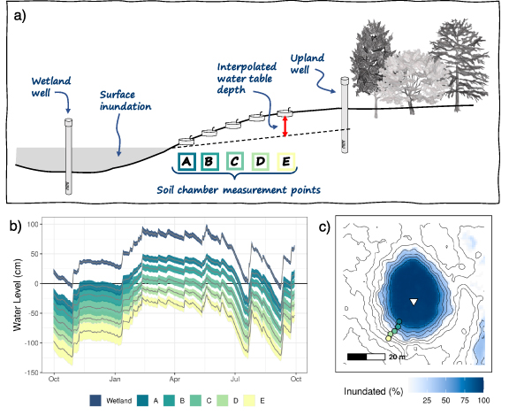
Figure 2. (a) Site design showing relative locations of wetland and upland surface water wells and soil flux chambers (not to scale); (b) average (±sd) water level hydrographs at wetland well and chamber measurement points; (c) topography, modeled inundation frequency, and locations of measurement points (dots) and wetland well (triangle) at one of the six wetland sites. Contour lines show 20 cm elevation increments from the lowest point of the wetland.
Download figure:
Standard image High-resolution imageWe quantified hydrologic variation using a combination of water level, elevation surveys, and a 1 m digital elevation model (DEM [59]). We estimated inundation extent at each wetland using daily water level and the DEM [60], and estimated water level at soil chamber points by interpolating between the inundation boundary and water level at the upland end of each transect (figure 2(a)) [61]. Using each of these daily water level time series, we derived time series of the magnitude and direction of water level change over the previous 1–7 d (WL1–7 and ΔWL1–7). We then summarized hydrologic variability over the water year at each chamber location by calculating the average and range in water levels, and the frequency and maximum duration of periods with negative or positive water levels. We summarized hydrologic variability at the wetland scale using surface water extent time series to calculate the cumulative proportion of area inundated throughout the year ('inundation index').
2.2. Methane flux measurements
Methane emissions were calculated using monthly measurements at each wetland across the 2018 water year. Different techniques were used to quantify diffusive fluxes from inundated and non-inundated zones of each wetland (see details in Text S1). For inundated areas we used the turbulent boundary layer method with replicate measurements of dissolved gas concentrations sampled near wetland centers and a gas exchange model for wind-sheltered water bodies [62, 63]. Fluxes from non-inundated areas were calculated from 24 h incubations of 1–2 l static flux chambers installed along wetland transects (figure 2) [64]. Although monthly sampling may not adequately capture the full range of variability in emissions, our intention was to assess the extent to which the seasonal hydrology might explain observed variability in fluxes. This design allowed for sampling all study wetlands over a 2 d period. The relationship between hydrologic metrics (table S1) and methane fluxes was evaluated using generalized linear mixed effects models using wetland site as a random effect. Stepwise regression was used to evaluate fixed effects, including air and soil temperature, and to remove highly correlated effects; model fit was evaluated using AIC and marginal R2 values. The magnitude of flux rates from inundated and non-inundated source and sink areas were compared using Wilcoxon signed rank tests.
2.3. Spatial extent of methane emissions
To analyze the lateral boundary between net methane sources and sinks, we assessed whether the source area expanded and contracted over time in accordance with hydrologic conditions, or alternatively, if the transition was a relatively fixed location at each wetland. To do this, we used logistic mixed effect models to evaluate whether metrics representing point-scale hydrology (described above) or location were stronger predictors of whether a measured flux was positive or negative.
2.4. Wetland-scale flux models
To compare approaches for upscaling to the wetland scale, we calculated emissions for each wetland using four simple models with different assumptions regarding methane source areas (figure 3, table 2). Wetlands were modeled as three concentric zones with differing flux rates: a central inundated 'source' zone with positive emissions, a surrounding non-inundated source zone, and an outer non-inundated 'sink' zone with methane uptake. The models vary based on which zones are included in calculating emissions, and whether the size of the inundated zone varied. Model I assumed emissions are from a fixed inundated area throughout the year (hereafter, fixed-area model). Model II calculated fluxes from inundated area time series, with no emissions from non-inundated zones (variable-area, excluding non-inundated). Model III included emissions from both inundated and non-inundated source areas (variable-area, including all sources), and Model IV calculated net emissions from all three zones (variable-area, sources and sinks). Each model was run 1000 times for each wetland at the daily time scale for one year, with inputs derived from the field measurements described above. Wetland-specific water level time series were fixed, but daily inputs of both non-inundated source zone buffer widths and flux rates for each of the three emission zones were sampled from distributions fit to the relevant observations averaged for each site.
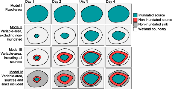
Figure 3. Overview of the four scaling models used to estimate wetland flux rates. Daily wetland-scale emissions are calculated from areal extent and flux rates from 1, 2, or 3 wetland zones. Inundated area used in variable area models (II, III, and IV) is determined from mean daily water level. Non-inundated source area (Models III and IV) is calculated as a buffer around the inundated area with a width sampled from a distribution of wetland-specific observations (see section 2.4). The area of the non-inundated sink zone (only in Model IV) was calculated as the difference between the wetland boundary and the combined area of the inundated and non-inundated source zones. Flux rates for each of the three zones were sampled from wetland-specific distributions of the relevant measurements.
Download figure:
Standard image High-resolution imageTable 2. Areas represented in each of the four inundation models. See section 2.4 for details. Wetland boundary is defined from the maximum observed inundation extent during the period of study.
| Inundated source zone | Non-inundated source zone | Non-inundated sink zone | |
|---|---|---|---|
| Model I | Wetland boundary | Not included | Not included |
| Model II | Daily surface water extent | Not included | Not included |
| Model III | Daily surface water extent | Daily estimate of buffer surrounding surface water extent | Not included |
| Model IV | Daily surface water extent | Daily estimate of buffer surrounding surface water extent | Remainder between wetland boundary and source zones |
3. Results
3.1. Methane flux rates and water level
Overall, flux rates showed high variability and differed significantly between wetland zones (figure 4; p < 0.001). Inundated zone fluxes averaged 1.36 ± 2.08 mmol m−2 d−1 and non-inundated zone fluxes averaged 0.07 ± 0.4 mmol m−2 d−1. No positive emissions were measured from points with water level −90 cm below the soil surface; however, uptake was measured across a wide range of water levels, including from fully saturated soils. On average, water levels varied a range of 130 cm throughout the year with minimums in late October 2017 and late September 2018 and maximums during March 2018 (figure 2; table 1).
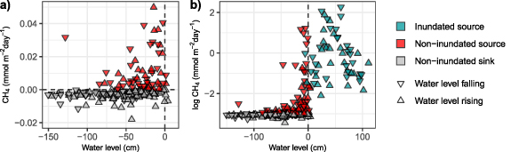
Figure 4. Relationship between water level and methane flux rates. In (a) only fluxes near 0 are shown for greater detail. Points above the horizontal line are positive emissions and points below the line are negative (uptake). In (b) all flux values are shown on a log scale. Points to the left of the vertical line are from non-inundated soils and points to right of the vertical line are measurements from inundated soils.
Download figure:
Standard image High-resolution imageMixed effect models indicated that flux rates from inundated soils were best explained by the direction of water level change (ΔWL1 ; R2 = 0.39) and were not significantly related to water level. These fluxes were ∼55% lower when water levels had risen rather than fallen since the previous day (table 3; figure S2). Water levels were also not a significant predictor of fluxes from non-inundated soils: variability was best explained by soil moisture and the direction of water level change over the previous week (ΔWL7 ; R2 = 0.26). Fluxes from non-inundated soils were approximately 32% lower when the water level had risen rather than fallen over the previous week (i.e. methane fluxes were greater when water level was receding). However, the model for non-inundated soils had low explanatory power and was unable to adequately capture the variance in our observations. Residuals showed consistent underprediction of the largest 10% of measured fluxes (>0.1 mmol m−2 d−1). Dissolved methane concentrations were highly variable and ranged over two orders of magnitude (0.54–71 µmol L−1). This variability was not correlated with water level or temperature, however we observed peaks at all sites in late summer, coincident with the lowest water levels and highest temperatures.
Table 3. Regression parameters for random intercept mixed effect models explaining variability of methane flux rates measured from inundated and non-inundated soils. Wetland site is included as a random effect. ΔWL1 and ΔWL7 are the direction of water level change (increasing or decreasing) over the previous one and seven days respectively.
| Inundated zone | |||
|---|---|---|---|
| Conditional R2 | 0.39 | ||
| Marginal R2 | 0.12 | ||
| Estimate | t | p-Value | |
| Intercept | 0.08 | 0.287 | 0.78 |
| ΔWL1 | −0.81 | −3.149 | <0.005 |
| Non-inundated zone | |||
| Conditional R2 | 0.26 | ||
| Marginal R2 | 0.19 | ||
| Estimate | t | p-Value | |
| Intercept | −3.40 | −28.80 | <0.005 |
| ΔWL7 | −0.30 | −3.77 | <0.005 |
| Water filled pore space | 0.02 | 6.01 | <0.005 |
Average flux rates over the course the year were significantly correlated with metrics summarizing hydrologic variability at each measurement point (figure S1). Median water level (ρ = 0.83, ρ = 0.83, p < 0.05) and duration of inundation (ρ = 0.82, ρ = 0.83, p < 0.05) had strong positive correlations with average log fluxes. Metrics describing hydrologic variability were largely correlated with each other, except for the frequency of dry periods (i.e. when water level <0), which was not correlated with flux rates. Range and standard deviation of water level had weak negative correlations with range and standard deviation of flux rates (ρ ∼ −0.40, p < 0.05).
3.2. Spatial extent of source and sink zones
We observed both methane emissions and uptake over wide and overlapping ranges of hydrologic conditions. Nearly all measurement points transitioned between being methane sources during generally wetter conditions and methane sinks during drier conditions. However, we measured positive fluxes from locations with water levels as low as ∼80 cm below the soil surface and up to ∼8 m outside of the wetland boundary, and occasionally measured negative fluxes from points with fully saturated (but not inundated) soils.
The distinction between source and sink measurements was better explained by variables associated with hydrologic conditions rather to those associated with measurement position. Water level, direction of water level change, and soil moisture together explained 55% of the difference between source and sink measurements, whereas the position of measurement locations only explained 20% (table S2). According to the best fitting model, positive emissions were more likely when water levels had fallen since the previous day, when the water level was above −25 cm, or when soil moisture exceeded ∼70% water filled pore space (figure S3).
3.3. Wetland-scale flux rates
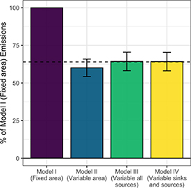
Wetland-scale emissions estimates were the highest using the fixed area model (i.e. assuming no changes in inundation extent), and lowest using the variable-area model that excluded non-inundated regions (figures 5 and S5). Estimates calculated using all sources and sinks were not significantly lower than those using the variable area all sources model. In Model IV, on average 94% of emissions were from the inundated zone. Emissions estimated using variable inundation extents were between 57% and 74% of the emissions calculated under the fixed-area model. This difference was positively correlated with the inundation index (ρ = 0.73, p < 0.001) and negatively correlated with methane flux rates (ρ = −0.69, p < 0.001), meaning the largest discrepancies from the fixed area model were for wetlands with a low inundation and high methane flux rate. Uncertainty was highest for wetlands with the largest variability in inundation zone methane flux rates.
Figure 5. Average difference in annual upscaled wetland emissions calculated using different sets of assumptions regarding inundation dynamics (see section 2.4 and figure 3 for model details). Error bars represent standard deviation across the six study wetlands. Horizontal line at 64% indicates mean of Model IV.
Download figure:
Standard image High-resolution image
4. Discussion
Overall, we found that hydrologic variability—particularly the inundation extent and duration—was an important predictor of wetland-scale methane flux rates from forested mineral soil wetlands. Inundated soils were consistently a source of methane; and much of the variability in these fluxes was explained by direction of water level change, and surprisingly, not water level itself. Intermittently inundated soils alternated between being methane sources and sinks depending on hydrologic conditions. Below we discuss how the wetland hydrologic regime may be controlling methane production and emissions from mineral soil wetlands, and how this variability affects upscaling of freshwater methane emissions from wetland to regional scales.
4.1. Effects of hydrologic variability on methane fluxes
Inundated soils were the dominant source of methane emissions. Standing water had high, but variable concentrations of dissolved methane that were similar in magnitude to concentrations found in other small open water ecosystems (table 4). The observed concentrations exceed values typical of both larger lakes (<2 µmol l−1 [65, 66]) and flowing waters (1.35 ± 5.16 µmol l−1 [67]). Variability was not explained by water level above the soil surface, which suggests that once wetlands are inundated, subsequent changes in water level do not have a strong effect on rates of production and consumption of methane within standing water. Effects of water depth on methane concentrations and fluxes may only occur over a larger range of water levels than we observed (>1.5 m) or over shorter time periods than monthly sampling could capture. This pattern is broadly consistent with findings of a recent global synthesis, showing seasonally averaged emissions sharply increase up to a critical water level above the soil surface, above which there is high variability [68].
Table 4. Reported methane concentrations and fluxes from small open water ecosystems. N is the number of individual systems studied; concentration and flux values are average ± standard deviation and/or range of measurements (low–high) depending on details provided in each study.
| System type | CH4 concentrations (µmol L−1) | CH4 fluxes (mmol m−2 d−1) | N | Reference |
|---|---|---|---|---|
| Forested wetlands/ponds | 27 ± 4.6 (0.4–210) | 10.8 ± 18.5 (0.2–73) | 4 | Kifner et al 2018 [69] |
| 11.3 ± 15.6 (0.54–71) | 0.38–2.97 | 6 | This study | |
| 33.4 (21.0–58.9) | 10.6 ± 0.13 | 6 | Holgerson 2015 [70] | |
| (−0.12–3.36) | 3 | Morse et al 2012 [71] | ||
| Prairie pothole wetlands | 0.2–34.3 | 5.1 (0.30–36.5) | 2 | Martins et al 2017 [72] |
| 6.1–15.7 | 0.7–13.3 | 3 | Bortolotti et al 2016 [73] | |
| (0.1–3.8) | 62 | Baidou et al 2011 [74] | ||
| 0.63 ± 0.05 (−0.06–4.36) | 1 | Bansal et al 2018 [75] | ||
| (0.06–243.10) | 119 | Tangen et al 2015 [76] | ||
| (0.46–22.32) | 88 | Tangen and Bansal [29] | ||
| Agriculture/aquaculture ponds | 2.29–50.48 | 4.56 (2.16–55.68) | 3 | Yang et al 2019 [77] |
| 7.2 ± 1.74 | 77 | Ollivier et al 2019 [78] | ||
| 0.93–87.58 (0.06–338.15) | 22 | Grinham et al 2019 [45] | ||
| 16.43 ± 1.06 | 3 | Yuan et al 2019 [79] | ||
| Urban/stormwater ponds | 1.62 (0.11–20.23) | 1.89 (0.02–10.85) | 40 | Peacock et al 2019 [80] |
| 0.93–36.78 | 7 | Herrero Ortega et al 2019 [81] | ||
| 1.25 ± 18.70 | 1 | van Bergen et al 2019 [82] | ||
| 22.59 (0.45–114.14) | 15 | Gorsky et al 2019 [83] | ||
| Boreal/permafrost thaw ponds | 9 (0.02–47) | 146 | Polishchuk et al 2018 [84] | |
| 3–40 | (6.86–11.2) | 30 | Hamilton et al 1994 [85] | |
| 0.3–6.2 | (0.01–12.8) | 7 | Matveev et al 2016 [86] | |
| 0.04–5.17 | (0.03–5.62) | 52 | Laurion et al 2010 [87] | |
| 24 ± 3 | 9.35 ± 0.27 | 52 | Kuhn et al 2018 [88] | |
| 1.1 | (1.3–2.3) | 1 | Dabrowski et al 2020 [89] | |
| (0.22–0.47) | 2 | Huttunen et al 2002 [90] | ||
| Beaver ponds | (7.1–17.3) | 9.35 | 2 | Yavitt et al 1992 [91] |
| 15.6 (0.06–87.3) | 1 | Yavitt et al 1990 [92] | ||
| (8.66–57.3) | 4 | Bubier et al 1993 [93] | ||
| (0.87–1.0) | 2 | Ford and Naiman 1988 [94] | ||
| 2.3 ± 1.9 | 1 | Weyhenmeyer 1999 [95] | ||
| 5.87 | 1 | Roulet et al 1997 [96] | ||
| 5.8–5.3 (1.12–34.66) | 3 | Lazar et al 2014 [97] |
Because the direction of water level change was a better predictor of flux rates than water level, this may indicate a lagged relationship between water level and methane emissions, as has been found for other freshwater wetlands where water table depth is a major predictor [98]. When soils are unsaturated, alternate electron acceptors such as ferric iron and sulfate may re-oxidize and provide substrate for microbes that use more thermodynamically favorable pathways to then outcompete methanogens [99–101]. Such an effect would suppress methane production after periods of lower water levels and explain why we observed lower methane fluxes during rising rather than falling water levels. Increasing water levels can also reduce the supply of organic substrate for methanogens through dilution and effects to productivity of aquatic vegetation [68]. Additionally, changes in water level relative to the groundwater table could affect lateral transport of dissolved methane into wetland surface water through shallow subsurface flowpaths controlled by hydraulic gradients, especially for mineral soil wetlands with high labile carbon pools. This lateral transport can concentrate methane produced in deeper soil layers of the surrounding wetland catchment, resulting in spatial discontinuities between factors driving methane production (e.g. water level, soil carbon content), oxidation, and emission. Lateral flowpaths are common in wetland-rich landscapes like the Prairie Pothole Region and the Delmarva Peninsula [57, 102].
Average methane fluxes at each measurement point were correlated with metrics summarizing the duration but not frequency of inundation. This aligns with other studies that found large fluxes associated with flooding induced inundation [27, 103] and continuous saturation [11]. The frequency of wetting and drying cycles may be related to methane flux potential in soils [50], but have complex interactions with vegetation and the timing of drying/drainage such as in efforts to mitigate emissions from flooded rice agriculture [104].
The relationship between wetland hydrology regime and methane emissions has implications for total freshwater wetland emissions in the US because recent trends show losses of coastal forested wetlands and gains in wetland types with more stable water levels such as farm ponds and created wetlands on previously drained mineral soil [49, 105]. Our results suggest that this trend could be leading to higher net methane emissions because of increased inundation, however there are also plausible mechanisms for increased frequency of wet-dry cycles in forested wetlands to result in higher emissions.
4.2. Spatial extent of methane uptake and emissions
Fluxes from non-inundated soils transitioned between uptake and emissions depending on hydrologic conditions, and flux rates were only partially explained by soil moisture and the direction of changes in water level. Our findings align with the emerging conceptual framework for peatland soils that a distinct vertical separation between zones of methane production and consumption is unlikely, and that fluxes are mainly controlled by other environmental factors that are linked to hydrologic dynamics in complex ways [23]. This is especially relevant in low-gradient landscapes with shallow groundwater tables where large areas of mineral soil can become inundated (or pass a soil moisture threshold for methane emissions) with even small changes in water levels [43]. Under these circumstances, methane source areas will not be limited strictly to wetland soils. Our results suggest appropriately representing methane source areas in emission models requires improved modeling of hydrologic processes that lead to inundation of small-scale features like topographic depressions and ditches [106].
Methane uptake was not limited to unsaturated soils, but rather occurred under a wide range of hydrologic conditions potentially by different microbial communities. Maietta et al [61] analyzed the microbial community composition from soils collected at the same measurement points used in this study and found methane oxidizers along a wider range of the hydrologic gradient compared to methanogenic archaea. Flux measurements align with results of the microbial community composition, showing there is a capacity for both methanogenesis and methane consumption within and slightly upland of intermittently inundated soils. Although additional factors such as low soil pH may limit net emissions from these systems [107], these results underscore the need for considering both methane consumption and production in wetland emission models in order to accurately predict net fluxes.
4.3. Inundation extent as a proxy for methane source areas
The methane emissions source area of our study sites could reasonably be approximated by a time series of surface water extent because the actual source area included minimal emissions from surrounding non-inundated soils. Areal wetland-scale flux rates were substantially lower (26%–43%) in models that accounted for inundation variability. One way to incorporate this seasonal drying is to use a correction factor when scaling up methane flux rates from similar small water bodies in landscape or regional assessments that do not otherwise quantify hydrologic variability. Similarly, experimental work in Prairie Pothole wetlands [28] and on small water bodies in Australia [45] calls for incorporating hydrologic variability when scaling up flux rates. Our models showed that a reasonable approximation of diffusive emissions would be scaling wetland area by 64%, which surprisingly matches the variability in surface area for the smallest size class water bodies reported by Grinham et al [45]. We account for minimal fluxes from non-inundated zones but inundated zones contributed the overwhelming majority of emissions in our models (83%–99%). Across a long-term dataset of emissions from Prairie Pothole wetlands, Tangen and Bansal [28] also found that continuously wet zones accounted for >85% of cumulative fluxes. Using this correction factor approach relies on a reference wetland boundary, which for Grinham et al [45] was based on analyzing a time series of high-resolution aerial imagery. We determined these areas empirically during our study period, however reliable maps of small water bodies, especially forested wetlands, are rare.
Our study suggests that seasonally inundated forested wetlands are substantial sources of methane at the landscape scale in the Upper Choptank River watershed. Emission estimates from the variable area sources and sink model (IV) indicate an average areal flux rate of at least 1.65 kg m−2 yr−1, which is four orders of magnitude greater than the average methane uptake rate in temperate forest soils [108], even after accounting for a small amount of uptake within the wetland. Across the Upper Choptank River watershed, a third of the land is forest and forested wetlands. Hydrologic classifications in the National Wetlands Inventory suggest that almost 30% of that area is non-riverine freshwater wetlands subject to at least temporary or intermittent flooding (table S3) and therefore potential sources of methane emissions. Improved methods for detecting and modeling surface water dynamics in low relief landscapes will greatly improve our ability to quantify methane emissions from forested wetlands.
5. Conclusions
Understanding controls on methane fluxes in wetlands is needed to account for them properly in earth system models and to predict impacts of changing land cover and climate. We demonstrate that quantifying the hydrologic regime of seasonally inundated forested freshwater wetlands enables a more accurate estimation of their methane emissions. Hydrologic variability helped explain whether methane fluxes were positive or negative, and flux rates were lower during rising rather than falling water levels. Future work should assess the role of methane oxidation in reducing net evasion of methane from wetlands with standing water. We found that intermittently flooded soils transitioned between methane sources and sinks depending on hydrologic conditions; and using spatially explicit models, we found that the majority of methane emissions could be estimated from the inundated portions of these wetlands.
Acknowledgments
We are grateful to The Nature Conservancy for managing and providing access to the land where this study was conducted, to C Maietta for comments on previous drafts, and to A Armstrong, A Kottkamp, and J Greenberg for fieldwork assistance. This work was supported by the National Socio-Environmental Synthesis Center under funding received from the National Science Foundation DBI-1639145.
Data availability statement
The data that support the findings of this study are openly available at the following URL/DOI: https://doi.org/10.5281/zenodo.5032390 [109].