

Abstract
Understanding plant responses to hydrological extremes is critical for projections of the future terrestrial carbon uptake, but much more is known about the impacts of drought than of extreme wet conditions. However, the latter may control ecosystem-scale photosynthesis more strongly than the former in certain regions. Here we take a data-driven, location-based approach to evaluate where wet and dry extremes most affect photosynthesis. By comparing the sensitivity of vegetation greenness during extreme wetness to that during extreme dryness over a 34 year record, we find that regions where the impact of wet extremes dominates are nearly as common as regions where drought impacts dominate. We also demonstrate that the responses of wet-sensitive regions are not uniform and are instead controlled by multiple, often interacting, mechanisms. Given predicted increases in the frequency and intensity of extreme hydrological events with climate change, the consequences of extreme wet conditions on local and global carbon cycling will likely be amplified in future decades.
Export citation and abstract BibTeX RIS

Original content from this work may be used under the terms of the Creative Commons Attribution 4.0 license. Any further distribution of this work must maintain attribution to the author(s) and the title of the work, journal citation and DOI.
1. Introduction
Terrestrial carbon uptake by photosynthesis is strongly influenced by climate (Friedlingstein et al 2006) and its extremes (Reichstein et al 2013). As the climate warms, the hydrological cycle is intensifying (Trenberth 2011), yielding shifts in the regimes of extreme dry and extreme wet events (Seneviratne et al 2012). Droughts are expected to become more intense, spatially extensive, and temporally persistent (Trenberth et al 2014), while an enhancement of extreme wet precipitation has also been both projected (Fischer et al 2013) and observed (Donat et al 2016) on continental to global scales. To reduce uncertainties in future projections of the carbon cycle (Friedlingstein et al 2013), a robust understanding of the feedbacks between extreme hydrological events and terrestrial carbon uptake is crucial.
Because of this, the effects of droughts on growth and photosynthesis have been studied extensively (e.g. Farooq et al 2012, Schwalm et al 2017, Xu et al 2019). However, responses by vegetation to extreme wet events are poorly understood by comparison. One possible contributor to this knowledge gap is the fact that, when globally averaged across the land surface, the impacts of extreme dry events on productivity have been shown to dominate those of extreme wet events (Zscheischler et al 2014). Such globally integrated values, however, may not fully capture the spectrum of relative impacts possible at any given location. Droughts are significantly more spatially coherent and less temporally transient than heavy rainfall events, which may contribute to the greater global impact of the former, regardless of which extreme is more influential in individual regions.
Overall, whether vegetation in any particular place is more sensitive to extreme wet events than to extreme dry events remains unclear. This is a crucial distinction because changes in the behavior of extreme hydrological events are also projected to vary regionally (albeit with high uncertainty (Trenberth 2011)). That is, different regions will experience different trends in extreme precipitation, with some getting wetter and others drier. If hotspots of sensitivity to extreme wet events exist now, their future consequences on local and global carbon cycling could be even more pronounced. Furthermore, understanding how the vulnerability of different regions to hydrological extremes varies may impact conservation or management priorities.
Beyond the importance of extreme wet events on sub-global scales, even the dominant sign of the photosynthesis response under extreme wetness is poorly quantified across the broader land surface. Significant heterogeneity in both sign and magnitude of the vegetation response to extreme wetness has been observed at ecosystem scales (Heisler-White et al 2008, Knapp et al 2008), indicating its dependence on locally- and regionally-specific factors. A multitude of processes can impact the response of vegetation to extreme wet conditions. Some such mechanisms may cause photosynthesis to increase (e.g. by alleviating a moisture limitation or by mitigating heat-related stresses (Li et al 2019)), while others may induce negative effects (e.g. associated with the consequences of partial to complete flooding (Bailey-Serres and Voesenek 2008, Garssen et al 2015)). Because a bottom-up study tracing each process to its impact on carbon uptake is not feasible given the data that is currently available, here we take a top-down approach by first quantifying vegetation responses during extreme wet conditions and then inferring likely mechanisms that explain the observed patterns.
This paper investigates regional variations in the relative impacts of extreme wet events and extreme dry events on vegetation. To do so, average vegetation greenness anomalies (relative to the local climatology) during periods of extremely high moisture were compared to those during periods of extremely low moisture by leveraging 34 years of satellite normalized difference vegetation index (NDVI) data from the Global Inventory Monitoring and Modeling System (GIMMS) alongside combined active and passive soil moisture observations from the European Space Agency Climate Change Initiative (ESA CCI) (see section 2). Although NDVI is a direct measure of spectral reflectance, not photosynthesis (Tucker 1978), it is used here because of its long temporal record, observational nature, and global spatial coverage.
Specifically, in this paper we seek to answer the following questions. (a) Across the vegetated land surface, where is greenness more sensitive to extreme wet events than it is to extreme dry events? (b) What controls the sign of the resulting greenness change during extreme wet events?
2. Methods
2.1. Data selection and processing
Two datasets derived from satellite remote sensing were used to represent vegetation productivity and moisture conditions. These datasets were selected on the basis of their (a) long temporal records (i.e. >30 years), (b) moderate-to-high spatial resolutions, (c) global coverage, and (d) observational nature (i.e. absence of assumptions about vegetation behavior embedded in the datasets).
We used the GIMMS NDVI third generation data product as a proxy for vegetation productivity. The dataset is derived from Advanced Very High Resolution Radiometer (AVHRR) imagery (Tucker et al 2005, Pinzon and Tucker 2014) and spans the period July 1981–December 2015 at 1/12° spatial resolution and bimonthly (15 d) composite temporal resolution. While NDVI is not a direct measure of photosynthesis, its dynamics capture changes in vegetation greenness (Tucker 1978), which are assumed to indicate variations in productivity on a biweekly timescale.
Next, we used soil moisture data—specifically, the ESA CCI combined soil moisture product v04.4 (Dorigo et al 2017)—to describe moisture conditions. The combined product incorporates both active scatterometer data and passive radiometer data from a variety of sensors. It spans the period November 1978–June 2018 at 0.25° spatial resolution with daily observations, although the observational density of the product varies depending on the number of sensors that are operational at any point in time. This temporal frequency is a key advantage of the CCI soil moisture product relative to monthly metrics such as the standardized precipitation–evapotranspiration index (Vicente-Serrano et al 2010), particularly in the context of extreme wet events, which are often shorter than extreme dry events. Although soil moisture observed by microwave remote sensing represents near-surface conditions rather than the entire root zone, which would be more informative of the moisture conditions influencing vegetation, observational datasets of root-zone soil moisture are not available at the global scale. The use of an observational dataset, in contrast to model-based products (e.g. those from the Global Land Data Assimilation System (GLDAS; Rodell et al 2004), ensures that the effects of highly variable processes like infiltration on soil moisture are correctly accounted for. Consistent with other studies (e.g. Li et al 2019, Liu et al 2020, Orth et al 2020), we considered surface soil moisture informative because it tends to be well correlated with that in deeper layers (McColl et al 2017). Furthermore, because extreme wet events are unlikely to occur in deeper layers without also being reflected in the surface, our approach is more likely to identify false positives rather than false negatives and is thus conservative with respect to the impact of wet extremes.
To harmonize the soil moisture and NDVI datasets, we selected the period July 1981–December 2015 for analysis, linearly resampled the NDVI data to 0.25° spatial resolution and computed biweekly soil moisture averages for comparison with NDVI. This averaging procedure also led to smoothing of the noise in the soil moisture observations.
Vegetation responses to periods of extreme moisture were also compared to several climatic and vegetation factors. These variables included air temperature and shortwave radiation from the 5th generation European Centre for Medium-Range Weather Forecasts atmospheric reanalysis of the global climate (ERA5; Hersbach et al 2020); potential evapotranspiration (PET) and rainfall rate from GLDAS; an index of aridity (the ratio of precipitation to PET) based on WorldClim 2.0 data (Trabucco and Zomer 2019); and leaf area index (LAI) climatology from GIMMS (Mao and Yan 2019). Vapor pressure deficit (VPD) was computed using the Roche–Magnus equation.
2.2. Isolating extreme moisture events
We implemented two concurrent thresholds to isolate extreme soil moisture events at each pixel: (a) an 'all-time' threshold ensuring that events are extreme relative to the entire record of observation; and (b) a seasonally-varying threshold ensuring they are such relative to their date of occurrence. The soil moisture time series shown in figure 1 demonstrates this identification procedure, using wet extremes as an example.
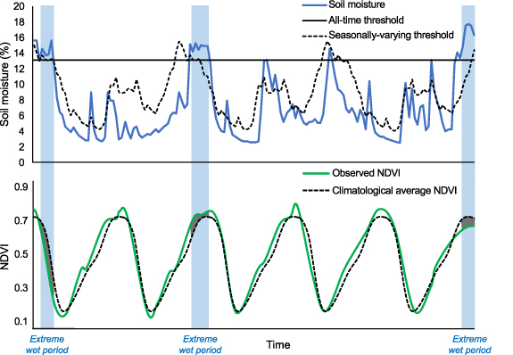
Figure 1. Simplified schematic diagram of extreme event identification and NDVI anomaly computation. Top subplot shows an example of a soil moisture time series (blue) along with its all-time threshold for wet events (solid black line, SMwet; see section 2.2) and seasonally-varying threshold for wet events at each 2 week period t (dashed black line, SMt ,wet). Extreme wet events, highlighted in light blue shading, occur when soil moisture observations surpass both thresholds SMwet and SMt ,wet. Bottom subplot shows observed NDVI (green) along with the NDVI climatology, or average annual cycle (dashed black line; see section 2.3). Differences between the two curves during extreme events (dark gray shading) represent NDVI anomalies used for further analysis.
Download figure:
Standard image High-resolution imageTo compute the all-time thresholds, a percentile-based cutoff for extreme dry events (SMdry) and one for extreme wet events (SMwet) were determined for each pixel using its full soil moisture time series. SMdry was equivalent to the soil moisture value at a chosen percentile p and SMwet was equivalent to that at 100 − p. In the main figures of this paper, p was set to 15 to ensure a sufficient sample size, although we tested the effects of several increasingly extreme values of p in a sensitivity analysis. Figure S1 (available online at stacks.iop.org/ERL/16/074014/mmedia) shows that our main results remain consistent across several choices of p.
To ensure that events identified as extreme based on SMdry and SMwet were not biased towards that pixel's driest and wettest seasons, we further imposed seasonally-varying thresholds to determine whether they were also extreme relative to their time of year. We computed dry-event and wet-event seasonally-varying thresholds for each 2 week period (t) of the year by assuming a Gaussian distribution of the interannual values of soil moisture. This approach differs slightly from that used to calculate the all-time thresholds because of the reduced number of observations available when only a certain time of year is considered. The seasonally-varying threshold for dry events (SMt ,dry) and that for wet events (SMt ,wet) were calculated as:
where  is the climatological average soil moisture at time t,
  is the z-score corresponding to percentile p (e.g.
  = 1.04 for p = 15), and
  is the standard deviation of observations yielding the climatology at timestep t.
To summarize, events identified as extreme using the all-time method were ultimately accepted only if they were also classified as such using the seasonally-varying method. That is, all soil moisture observations that fell below both SMdry and SMt ,dry were identified as extreme dry events and included in our analysis, and all that exceeded both SMwet and SMt ,wet were classified as extreme wet events (figure 1) and included. We note that regions for which soil moisture data were unavailable were necessarily excluded from the analysis.
We repeated the same extreme event classification procedure for both the radiation and temperature data. In order to ensure the events considered primarily reflected responses to hydrological rather than other climatic factors, any soil moisture extreme that co-occurred with a temperature or radiation extreme (22.9% of dry extremes and 19.0% of wet extremes) was removed from the analysis.
2.3. Identifying growing seasons from NDVI data
To identify growing seasons from the NDVI time series at each pixel, we first computed the NDVI climatology by averaging observations for each 2 week period across all years. This climatology represents the pixel's average annual cycle of NDVI. For each year, we identified the growing season as those values exceeding  , where
  is the peak and
  is the minimum of the average seasonal cycle, respectively. This approach is similar to previous efforts (White et al
1997, Vrieling et al
2013). Any soil moisture extreme that was identified but did not occur in a pixel's growing season was removed from the analysis.
is the minimum of the average seasonal cycle, respectively. This approach is similar to previous efforts (White et al
1997, Vrieling et al
2013). Any soil moisture extreme that was identified but did not occur in a pixel's growing season was removed from the analysis.
2.4. Computing average NDVI anomalies during extreme moisture events
For every pixel, we computed the average NDVI anomaly during extreme wet events (NDVIW) and the average NDVI anomaly during extreme dry events (NDVID) in the following way:

where  are the timesteps during which a total of
  extreme wet events occurred, j are the timesteps during which a total of
  extreme dry events occurred,
  and
and  are the NDVI observations at times i and j, and
  and
and  are the NDVI climatological averages corresponding to times i and j. Figure 1 shows how the extreme event identification procedure maps to NDVI anomalies.
NDVIW and NDVID were tested for statistical significance (student's t-test, p < 0.05) against all differences between observations and climatology over the entire record. Only significant values were included in the analysis.
2.5. Statistical comparison of distributions
We used the two-sample Kolmogorov–Smirnov test, or K–S test, to evaluate the equality of continuous climate and vegetation-related distributions (in particular, those tested as potential explanatory factors differentiating NDVIW from NDVID; see last paragraph of section 2.1). The test is used to assess whether two samples are statistically indistinguishable from one another (i.e. whether they were drawn from the same distribution). It returns the Kolmogorov–Smirnov statistic, which is the maximum distance between the empirical cumulative distribution functions of the two samples, as well as a p-value used for significance testing. No normality assumptions are required for its implementation. Theoretically, two dissimilar distributions will be characterized by a large Kolmogorov–Smirnov statistic, and two similar ones will have a small Kolmogorov–Smirnov statistic (figure S2). Here, results are included only for Kolmogorov–Smirnov statistics that were significant (p < 0.05).
3. Results
3.1. Regional-scale sensitivity to extreme wet and extreme dry events
Strong sensitivity hotspots exist for both wet and dry extremes, indicating regions for which vegetation greenness anomalies are strongly coupled to extreme hydrological events (figures 2(a) and (b)). High-magnitude sensitivities to both extreme wet events and extreme dry events appear in northeastern Australia and southern Africa, while many northern boreal regions are significantly sensitive only to the former and parts of India are only to the latter.
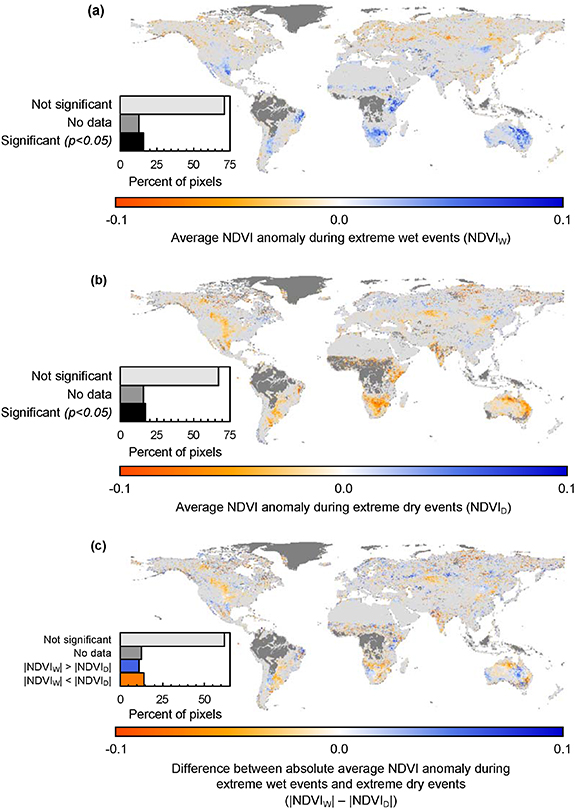
Figure 2. Maps of NDVIW, NDVID, and |NDVIW| − |NDVID|. (a) Average NDVI anomaly during extreme wet events (NDVIW). (b) Average NDVI anomaly during extreme dry events (NDVID). (c) Difference in magnitude between |NDVIW| and |NDVID|. Light gray pixels are not significant (student's t-test, p > 0.05). Dark gray pixels contain missing soil moisture data (for example, in tropical regions where dense vegetation can restrict the penetration of microwaves). Inset shows pixel frequencies. In panel (c), differences are computed only using significant values.
Download figure:
Standard image High-resolution imageFor 11.6% of the vegetated global land surface, average NDVI anomalies are larger in magnitude during extreme wet events than they are during extreme dry events (i.e. the absolute value of NDVIW exceeded that of NDVID), indicating a greater overall vegetation sensitivity to wetness than to dryness in those regions (figure 2(c)). This fraction is only slightly less than that for which NDVI is more sensitive to extreme dry events (14.4%; the remaining 74.0% is either not statistically significant or contains missing data (see inset of figure 2(c)). The near equivalence of these two fractions holds even when varying the soil moisture threshold used for identifying extreme events (figure S1) as well as when omitting agricultural regions from the analysis (figure S3), since their greenness responses may be skewed by irrigation use. Overall, this surprising result suggests that the spatial extents of the two types of vegetation sensitivities are comparable. That is, when sampling any specific location, it is almost as common for greenness to be more sensitive to wet extremes than to dry extremes.
Measures of average atmospheric moisture demand conditions, including mean PET, mean VPD, and the ratio of precipitation to PET (a common index of aridity), most strongly differentiate the class of pixels with high-magnitude NDVIW from those with high-magnitude NDVID (figure 3(a)). Specifically, pixels with the greatest sensitivity to wet events are characterized by lower aridity indices (figure 3(b); indicating PET far greater than the supply of water by precipitation), higher mean PET (suggestive of a larger moisture gradient, and thus a greater capacity for hydrologic exchange from the land to the atmosphere), greater VPD, higher radiation, and higher temperature than the most drought-sensitive pixels (figure S4). Notably, neither mean precipitation itself, nor precipitation variability, are strong differentiators between the two types of pixels (figure 3(c)), suggesting that moisture demand exerts a greater control than moisture availability over the spatial distribution of vegetation sensitivity to hydrological extremes. These climate-based distinctions also dominate differences in average land cover in their explanatory power. Mean LAI and mean NDVI were relatively similar between the two types of pixels, indicating representation from a broad range of vegetation covers, although pixels with lower temporal variability in NDVI tend to be more sensitive to wet extremes. Taken together, these results highlight the impacts of extreme hydrological events that oppose a region's dominant aridity regime, irrespective of its mean vegetation state, on greenness anomalies. Amid projections of enhanced wet extremes, they also draw attention to the future role of arid and semi-arid ecosystems in the global carbon cycle (Poulter et al 2014, Ahlström et al 2015).
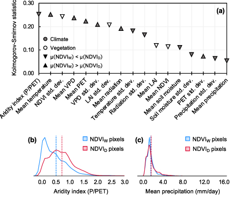
Figure 3. Differences in climate and vegetation between NDVIW pixels and NDVID pixels. A greater K–S statistic indicates more distinct distributions. (a) Maximum difference between cumulative distribution functions (Kolmogorov–Smirnov statistic) of NDVIW pixels and NDVID pixels for all variables. Upward-pointing triangles indicate that the mean of the NDVIW distribution for the given variable is greater than that of the NDVID distribution (e.g. NDVIW pixels have higher mean temperatures on average than NDVID pixels). Downward-pointing triangles indicate that the mean of the NDVIW distribution is less than that of the NDVID distribution (e.g. NDVIW pixels have lower aridity indices on average than NDVID pixels). Gray markers correspond to climate variables; white markers correspond to vegetation variables. All K–S statistic values shown are statistically significant (p <0.01). (b) Distributions of aridity index (largest K–S statistic) for the highest-magnitude NDVIW pixels and NDVID pixels. Dashed lines correspond to the mean of each distribution. (c) Distributions of mean precipitation (smallest K–S statistic) for the highest-magnitude NDVIW pixels and NDVID pixels. Dashed lines correspond to the mean of each distribution.
Download figure:
Standard image High-resolution image3.2. Sign of greenness change during extreme wet events
3.2.1. Spatial patterns
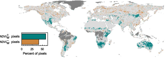
In 41.4% of pixels with a statistically significant response to extreme wetness, NDVI typically declines relative to its climatology during periods of extremely high moisture, while NDVI typically increases during these periods in 58.6% of pixels (figure 4). Note that for this analysis, we separated the subset of vegetated pixels for which NDVIW is positive (hereafter referred to as  ) from that for which it is negative (hereafter referred to as
  ) under extremely high moisture. There are regionally coherent patterns in the occurrence of
  and
and  pixels; regions like eastern Australia and southern Africa are dominated by
  pixels, while
  pixels account for large swaths of the northern high latitudes (figure 4). Most
  pixels are arid or semi-arid regions; they tend to be warmer and drier than
  pixels (figure S5), highlighting the ability of moisture-limited regions to translate even the most extreme additions of moisture over the 34 years record into increased greenness.
Figure 4. Map of NDVIW, colored by sign of response. Map of pixels with positive NDVIW ( ; shown in teal) and negative NDVIW (
 ; shown in brown). Inset shows the frequency of pixels in each class (calculated relative to the pixels for which NDVIW was significant at p < 0.05). Light gray pixels are not significant; dark gray pixels contain missing data.
Download figure:
Standard image High-resolution image
3.2.2. Event-scale controls on reduced greenness
While the analysis into spatial patterns largely explains the occurrence of positive NDVI anomalies during extreme wetness (i.e. they are predominantly linked to moisture-limited regions), the mechanisms contributing to reduced greenness during extreme wet conditions are more difficult to elucidate. To better understand such negative responses, we further focused on the timescale of individual extreme events. Though this approach inevitably includes significant uncertainties because our study uses observational data rather than controlled experiments, we identified two emergent patterns that may be interpreted as promising avenues for further research.
First, negative NDVI anomalies during extreme wet events tend to occur during growing seasons for which NDVI is already lower than average (figure S6(a)), suggesting that vegetation greenness was already depressed relative to the local climatology before the extreme event took place. This suggests that the occurrence of the extreme event, and the response by vegetation to it, may not be independent from the preceding climate conditions that caused the low-greenness observation. The magnitude of the NDVI anomaly is still greater—on average—during the wet extreme than before it, implying that this form of short-term memory influences the anomaly response but is not the sole cause.
Additionally, in some pixels, there is some evidence to support the hypothesis that a negative greenness response may be explained by excessive soil saturation, or waterlogging. Waterlogging can cause the soil to become so saturated that the plant cannot access enough oxygen to adequately respire (known as soil hypoxia). Soil hypoxia can decrease stomatal conductance and root hydraulic conductivity, among other negative impacts on plant growth and soil properties (Parent et al 2008). It is difficult to explicitly quantify the degree to which waterlogging occurs at a global scale, however, because it is not known how the soil moisture levels necessary to induce hypoxia vary across the globe. Furthermore, biases in soil moisture observations (Dorigo et al 2015) and global soil texture databases, which are likely a first order control on soil moisture levels required for saturation, would further complicate such an analysis.
As an indirect proxy for waterlogging, we considered different classes of extreme soil wetness, stratified based on the local soil moisture distribution. Across all pixels, wet extremes are distributed non-normally: that is, extremes occurring above that pixel's 95th percentile are more common than extremes occurring between its 90th and 95th percentile, which in turn are more common than those in the 85th-to-90th percentile class. Critically, however, it is more likely for events occurring at the highest soil moisture percentiles to yield decreased NDVI than to yield increased NDVI (table S1). It is therefore possible that a higher fraction of the wet extremes associated with reduced greenness may occur during waterlogged conditions. The possible role of waterlogging warrants further study as possible controls on the sign of the response by vegetation to extreme wetness.
4. Discussion
More attention to both types of extreme hydrological events—droughts as well as heavy precipitation—is needed to understand their impacts on vegetation now and in future decades. While which impact is dominant varies greatly across the land surface (figure 2(c)), many places exhibit significant sensitivities to both extreme wet and dry events (figures 2(a) and (b)). The carbon balance of such regions is therefore a function of multiple, dynamically evolving extreme event regimes. Coupled with the finding that the spatial extents of the two types of sensitivities are comparable, this contrasts with the significantly larger focus in the literature on dry, rather than wet, events (e.g. Farooq et al 2012, Schwalm et al 2017, Xu et al 2019).
The global distribution of  and
and  pixels demonstrated here aligns with prior work in grasslands suggesting that the response by terrestrial ecosystems to extreme rainfall events is highly nonlinear (e.g. Heisler-White et al
2008, Knapp et al
2008). However, our findings broaden the scope of such work in two key ways. First, our data-driven study indicates that bidirectional productivity responses (i.e. that productivity can either increase or decrease during extreme wetness) persist across far larger spatial and temporal scales than previously captured by field studies, and across biome types. Specifically, they persist across the scales relevant to informing and improving land surface models (which have been shown, for instance, to misrepresent the growth legacy effects of extreme wetness in many forests (Jiang et al
2019).
pixels demonstrated here aligns with prior work in grasslands suggesting that the response by terrestrial ecosystems to extreme rainfall events is highly nonlinear (e.g. Heisler-White et al
2008, Knapp et al
2008). However, our findings broaden the scope of such work in two key ways. First, our data-driven study indicates that bidirectional productivity responses (i.e. that productivity can either increase or decrease during extreme wetness) persist across far larger spatial and temporal scales than previously captured by field studies, and across biome types. Specifically, they persist across the scales relevant to informing and improving land surface models (which have been shown, for instance, to misrepresent the growth legacy effects of extreme wetness in many forests (Jiang et al
2019).
Second, we observed that controls on the sign of the greenness response under extreme wetness are also more complex than previously demonstrated under experimental conditions. While the observed sensitivity of arid regions is generally linked to average atmospheric moisture demand (figure 3), other factors—beyond mean climate conditions—may interact to impact the overall response by vegetation to extreme wetness in cases where greenness was ultimately reduced.
For instance, we took steps to isolate the impacts of extreme wet events on greenness (e.g. by only considering events that did not co-occur with radiation or temperature extremes; see section 2), but still found an inextricable effect of prior climate on both the magnitude and sensitivity of the vegetation response (figure S6). While previous work has focused on 'legacy effects' of extreme hydrological events on carbon fluxes (i.e. given an extreme event, how will vegetation respond in seasons to follow?) (e.g. Anderegg et al 2015, Jiang et al 2019, Gao et al 2020 at interannual timescales; or Schwalm et al 2017, Kolus et al 2019 at monthly timescales), we also found evidence of the inverse causality (a given prior vegetation anomaly exerts some control over its response to a later extreme wet event).
In particular, below-average carbon uptake—which may result from shifts in average temperature, cloud cover, or precipitation patterns diminishing photosynthetic rates—appears to affect the further depression of greenness during subsequent extreme wet conditions. A similar dynamic was identified by Randazzo et al (2020) in the context of linking synoptic meteorology to North American ecosystem carbon exchange at the site scale. It remains unclear, however, which prior climate conditions—and over what timescales—are most significant in affecting vegetation responses to later extreme wet events.
An additional limitation in understanding the tradeoffs between mechanisms controlling reduced greenness under extreme rainfall is the challenge of predicting where and when soil waterlogging, along with possible hypoxic or anoxic conditions, will occur. The occurrence of waterlogging and its consequences on plant functioning depend on both dynamic and static factors (including local and regional hydrology, soil texture, and slope position), and because of temporal gaps in soil moisture data and uncertainty in soil properties, it is often difficult to assess the prevalence of waterlogging directly at any given location.
Some evidence points to high-latitude regions as especially susceptible to over-saturated conditions. In particular, the fact that we observed a greater likelihood for NDVI-suppressing events in the northern high-latitudes (figure 4) is sensible given (a) the region's higher long-term average soil moisture relative to the consistently drier mid-latitudes (McColl et al 2017), (b) shallow groundwater tables in the region (Fan et al 2013), and (c) observations that in some of the most extreme northern ecosystems, melting snow, ice, and permafrost can further increase soil saturation (Turetsky et al 2007). Still, the properties of waterlogging (e.g. duration, time of year, climatological history) that most influence its effect on productivity, and how the likelihood of waterlogging varies through space and time across the land surface, remain unclear.
5. Conclusions
Using 34 years of satellite data, we found that regions more sensitive to extreme wet events than to extreme dry events are more prevalent than previously recognized. The greenness responses of those regions are not uniform; they are functions of multiple, often interacting, mechanisms (e.g. atmospheric moisture demand, average and preceding climate conditions, etc). Although regions where extreme wet events significantly affect vegetation greenness are widespread, the plant response to them remains poorly understood. In particular, the processes that control negative productivity responses to extreme wetness have not been studied in depth, and the relative roles and interactions of factors such as soil properties (Li et al 2019), the duration of soil hypoxia (Horchani et al 2008), or wind damage (Gardiner et al 2016) are not known. Similarly, while pre-event conditions influence the response to wet extremes (figure S6), the magnitude, pathways, and prevalence of that influence likely differ from region to region or event to event. Additionally, although events for which extreme soil moisture conditions coincide with extremes in temperature or radiation were excluded from this study, extreme wetness may also play an important role in regulating vegetation productivity during compound or co-occurring extremes (Zscheischler and Seneviratne 2017, Zscheischler et al 2018).
To parse the dynamics controlling the response to extreme wetness, future studies at higher spatiotemporal resolutions than the long-term global assessment here may benefit from recent advances in remote sensing of photosynthesis such as solar-induced fluorescence (Guanter et al 2014) or the near-infrared reflectance of vegetation (Badgley et al 2017), which more directly relate to carbon uptake than NDVI does. The increased study of extreme wet events is likely to improve forecasts of vegetation productivity, with further benefits for conservation, resource management, timber logging, and the quantification of ecosystem services.
Overall, the impacts of extreme hydrological events on carbon uptake will likely strengthen in a changing climate characterized by increasingly frequent and intense wet and dry periods. While it is possible that in some regions, the cumulative effects of droughts and extreme wet events will compensate on sufficiently long timescales (i.e. from year to year, reduced productivity during the former may be offset by increases during the latter), the prevalence of bidirectional responses to extreme wetness identified here, and the conditionality of its sign on a suite of interacting factors, complicate the likelihood of this outcome.
Data availability statement
The data that support the findings of this study are available upon reasonable request from the authors.
Acknowledgments
C A F, A M M, and A G K designed research. C A F processed and analyzed data. C A F, A M M, and A G K interpreted the results. C A F wrote the paper with support from A M M and A G K. All authors reviewed drafts of the manuscript. Feedback from three anonymous reviewers contributed to significant improvements in the manuscript's clarity.
Conflicts of interest
The authors declare that they have no competing interests.
Funding
CAF was funded by a Stanford Graduate Fellowship. A G K was funded by N O A A Grant NA17OAR4310127.