

Abstract
Lakes account for about 10% of the boreal landscape and are responsible for approximately 30% of biogenic methane emissions that have been found to increase under changing climate. However, the quantification of this climate-sensitive methane source is fraught with large uncertainty under warming climate conditions. Only a few studies have addressed the mechanism of climate impact on the increase of northern lake methane emissions. This study uses a large observational dataset of lake methane concentrations in Finland to constrain methane emissions with an extant process-based lake biogeochemical model. We found that the total current diffusive emission from Finnish lakes is 0.12 ± 0.03 Tg CH4 yr−1 and will increase by 26%–59% by the end of this century depending on different warming scenarios. We discover that while warming lake water and sediment temperature plays an important role, the climate impact on ice-on periods is a key indicator of future emissions. We conclude that these boreal lakes remain a significant methane source under the warming climate within this century.
Export citation and abstract BibTeX RIS
1. Introduction
Atmospheric methane (CH4) is the second major greenhouse gas after carbon dioxide. Although it only contributes to about 20% of the warming effect, its global warming potential is 28 times higher than carbon dioxide (Lashof et al 1990, Myhre et al 2013, IPCC 2014). Over the past two decades, surface freshwater including lakes, reservoirs, streams and rivers has been receiving an accumulating attention as important global methane sources (Bastviken et al 2011, Prairie et al 2013, Saunois et al 2016). However, studies have shown large uncertainties in the estimation of freshwater methane emissions (Kirschke et al 2013). A better estimation of the present and future lake methane emissions would largely benefit from critical improvement in watercourse mapping and methane flux measurements (Saarnio et al 2009; Kirschke et al 2013). Furthermore, previous studies mostly focused on quantitative estimation but hardly explored the mechanisms of how climate warming indeed affects lake methane emissions.
Finland has one of the densest inland water systems in the world with over 200 000 (Raatikainen and Kuusisto 1990) freshwater bodies covering an area greater than 33 000 km2 over the whole country. Nearly all the lakes are in the boreal region. Ranta10 (Finnish Environment Institute 2016) is a topologically corrected spatial dataset. It contains geographical coordinate and area information of 214 995 lakes, covering 37 595 km2 of the land surface. It is higher in spatial resolution than the more commonly used Global Lakes and Wetlands Database (GLWD) which only comprises 2202 lakes and reservoirs covering around 20 194 km2 in Finland. The Ranta10 database offers a unique opportunity for modeling exercises since the smaller lakes are found to have higher methane fluxes per unit area (Juutinen et al 2009, Holgerson et al 2016, Sasaki et al 2016) and are more sensitive to climate change (Sanches et al 2019). Additionally,( Juutinen et al (2009) have provided the measured water temperature, nutrients and methane concentrations for the studies 207 Finnish lakes.
By using these datasets, we can not only evaluate methane emissions from the boreal lakes in Finland under climate change through modeling but also further explore the driving factors of emissions from a mechanistic perspective, which shall help future prediction of the emissions under climate change. Also, we extrapolate our model to the whole Arctic freshwater system for both historical and future periods.
2. Materials and methods
2.1. Model configuration
The Arctic Lake Biogeochemistry Model (ALBM) is a one-dimensional process-based lake biogeochemical model designed for predicting both thermal and carbon dynamics of aquatic ecosystems. It mainly consists of several modules including those for the radiative transfer, the water/sediment thermal circulation, the water/sediment biogeochemistry, and the gas diffusive and ebullition transportation. Although this model was originally developed for Arctic lakes (Tan et al 2015a), it can achieve comparable or even better performance than those widely used one-dimensional lake models in representing the physical and biogeochemical processes of other northern lakes (Guseva et al 2020). Detailed information about ALBM can be found in Tan et al (2015a, 2017, 2018). We introduce the key governing equations of methane processes in ALBM below.
Methane production rate P (μmol m−3 s−1) in sediments is calculated from labile carbon content and temperature:
where  is the fraction of carbon decomposed per second (s−1),
  is the labile carbon content (μmol m−3), PQ10 is the factor by which the production rate increases with a 10 °C rise in temperature, and Tpr is a reference temperature (°C). Methane can be oxidized after released into the water and the oxidation rate Voxid (μmol m−3 s−1) is described by
where  is the maximum oxidation potential (μmol m−3 s−1), OQ10 is the factor by which the oxidation potential increases with a 10 °C rise in temperature, Tor is a reference temperature (°C),
  and
and  and gas concentrations (μmol m−3), and
  and
and  are the Michaelis-Menten constants (μmol m−3). Together, the modeled methane concentration in water columns is calculated by
where  is the diffusivity of methane (m2 s−1), and
  is the gas exchange between bubbles and the ambient water (μmol m−3 s−1). Finally, methane within water is transported to the atmosphere. The diffusive transfer velocity k (m s−1) is defined as
where U is the wind speed at 2 m (m s−1), β is buoyant flux (β < 0 if losing heat and vice versa), zAML is the depth of the actively mixing layer (m), and Scm is the Schmidt number of methane. Since we lacked ebullition flux observations and therefore, we were unable to validate the modeled ebullition emissions, we only quantified diffusive emissions in this study.
The numerical experiment consists of three steps: (1) the model calibration using observations of diffusive emissions during 1998–1999 from 39 individual lakes; (2) regional simulations of 1990–1999 by applying ALBM to the Ranta10 data product; (3) regional simulations of 2010–2019 and 2090–2099 under the representative concentration pathway (RCP) scenarios of RCP4.5 and RCP8.5. For all the simulations, a spin-up period of two years was run.
2.2. Data
Model forcing data include air temperature, surface pressure, 10 m wind, relative humidity, precipitation, snowfall, downward short-wave radiation and downward long-wave radiation. The historical simulation was driven by the climate data retrieved from the European Center for Medium-Range Weather Forecasts (ECMWF) Interim re-analysis (ERA-Interim, Dee et al 2011) with a resolution of 0.75° × 0.75°, and organized into daily datasets. For future climate scenarios, we used a down-scaled bias-corrected dataset of the Intersectoral Impact Model Intercomparison Project (ISIMIP) output from HadGEM2-ES (Frieler et al 2017) that is set on a 0.5° × 0.5° global grid and is divided into daily time steps. This climate dataset is bias-corrected based on ERA-Interim, which guarantees the consistency of historical and future simulation results.
Lakes with an area smaller than 200 m2 were omitted in our simulations due to the large uncertainties in the mapping of these lakes, leaving 176 876 lakes covering 36 690 km2. In general, the region north of 67 °N has the highest lake density but relatively sparse observations of thermal or carbon dynamics (figures 1(a) and 1(b)). Over 90% of the lakes are smaller than 0.1 km2 (figure 1(c)), which are not included in the GLWD-3 database. Depth information was lacking for over 90% of the lakes even by combining the Ranta10 and the GLWD-3 database. As such, we applied a statistical approach to construct the full lake depth dataset. We first grouped the lakes into 10 bins bounded by areas of 0, 0.01, 0.05, 0.1, 0.5, 1, 2, 3, 4, 5, 10, 100, 1500 km2, respectively. We then generated a histogram of depths in each group. We randomly assigned the depths following the fitted probability distribution in each group. By following this approach, we aimed to construct lakes profiles that match the diversity of the real lake system in Finland. In terms of lake bathymetry, we assume a linear decrease of the cross-section area with increasing depth.
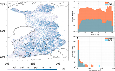
Figure 1. Map of Finland with lakes color coded by surface area (a). Triangles indicate the lakes used for calibration. Distribution of lake latitudes in Ranta10 (orange) and GLWD (blue, b). The same as (b) but for lake surface areas (c). Note that the y-axis starts from 1 so some of the large lakes do not show up.
Download figure:
Standard image High-resolution imageWater temperature, nutrient and methane concentrations were measured at four levels of depth four times (before and after ice melt, late summer and autumn circulation) either in the 1998 or 1999. The diffusive methane fluxes were calculated following equation (4) (see also Juutinen et al 2009). For the simulation purpose, several assumptions and approximations were made on for carbon and phosphorous input that is required by the model, including (1) dissolved organic carbon (DOC) concentration is equal to total organic carbon (Mattsson et al 2005, Kortelainen et al 2006, Mopper et al 2006); (2) dissolved inorganic carbon (DIC) concentration is calculated from pH and alkalinity; (3) soluble reactive phosphorus (SRP) concentration is equal to PO4 and (4) particular organic carbon (POC) concentration is approximately 1/5.1 of DOC concentration (Rachold et al 2014). We produced an input map of DOC, DIC, PO4 and SRP at 1° × 1° with observations averaged at each grid and filled with nearest-neighbor interpolation (figure S1 (stacks.iop.org/ERL/15/064008/mmedia)).
2.3. Model calibration
Since the lake shape has large impacts on the thermal dynamics (Mazumder and Taylor 1994, Woolway et al 2016, Woolway and Merchant 2017) and carbon dynamics (Schilder et al 2013, Pighini et al 2018), we decided to conduct calibration and thus simulations by lake groups. The simulated lakes were firstly divided by the surface area into six groups bounded by 0, 0.05, 0.1, 0.2, 1, 10, 1500 km2, respectively and then by the shape factor, defined by  , into two groups bounded by 0, 0.1 and 10, respectively. Thirty-nine lakes that represent various depths and shape factors were used for calibration.
We calibrated the parameters related to water temperature (Ks, Cps, Pi, Rous, Roun, Feta, Wstr and Ktscale) and methane diffusive emission (OQ10, QCH4, KCH4, PQ10 n, Rcn and Rca as in equations (1) ∼ (4)). The detailed descriptions and corresponding ranges of the parameters are listed in table S1. Since the sensitive parameters of the water temperature and the methane diffusive emission simulations were different, the calibration was conducted separately. We first applied a Monte Carlo calibration method for water temperature calibration using 6000 sets of parameters for each lake. For the methane emissions, a 'history matching' method (Mcneall et al 2013, Williamson et al 2013, 2015, 2016) was adopted for higher accuracy and efficiency. This method requires less computation time than a full Monte Carlo simulation (Williamson et al 2013) and has been shown to largely reduce simulation biases (Salter et al 2019). It was carried out in the following steps: (1) use the Sobol sequence sampling method (Sobol' 1967) to generate a perturbed parameter ensemble (PPE) by sampling from the parameter space; (2) run simulations for all perturbed parameter (PP) sets; (3) rule out regions of the parameter space based on the outputs where a predefined metric exceeds the threshold; (4) repeat step 1–3 until a certain number of iterations or the desired outcome is achieved. In our study, 1200 PP sets were generated for each round and the metric used was the root-mean-square error (RMSE). Parameter spaces resulting in RMSEs over the 50% of the observations at each site were ruled out at each round, until 3 rounds were finished.
2.4. Sensitivity and uncertainty analysis
For parametric sensitivity analysis, running the model for the whole region over a 10-year time period takes about five days, and thus it would be rather time-consuming to run full PPE simulations. Instead, we run short PPE simulations for a single year from 1998 to 1999 with 20 PP sets sampled from the remaining parameter space after history matching. It has been proved that the results from short simulations match well to the longer-term simulations (Yun et al 2016), especially when methane emission response to air temperature is a relatively well-defined process (Sanches et al 2019) and thus can be captured within a one-year range.
3. Results and discussion
3.1. Model performance
The model overall showed good performances on reproducing both water temperature and methane emissions (table 1) with an average RMSE of 1.59 °C for full-profile water temperature simulations and a correlation coefficient (r) of 0.69 for methane emissions. There was a lake with an estimated methane flux over 200 mmol m−2 yr−1 while the corresponding modeled value was only one-third of the observed value. This underestimation was possibly due to the missing of DOC concentration measurement at this lake. Since it is a very humic shallow lake (color >90 Pt mg l−1, mean depth <3 m, see Juutinen et al 2009), taking the average value of other lakes in the same grid likely results in a much lower DOC concentration. The metrics without considering this lake are also listed in table 1.
Table 1. RMSE and r values of water temperature and methane flux simulations. Values in brackets are calculated without considering the very humic shallow lake.
| Annual mean full-profile water temperature | Annual mean methane flux | |
|---|---|---|
| RMSE | 1.59 °C | 32.91 (24.07) mmol m−2yr−1 |
| R | 0.94, p < 0.0001 | 0.69 (0.76), p < 0.0001 |
Note that the uncertainty range can be wider using the history matching approach than using the Bayesian method, which is expected because the former focuses on confining the output whereas the latter on confining the input, i.e. the parameters themselves. Therefore, the PPE by the latter would be more representative of the parameter distributions and thus results in smaller uncertainties.
3.2. Annual methane emission estimation
Simulations indicated that the methane emissions from Finnish lakes were 0.12 ± 0.03 Tg CH4 yr−1 in the 1990 s. There was only a 4% and 6% increase during the period 1990 ∼ 2019 under RCP4.5 and RCP8.5, respectively (figure 2) when less than 2 °C of warming has occurred. Walter et al (2007) estimated that the current total diffusion from all lakes north of 45 °N is 1.12 ± 0.22 Tg CH4 yr−1. If assuming the same total lake area over the Arctic and the same lake size distribution as the Finnish lakes (Text S1), we estimated the emission to be 3.65 ± 1.06 Tg CH4 yr−1. The difference can be due to: (1) Walter et al (2007) simply used a constant flux calculated from several glacial lakes and thermokarst lakes for all other lakes, which may underrepresent the variation; (2) Based on several Siberian thaw lakes, an ice-free period of 120 d was assumed in the calculation for all lakes, leading to underestimation in warmer regions, for example, the mean ice-off periods in Finland is about 170 d.
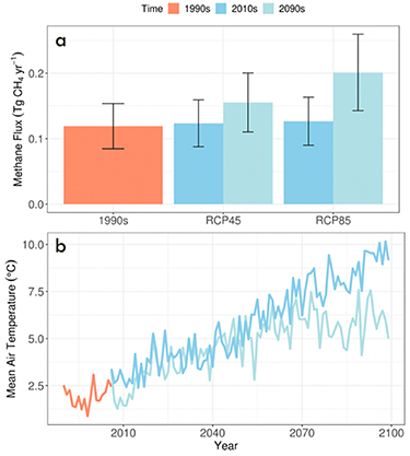
Figure 2. Simulated diffusive methane emissions (a) and mean annual air temperature (b).
Download figure:
Standard image High-resolution imageWe estimate that the Finnish lake diffusive methane emission will increase by 25.8% from 0.12 ± 0.04 to 0.16 ± 0.05 Tg CH4 yr−1 under the RCP4.5 scenario while it will increase by about 58.9% from 0.13 ± 0.04 to 0.20 ± 0.06 Tg CH4 yr−1 under the RCP8.5. The magnitude of the growth is relatively small compared to Tan et al (2015a) and Tan and Zhuang (2015b)) who predicted an 80% increase in Northern Europe even under the RCP2.6 scenario. It is likely because we did not model ebullition emission. It has been found that future warming may have much larger effects on ebullition even altering diffusive-emission dominant lakes to ebullition-dominant ones (Aben et al 2017). Therefore, the amount of extra increase is likely due to the enhanced ebullition processes.
Based on the analysis of 297 lakes worldwide, Sanches et al (2019) found that considering only diffusive emissions would cause an average underestimation of 277%. By taking into account the ebullition emissions, the current annual methane emission for all northern lakes would be 13.76 ± 3.99 Tg CH4 yr−1, in the lower range of the previous estimation, 24.2 ± 10.5 Tg CH4 yr−1 by Walter et al (2007) and about the same as the 16.5 ± 9.2 Tg CH4 yr−1 by Wik et al (2016). Furthermore, Aben et al (2017) predicted that ebullition would increase faster than diffusive emissions, by 51% with 4 °C warming. Similarly, Thornton et al (2015) predicted an increase of around 56% from the present to the 2040–2079 period using observations from three subarctic lakes in Sweden. If, based on the warming magnitude, we estimate a 50% and 100% growth of ebullition emissions under the RCP4.5 and RCP8.5, respectively, this will result in a total methane emission of 20.02 ± 5.8 Tg CH4 yr−1 and 27.97 ± 8.11 Tg CH4 yr−1, respectively from the whole Arctic lakes. This projection is slightly lower than the previously modelled 32.7 ± 5.2 Tg CH4 yr−1 from lakes north of 60 °N using the GLWD map by Tan et al (2015b). Their potential overestimation can result from: (1) They calibrated the model using only five lakes, four of which are thermokarst lakes that are found to have higher ebullition to diffusive emission ratio than other types of lakes (Wik et al 2016). According to their observation, this ratio can be over 30 which is much higher than we assumed; (2) They also assigned a shallow depth of 3 m to all lakes missing depth information, leading to even more overestimation of the ebullition emission (Joyce and Jewell 2003, Bastviken et al 2004, Del Sontro et al 2016).
3.3. Spatial variation in methane emissions and response to warming
Methane emissions are generally highest in regions dense with small lakes (figures 1(a) and 3), a pattern which was also found in previous studies (Bastviken et al 2004, Saarnio et al 2009, Del Sontro et al 2016, Wik et al 2016). This finding can be explained with two mechanisms. First, methane can be oxidized along diffusive transportation, and thus deeper lakes usually mean more loss by oxidation. Second, it was found that smaller lakes are more likely to have abundant organic substrates in their sediments, and thus they are potentially more productive for methane.

Figure 3. Annual mean methane fluxes weighed by lake surface areas during the 2010s under the RCP4.5 (a), the 2090s under the RCP4.5 (b), the 2010s under the RCP8.5 (c) and the 2090s under the RCP8.5 (d).
Download figure:
Standard image High-resolution imageInterestingly, the southern and the northern part of Finland show different trends. By the same 4 °C of air temperature warming (figure S2), the south experiences a much more severe increase in emissions than the north (figure S3). Here we define the south and north be distinguished by latitude 67.5 °N, which north and south mean annual air temperature is above or below 0 °C in the 2010s, respectively. Therefore, the absolute increase in air temperature is not a complete proxy for emission. Instead, we found that the length of ice-free days plays a key role. By the end of the century, the mean ice-free days in the north are extended by 10.8% and 23.5% under RCP4.5 and RCP8.5, respectively while they are extended by 13.2% and 34.1%, respectively in the south (table S3). Methane fluxes can be blocked by ice cover and then oxidized in the water column during ice-on seasons. Therefore, a large amount of methane trapped by ice cover currently could be emitted into the atmosphere in the future. Generally, ice covers of lakes in the north are thicker and thus would take more energy input to melt before methane can be released in winter.
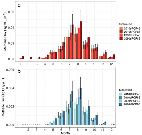
The influence of ice-on days is further verified by the seasonality of emission (figure 4). From May to November, the warming climate affects emission in a similar pattern in both regions. However, the difference is shown in the south from December to April when we hardly see any emissions in the 2010s, but we expect much higher emissions in the future for the period due to warming. Such a shift may not be initiated in the north within this century and thus, the increase of emission in the north is much less severe. Wik et al (2014, 2016) also indicated that the ice-free days could potentially be the primary proxy for emission based on the observation of three lakes. Here, we confirm the finding with all the lakes in Finland and further verify it from a seasonality perspective. They predicted a 30% increase in total emission from northern lakes within the century by assuming a 20-day increase of ice-free days for all lakes. However, we emphasize that differentiating assumptions on ice-free day increase among regions is necessary for better precision in the estimation of regional budgets and future projections. Additionally, our simulated increase of ice-free days under RCP8.5 is two to three times higher than their assumption, indicating an underestimation in the previous study.
Figure 4. Monthly methane emissions from lakes south (a) of and north (b) of 67.5 °N, respectively. Note different scales on y-axis.
Download figure:
Standard image High-resolution image
3.4. Uncertainty quantification
Our model simulations did not consider the impacts of DOC dynamics on lake methane emissions. Boreal lakes, in addition to the climate change, have experienced moderate to severe browning over the last decades, probably due to the increased import of DOC from soils (Roulet et al 2006, Monteith et al 2007, Haaland et al 2010, Larsen et al 2011, Seekell et al 2015, Isidorova et al 2016). If DOC concentrations increase at the current rate, they can be doubled by the end of this century (de Wit et al 2016). It is found that methane diffusive methane emission is positively related to DOC concentrations (Sanches et al 2019). However, the relationship can involve several processes. More nutrients will be available for microbes and primary producers. However, the resulting increases in turbidity will weaken photosynthesis and thus oxygen production which limits methane oxidation. The model will need to be improved to predict the effect of lake browning. So far, no study has included this effect when estimating future emissions.
We assumed a constant landscape in our simulations that no lake expansion or drainage was considered until 2100. This is because boreal lakes in Finland are not formed over permafrost and thus not affected by the active response of thawing and groundwater penetration processes in responding to climate as thermokarst lakes (van Huissteden et al 2011, Katey et al 2018). Wik et al (2016) predicted that with a 20-day increase of ice periods, even the total lake area decreases by 30%, the total methane emission can still grow by 20% which is 10% less than assuming constant lake area. Therefore, we will still expect the boreal lake methane emissions will be affected by considering the lake area changes. Incorporating lake areal dynamics into future quantification is necessary.
4. Conclusions
Lakes are an important component of the arctic and subarctic landscape. Our process-based lake biogeochemistry model simulation reveals that diffusive methane emissions from boreal lakes in Finland amount to 0.12 ± 0.03 Tg CH4 yr−1 during the 1990s and will increase by 25.8%–58.9% by the end of the 21st century depending on the warming scenario. There are two main driving factors. We find that higher air temperature will lead to higher lake water temperature and thus more active methanogenesis. Warming also results in shorter ice-on periods, leading to longer emission days. The ice-free days are a more dominant factor than the lake temperature change impacts. If extrapolating the ratio of diffusion to ebullition emissions to the region, we estimated the annual regional lake emissions are 13.76 ± 3.99 Tg CH4 yr−1 at the present and 20.02 ± 5.8–27.97 ± 8.11 Tg CH4 yr−1 during 2090–2099 from all lakes north of 45 N. Apart from climate forcing, lake trophic state, which we lack observation and future projection of, can also affect lake carbon and methane dynamics significantly. A more accurate estimation of lake methane emission requires both an increase in field measurement and improvement of the model structure. Furthermore, incorporating landscape evolution including lake drainage and expansion will refine our quantification of lake methane emissions in the future.
Acknowledgments and Data
This study is supported through a projected funded to Q Z by NASA (NNX17AK20G) and a project from the United States Geological Survey (G17AC00276). Z T is supported by the U.S. DOE's Earth System Modeling program through the Energy Exascale Earth System Model (E3SM) project. Narasinha Shurpali acknowledges support from the CAPTURE project (Project No. 296887, Academy of Finland). The supercomputing is provided by the Rosen Center for Advanced Computing at Purdue University. The Ranta10 dataset is available at https://www.syke.fi/en-US/Open_information/Spatial_datasets/Downloada ble_spatial_dataset#R. The model input and output data that support the findings of this study are openly available at https://purr.purdue.edu/publications/3391/1.