

Abstract
Multi-hazard assessment is needed to understand compound risk. Yet, modelling of multiple climate hazards has been limitedly applied at the global scale to date. Here we provide a first comprehensive assessment of global population exposure to hydro-meteorological extremes—floods, drought and heatwaves—under different temperature increase targets. This study shows how limiting temperature increase to 1.5 and 2 °C, as for the goals of the Paris Agreement, could substantially decrease the share of global population exposed compared to a 3 °C scenario. In a 2 °C world, population exposure would drop by more than 50%, in Africa, Asia and the Americas, and by about 40% in Europe and Oceania. A 1.5 °C stabilization would further reduce exposure of about an additional 10% to 30% across the globe. As the Parties of the Paris Agreement are expected to communicate new or updated nationally determined contributions by 2020, our results powerfully indicate the benefits of ratcheting up both mitigation and adaptation ambition.
Export citation and abstract BibTeX RIS

Original content from this work may be used under the terms of the Creative Commons Attribution 4.0 license. Any further distribution of this work must maintain attribution to the author(s) and the title of the work, journal citation and DOI.
1. Introduction
The Parties of the Paris agreement committed to keep global temperature increase well below 2 °C compared to pre-industrial levels (UNFCCC 2015, 2016), and to strive for limiting it to 1.5 °C. The IPCC Special Report on the impacts of global warming of 1.5 °C (SR15) evidenced how this temperature goal would decrease risks to natural and human systems and ease adaptation responses to climate-related extremes (IPCC 2018). Yet, countries' mitigation actions, as pledged in their nationally determined contributions (NDCs), currently fall short of the ambition. The aggregate effect of current NDCs could lead to a warming of between 2.6 and 3.1 °C by the end of the century, if no deep transformations of the energy, transport, industry, and land-use sectors are undertaken (Rogelj et al 2016, IPCC 2018, Vrontisi et al 2018). As Parties are requested to communicate new or updated NDCs by 2020, there is an urgent need to ratchet up ambitions to avoid the most dangerous consequences of climate change.
The SR15 explored the implications of crossing temperature thresholds, and assessed the impact of recent climate change (1 °C of warming compared to pre-industrial levels) and the likely impact of additional warming of 0.5 and 1 °C (Hoegh-Guldberg et al 2019, 2018). At 1.5 and 2 °C global warming, heatwaves are projected to become more frequent and longer. Significant changes in temperature and precipitation extremes were already observed comparing the period 1991–2010 with respect to 1960–1979 (about 0.5 °C of warming compared to pre-industrial levels). The risks of drought, dryness and precipitation deficits are likely to increase in some regions, and the areas affected by river floods are projected to increase (Hoegh-Guldberg et al 2018). Despite recognizing that some regions will be affected by collocated or concomitant changes in several hazard types (Hoegh-Guldberg et al 2018), the SR15 considers hazards in isolation. Quantitative modelling of multiple climate hazards has seen to date only a limited number of applications (Forzieri et al 2016, Harrington and Otto 2018, Arnell et al 2019, Aghakouchak et al 2020, Batibeniz et al 2020), especially at the global scale. A key challenge is the identification of consistent approaches that use unbiased indicators to incorporate all hazards with their appropriate weight (Aghakouchak et al 2020). In addition, non-linearities due to the coexistence of multiple hazards within the same disaster (e.g. heatwaves and drought, or flooding in combination with extreme precipitation, wind and hail storm) are rarely considered in the biophysical impact assessment (Kappes et al 2012, Gallina et al 2016). Yet, recent coordinated efforts have shown trends towards integrated multi risk assessment through the use of a common set of climate forcing and underlying assumptions, as well as with the estimation of secondary economic effects through a common macroeconomic modelling framework (European Commission 2020).
Multi-hazard assessment is needed to understand compound risk (IPCC IPCC, 2012aa, Pescaroli and Alexander 2018), and thus improve projections of potential high-impact events (Gallina et al 2016). Here, we focus on three hydro-meteorological extremes, namely floods, droughts, and heatwaves, and assess how their combination with evolving socioeconomic dynamics—in terms of exposed population—amplifies their overall impact under future climate scenarios. In particular, making use of an ensemble of climate projections, we investigate to what extent limiting warming to 1.5 and 2 °C, as for the Paris Targets, could decrease the share of global population exposed to hydro-meteorological extremes, compared to a 3 °C world, which is consistent with the current NDCs (Raftery et al 2017).
Several studies have used the climate projections derived from the Coupled Model Intercomparison Project phase 5 (CMIP5) (Taylor et al 2012) to assess the changing frequency and magnitude of the extreme hydro-meteorological events in specific periods of the coming decades (Seneviratne et al 2012, Schellnhuber et al 2014, Mora et al 2018). Other studies (Sedláček and Knutti 2014, Byers et al 2018, Madakumbura et al 2019, Arnell et al 2019), investigated the impact of different global warming levels (GWLs) on several hazards (UNFCCC 2016). Our analysis rigorously assesses the various aspects of the combination of the three hazards, as for time, frequency, magnitude, and spatial distribution. Specifically, we rely on a set of high resolution projected indicators for heatwave (Dosio et al 2018), drought conditions (Naumann et al 2018), and river flood (Alfieri et al 2017) developed within the High-End cLimate Impacts and eXtremes (HELIX)6 project (Betts et al 2018), designed to produce information about climate change adaptation and mitigation policy strategies. The multi-hazard analysis is then combined with projections in population growth from compatible shared socio-economic pathways (SSP) (Riahi et al 2017). The study provides a first comprehensive assessment of the global population exposure to hydro-meteorological extremes under and beyond the Paris Targets, and thus makes a strong case for more ambitious mitigation and adaptation policies in the context of the 2020 update of NDCs.
2. Results
We analyse the evolution of the magnitude and frequency of the combined hazards—droughts, heatwaves, and floods- for the 1.5, 2 and 3 °C scenarios (figures 1(a)–(d)). Results are aggregated and visualized in macro geographical regions (Iturbide et al 2020, figure S1 (available online at stacks.iop.org/ERL/15/104037/mmedia)). The first and third panels in figure 1 show the overall multi-hazard magnitude for the modelled baseline (1981–2010, see table S1) and the 2 °C GWL, respectively (figures 1(a), (c)). In the baseline, droughts and floods jointly represent almost the total amount of the multi-hazard in all regions (figure 1(a)). Compared to droughts, floods play a major role in terms of contribution to the overall magnitude, but, at least in the developed world, a lesser role in frequency: this is likely due to the level of flood protection infrastructure in place in the most developed and in the fastest developing countries (Alfieri et al 2017). While the flood and drought indexes are quantified in comparison to long-term average conditions, the heatwave magnitude index is calculated as a change from historical observations (see Methods) (Dosio et al 2018). This explains the relatively minor representation of heatwaves in the baseline (figure 1(a)) even if strong heatwaves have heavily struck many regions of the world during the reference period (Aghakouchak et al 2020).
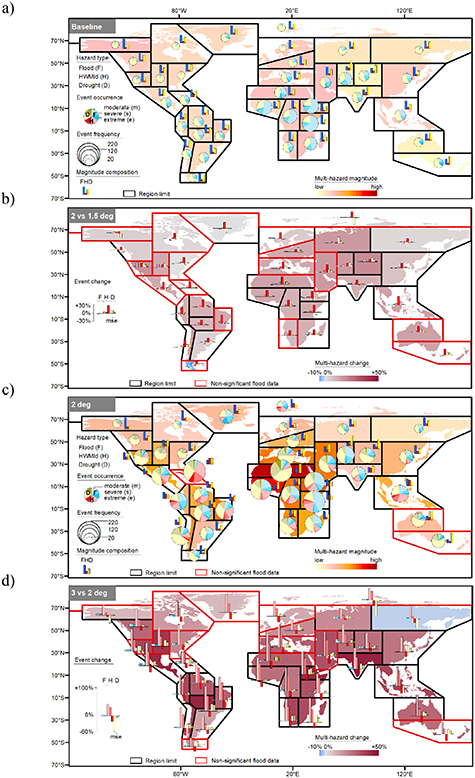
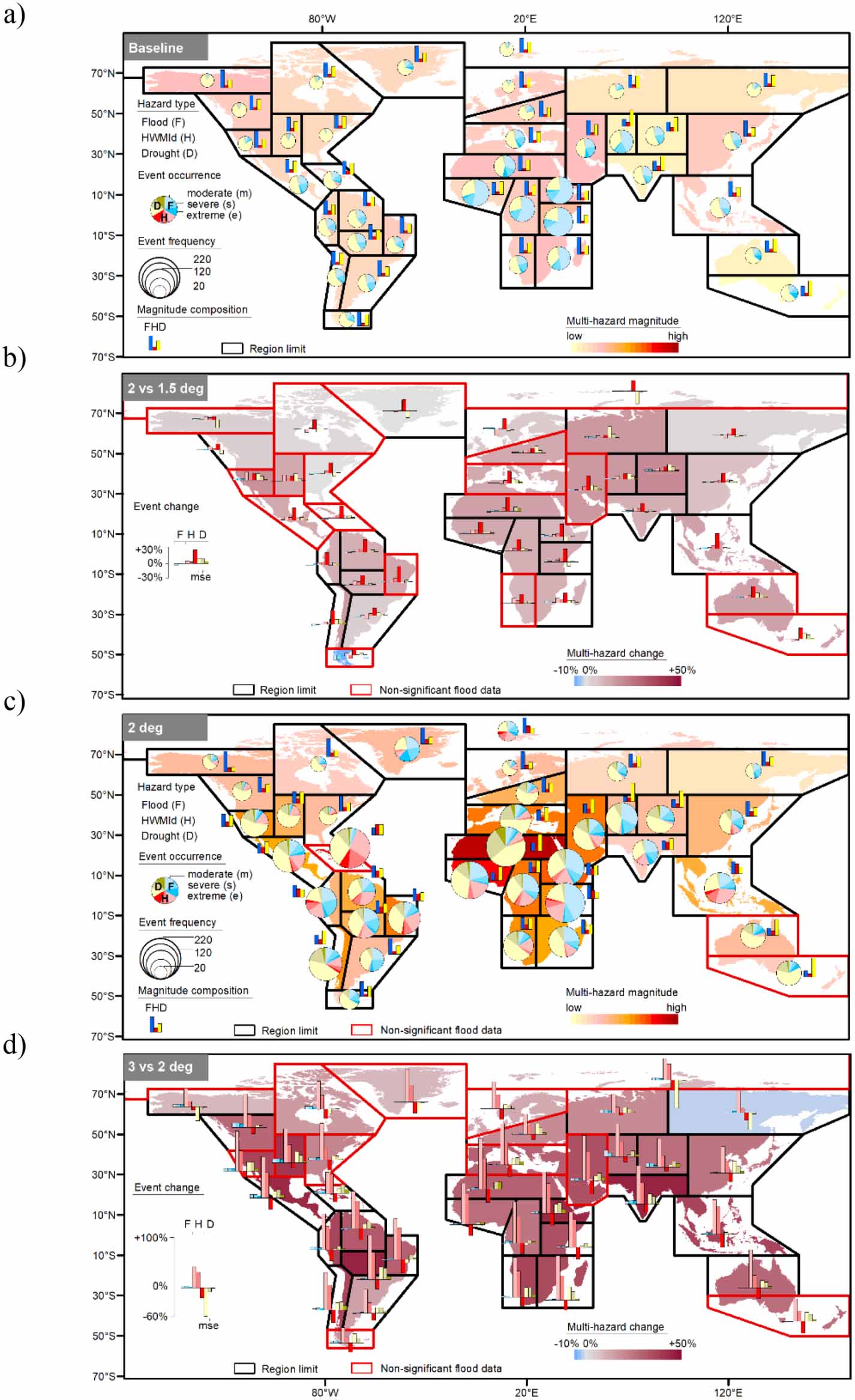
Figure 1. Multi-hazard evolution in a 1.5, 2 and 3 degree warmer world. Modelled Baseline and 2 degree panels (a) and (c), respectively) report the overall multi-hazard magnitude (normalized scale 0–300) averaged by region. 1.5 vs 2 degree and 3 vs 2 degree panels (b) and (d) are expressed in percent change. Bar charts in the baseline and 2 degree panels represent the relative magnitude of the three hazards (F = Flood, H = Heatwave, D = Drought). Pie-charts in the baseline and 2 degrees panels represent the frequency (pie size) of the events stratified in magnitude classes (moderate, severe, extreme). Bar charts for 1.5 and 3 degrees represent the percent change of the three hazards (F = Flood, H = Heatwave, D = Drought) divided in their magnitude classes (moderate, severe, extreme). Red areas indicate statistically non-significant changes in the flood data (changes in the other two hazards are statistically significant in all the scenarios).
Download figure:
Standard image High-resolution imageIn a 2 °C world, with respect to baseline, both the magnitude and frequency of the combined hazards significantly increase in the most temperate areas of the Americas (North +48%, Central +122%, South +67% in magnitude), Europe (+36%) and Mediterranean (+86%), Africa (+93%), Central (+82%) and South-Eastern (+56%) Asia due to a large increase in heatwaves and droughts (figure 1). Changes in the magnitude and frequency of heatwaves and droughts are statistically significant in all scenarios for all regions. This is not the case for floods, as changes are generally not noticeable in dry areas, and the high level of flood protection infrastructures in developing countries does not allow for detecting significant increases in flood magnitude for different GWL (figures 1(b) and (d)). In addition, some literature suggested a weak streamflow response to precipitation increase in a warming world. Streamflow response, in fact, is determined by the catchment characteristics further to the precipitation changes (Wasko and Sharma 2017, Sharma et al 2018). Nevertheless, changes in flood magnitude and frequency, when comparing a 2 °C world with the reference scenario, are significant throughout the globe, except for the Caribbean and Oceania (figure 1(c)).
Limiting the temperature increase to 1.5 ºC, would result in more than a 10% reduction of the multi-hazard magnitude globally when compared to 2 °C (figure 1(b)), and in particular in Africa (−11%), Mediterranean (−12%), Central Asia (−16%), the Tibetan Plateau (−20%), Central America (−14%), and in Central (−13%) and South-Western (−19%) North America. Large part of the decrease in the multi-hazard combination is due to less frequent and intense heatwaves in the 1.5 °C scenario compared to the 2 °C (−47% in magnitude globally). The decrease in magnitude and frequency of droughts is less relevant and concentrated in Central Europe (−26%), Mediterranean countries (−19%), and Central Asia (−22%). A decrease in the magnitude and frequency of flood events, instead, is only evident in East Africa (North −8%, Central −5%, South −6%) and Central Asia (−5%). In a 3 °C scenario, the multi-hazard magnitude increases almost all over the globe (+30%), and in particular in areas that are already significantly hit at lower levels of warming. The most considerable changes would affect Africa (+37%), Central America (+48%) and the Caribbean (+43%), and Central (+30%) and South-Eastern (+40%) Asia, while minor changes are expected at the high and very high latitudes (figure 1(d)). Overall, heatwaves are the main drivers of change (global magnitude increase: +100% with 1.5 °C, +200% with 2 °C, and +498% with 3 °C compared to the baseline scenario), followed by droughts (+48%, +65%, and 107%, respectively), which are increasing consistently for all the GWL, and floods (+33%, +36%, and +48%, respectively) (figures 1(a)–(d)).
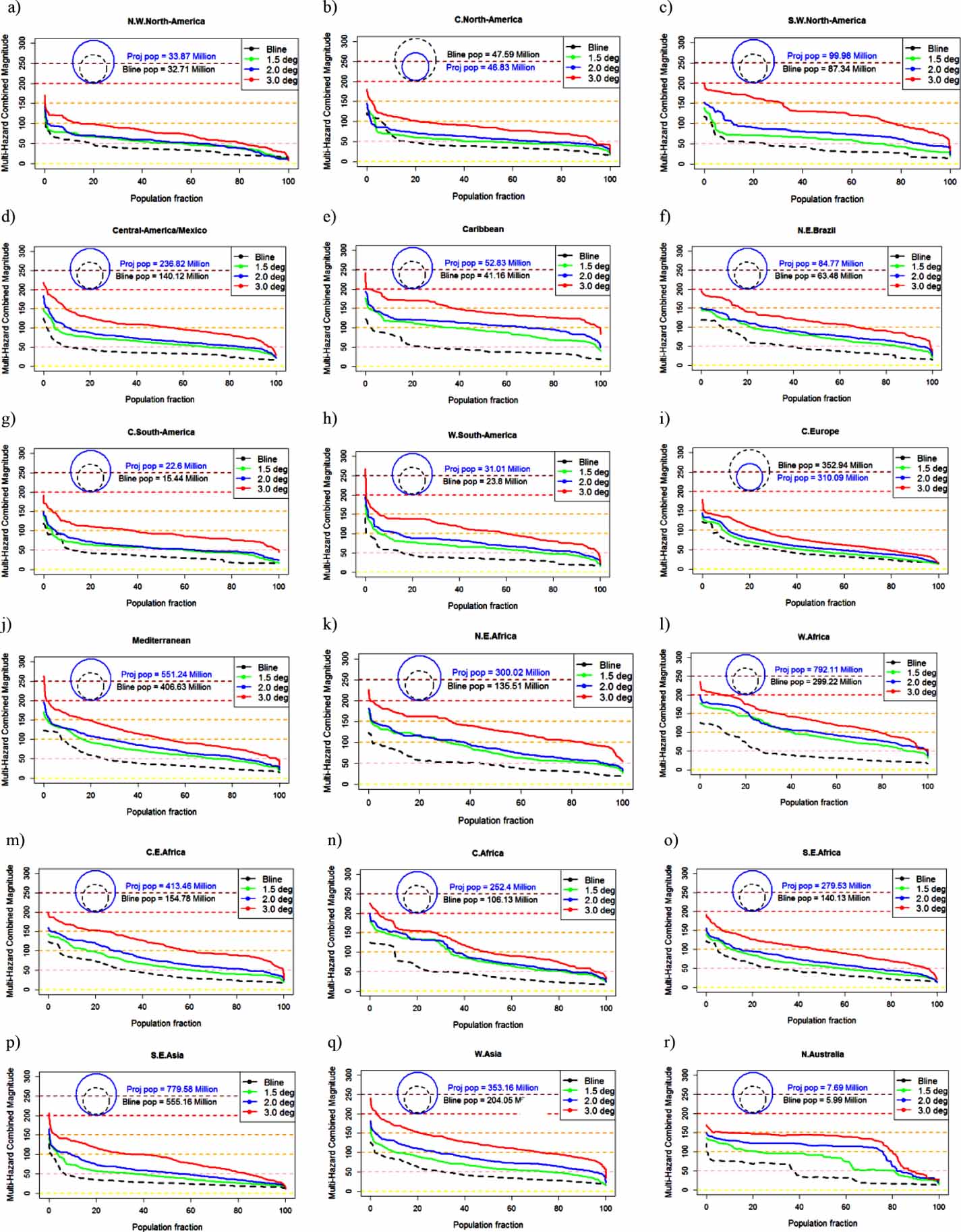
We then combine the multi-hazard analysis with projections in population growth to assess the relative distribution of the population exposed to different magnitude levels of the combined hazards for each scenario (in figure 2 results for selected regions). Each scenario includes 30 years of data for each grid-cell (see methods): these values are averaged (model change, in terms of 25th and 75th percentile—interquartile range, available in figure S2) and ranked with respect to the population distribution within each region. This enables the visualization of how the multi-hazard magnitude is spatially distributed with respect to the population in the region. Regions included in figures 2(a)–(r) were selected based on the overall magnitude reached in a normalized scale 0–300 (full list in figure S2). In each of the regions, roughly 20% of the population is expected to experience the highest values of multi-hazard magnitude under all scenarios. This means that about 20% of the population in each of the hotspot regions is exposed to the highest multi-hazard magnitude levels reached in the populated portion of the specific region, as non-populated grid-cells were excluded from this analysis (figure 2). North Australia stands as an exception, as the multi-hazard magnitude is distributed homogenously within about 40% of the population in the baseline, and 70% in the 3 °C scenarios (figure 2(r)). In some regions, the increase in population exposure is driven by both the increase in multi-hazard magnitude and the increase in population. This is particularly true in areas where demographic growth will be significant in the coming decades, as in North-East, Central-East and West Africa, and South-East Asia (figures 2(i)–(m), (p)). Taking West Africa as an example, in the baseline scenario 100% of the population (∼300 million people) is expected to be on average exposed to a multi-hazard magnitude larger than 25 (interquartile range 0–40 in figure S2), while the most exposed 10% (∼30 million people) to a value above 100 (75–135). In a 3 °C GWL scenario, 100% of the population (projected to increase from ∼300 to ∼790 million) would be exposed to a multi-hazard average magnitude greater than 50 (15–70), while the most exposed 10% (∼79 million people) to a magnitude of about 200 (165–250). More in general, the increase of the multi-hazard exposure between 2 and 3 °C is considerably higher than between 1.5 and 2 °C scenarios. In particular, in Africa and the Caribbean, a warming of 2 °C could double the baseline values of the multi-hazard, and a warming of 3 °C triple them for all population shares (figure 2). In the most populated areas of Northern Australia, about 50% of the population is expected to be exposed to a threefold increase in magnitude of the multi-hazard for all the scenarios (figure 2(r)) mainly due to the increasing droughts and heatwaves.

Figure 2. Share of the population exposed to different magnitude levels of the multi-hazard (combined 30-years average magnitude normalized to a 0–300 scale) for the reference and global warming levels by region. A full list of graphs is available in the supplementary material (figure S2). Population for the baseline and future scenarios is also displayed to provide an indication of the absolute values corresponding to each of the percent shares. The colour of the background dotted level-lines follows the 'Multi-Hazard Magnitude' colour scale plotted in figures 1(a) and (c).
Download figure:
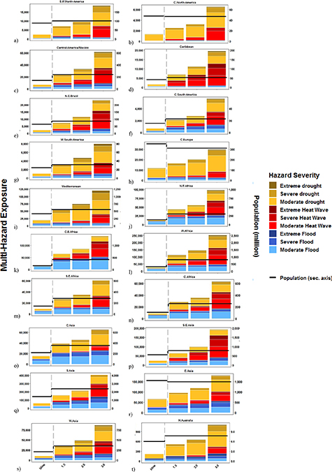
Standard image High-resolution imageThe comparison of the spatial distribution of the population and the combined hazard magnitude (figure 2) does not indicate how often the population will experience such hydro-meteorological events. Therefore, we stratify each hazard according to moderate, severe and extreme levels of severity (more info in the Methods) and we multiply the population by the hazards' frequencies under reference and warming level scenarios (hotspot regions in figure 3, full list in figure S3). These estimates provide an indication of the change in frequency of the events in relation to the potentially harmed population. Not surprisingly, population exposed to more frequent floods, heatwaves and droughts increase with respect to the reference period. While the overall number of flood events remains rather constant across the warming scenarios, the number of droughts and heatwaves is expected to rise substantially in the majority of the most populated regions. This is particularly the case for moderate and less severe episodes of droughts and heatwaves. Yet, even if the frequency of floods remains rather constant, their magnitude rises in all scenarios. This implies that the current flood defence infrastructure could be insufficient to contain future trends in the most developed countries, and more frequent disruptions in the least developed world. In particular, the flood share is estimated to increase in Asia, particularly in the Central (+100% in a 1.5 °C, +120% in a 2 °C, +130% in a 3 °C with respect to the reference scenario), Southern (+300%, +350%, +500%, respectively), and Eastern (+20%, +30%, +100%) portions of the Asian continent, especially when considering severe and extreme floods (figures 3(o), (q), and (r)). Beside changes in magnitude of the flood hazard, this is driven by the projected population increase in flood prone areas.
Figure 3. Population exposure to the three severity levels (moderate to extreme corresponding to lighter to darker colours) of the three hazards (flood-blues, heatwaves-reds, and drought-browns) for the three warming levels (Baseline, 1.5, 2, and 3 degrees increase in GWL). Black lines show the population change (in million, on the right axis) between 2010 (baseline) and 2050 (projection). On the left axis the Multi-Hazard Exposure level, here defined as Exp = Pop*Haz (population times hazard frequency). A full list of graphs is available in the supplementary material (figure S3).
Download figure:
Standard image High-resolution image
The rise in multi-hazard exposure over the Mediterranean Region (+120% in a 1.5 °C, +200% in a 2 °C, +400% in a 3 °C with respect to the reference scenario), North-East and West Africa (with similar increases of about +200%, +300%, +700%, respectively), and Central America (+200%, +300%, +00%) results from the combination of changes in both the hazards frequency and population exposed (figures 3(i), (j), (l), and (c)).
The change in exposure in South and South-East Asia (+150%, +270%, +500%), on the other hand, is mainly driven by the high population growth (+900 million people) likely concentrated in areas subject to hazards increasing at a relatively lower pace (figures 3(p) and (q)). Even in areas where population is projected to decrease, as in the case of Central Europe (−42 million), exposure is expected to increase (+50%, +100%, +200%) due to more intense and frequent hydro-meteorological hazards (figures 2(i) and 3(h)).
Few studies in the literature investigated the impact of the combination of multiple climate hazards (Piontek et al 2014, Forzieri et al 2016, Mora et al 2018, Byers et al 2018, Harrington and Otto 2018, Arnell et al 2019, Aghakouchak et al 2020, Batibeniz et al 2020). Although, the results presented in this study identify hotspot areas overlapping with other recent studies, the scope of this analysis is to test the concurrent evolution of multiple-hazard combinations with population trends. This goal was achieved with no consideration of the implications for the overall risk that are determined by the vulnerability of the human socio-ecosystem (Byers et al 2018, Arnell et al 2019). The evolution of the hydro-meteorological hazards estimated in our 1.5 and 2 degree warming are in line, and expand with one additional scenario, with the findings of the Half a degree Additional warming, Prognosis and Projected Impacts (HAPPI) project estimations (Mitchell et al 2017, Madakumbura et al 2019) that offered the quantitative assessments summarized in the IPCC SR15 (IPCC 2018). With respect to this project, the value that our study adds to the literature attains to the quantification of the combined effects of trends in multiple hazards occurring in the same temporal and spatial dimensions.
3. Conclusion
This analysis investigates to what extent limiting global warming to 1.5 and 2 °C, as for the Paris Agreement temperature targets, would substantially decrease the share of global population exposed to three widespread hydro-meteorological hazards—droughts, heatwaves, and floods—against a 3 °C warming scenario. We find that keeping temperature increase below 2 °C would reduce the share of global population exposed to the combined extreme hydro-meteorological events by more than 50%, in Africa, Asia and in the Americas, and by about 40% in Europe and Oceania. Additional efforts to limit it to 1.5 °C would further reduce the exposure by about an additional 10%–30% in all the areas considered. Globally, respect to a 3 °C, keeping the temperature increase below 2 °C would allow to keep more than 900 million people below a multi-hazard magnitude of 100 (0.9 vs 1.89 billion), 1.4 billion in the case of 1.5 °C (0.49 vs 1.89). Although this analysis is affected by several limitations, as the lack of consideration for vulnerability or the impossibility to analyse the consequences of events occurring simultaneously or sequentially at the same place, these results provide a powerful indication of the benefits that more ambitious mitigation policies would bring, and build a strong case for the Parties' NDCs to be revised in 2020 in line with the temperature targets of the Paris Agreement. Yet, raising the ambition of the adaptation component of NDCs will also be key. Resilience-developing activities are needed to avoid the most dangerous consequences of climate change on human and natural systems. While our study focused on the hazard and exposure components of risk, this knowledge can contribute to develop better informed multi-hazard risk management plans and thus reduce the likelihood that risk reduction efforts targeted on only one hazard might increase exposure and vulnerability to other hazards (IPCC IPCC, 2012bb). It therefore respond to the call of the Sendai Framework for 'an improved understanding of disaster risk in all its dimensions' and a 'multi-hazard approach to disaster risk reduction' (UN 2015, Anon 2019).
4. Methods
In this study, we assessed the combination of three hazards—flood, drought, and heatwave—and their main characteristics in terms of time, frequency, magnitude, and spatial distribution. Specifically, we relied on the projected indicators for heat-waves (Heat Wave Magnitude Index—HWMId) (Dosio et al 2018), drought conditions (Standardized Precipitation Evaporation Index—SPEI) (Naumann et al 2018), and river flood (Alfieri et al 2017) developed within the HELIX project. We refer to the original studies for the validation and calibration of the single hazard's indicators. The project brings together scientists from 16 organizations from all over the world to study the potential impacts of climate change under different GWL. Single hazard projections, estimated using seven different high resolution global climate models (Alfieri et al 2017) derived from the CMIP5 (Taylor et al 2012), were combined together and analysed in terms of magnitude and frequency. The multi-hazard analysis was then combined with projections in population growth from the shared socio-economic pathways 3 (Riahi et al 2017). Both socioeconomic and climate projections were assessed for the whole globe at a relatively high spatial resolution (half degree, corresponding to approximately 55 km at the equator). As in similar studies (IPCC IPCC, 2012aa), data is aggregated and visualized in macro geographical regions (Iturbide et al 2020—figure S1) by averaging the results over the region and accounting for the distribution of the hazards within the domain.
4.1. Climate data
The climate data used in this study are derived from the simulations performed by the Swedish Meteorological and Hydrological Institute (SMHI) using the EC-EARTH3-HR v3.1 earth system model (ESM) (Alfieri et al 2017, Dosio et al 2018, Naumann et al 2018). The SMHI ESM was forced using the outputs of seven different global circulation models (GCMs) belonging to the CMIP5 project (Taylor et al 2012) for the years 1971–2100, namely: IPSL-CM5A-LR, IPSL-CM5A-MR, GFDL-ESM2M, HadGEM2-ES, EC-EARTH, GISS-E2-H, and HadCM3LC (table S1). The seven models were selected to represent the full spectrum of change in terms of climate sensitivity and response (inter-model variability, wet vs dry) (Knutti et al 2013, Naumann et al 2018) among the full list of the CMIP5 models: the climate projections estimated for the IPCC AR5 report (IPCC 2013, Oppenheimer et al 2014). The years between 1971 and 2005 were forced using the historical output from the GCMs, while the future projections (2006–2100) were obtained using the RCP 8.5 scenario outputs of the climate models (Moss et al 2010, Vuuren et al 2011, Riahi et al 2011).
We defined the baseline reference period considering the 30 years between 1981 and 2010, while the warming threshold data were obtained by using the 30 years centred in the year by which the RCP 8.5 scenario of the specific climate model reaches the average warming level of, respectively, 1.5, 2, and 3 degrees with respect to the pre-industrial conditions following a methodology define 'time sampling' in James et al (2017) (table S2). The baseline covers a large part the period used in the referred studies (Alfieri et al 2017, Dosio et al 2018, Naumann et al 2018) to validate the single hazards with the observed data and was chosen here as reference to estimate the changes for the projected warming levels.
4.2. Population data
Population data were obtained from the SSP projections of population (Riahi et al 2017) provided by the International Institute for Applied System Analysis. The SSP original projections are available at country level. In order to get spatially explicit information, we used the downscaled data proposed by the Global Carbon Project (Murakami and Yamagata 2016) characterized by 0.5 degree resolution. To ensure consistency with the analysis of the climate threats, the scenario chosen for this study was the pessimistic number 3 'Fragmentation', a scenario compatible with high emissions characterizing the climate projections used (considering a RCP 8.5 scenario that do not reach the year 2100 in any of the combinations GCM-GWL) (Riahi et al 2017). Baseline population scenario refers to the years 1981–2010 data. In order to ensure the comparability between the different warming levels, the data for future population refer to the period centred in 2050 irrespectively of the level.
4.3. Hazard calculation
4.3.1. Heatwaves
Heatwaves were defined through the 'Heat Wave Magnitude Index daily' (HWMId) (Russo et al 2015), an index designed to account for both intensity and duration, successfully applied in recent research on the topic (Russo et al 2015, Forzieri et al 2016, Zampieri et al 2016, Ceccherini et al 2017, Dosio et al 2018). The index is calculated as the sum of the daily magnitude of all the days composing the heat-wave event. The methodology for its calculation and the comparison with alternative methodologies can be found in recent studies (Russo et al 2015, Dosio 2017, Dosio et al 2018). Shortly, as defined in Dosio et al (2018), the index indicates the maximum magnitude of the heatwaves occurring in a year. The heatwave is defined as the period of at three or more consecutive days with maximum temperature above the 90th percentile of a 31 d running window for the reference period (corresponding to 30 years). The index corresponds to the sum of the daily magnitude Md(Td) of all the consecutive days composing a heatwave (Dosio et al 2018). The magnitude is calculated (as in formula (1)) with respect to the 30 years interquartile range (being T30y25p and T30y75p, respectively, the 25th and 75th percentile of the yearly maximum temperature recorded over the reference 30 years period) for the specific location (Russo et al 2015).
As in previous studies (Dosio et al 2018), here the levels of intensity of the heatwave events (moderate, severe, extreme) have been identified with specific HWMId thresholds (20, 40, 80).
4.3.2. Drought
Drought calculation is based on the SPEI (Vicente-Serrano et al 2010). The index is calculated through the standardization of the difference (D) between precipitation (P) and reference evapotranspiration (ET0) in month i (formula (2)).

ET0 was calculated using the standard Penman-Monteith equation considering a standard reference crop (Burek et al 2013). The calculated difference values (D), representing a simple climatic water balance, were then fit in a statistical distribution (three parameters Log-Logistic distribution—formula (3)). The SPEI measures the deviation of the index for a running average of a certain number of months respect to the long term average conditions (considering a period of at least 30 years) (formulas (4) and (5)).

Being C0, C1, C2, d1, d2, d3 constant values, and P the probability of exceeding a determined D value (further details in Vicente-Serrano et al 2010)
For the scope of this analysis, a 12-month SPEI was considered suitable: SPEI with a 12 month accumulation period, in fact, is likely to capture longer term water deficits and hydrological droughts likely to affect agriculture, but also river discharge and groundwater recharge (Naumann et al 2018). Further information about the index are provided in the literature (Vicente-Serrano et al 2010, Vicente-Serrano and Beguería 2016, Naumann et al 2018), while the specific dataset used is publicly available (Naumann et al 2017). Drought severity were defined using the thresholds of −1, −2, −3, corresponding to moderate, severe, and extreme droughts, respectively.
4.3.3. Flood
Flood hazard is calculated using a global hydrological model (LisFlood (Van Der Knijff et al 2010, Burek et al 2013)) set up at 0.5 degree resolution (Alfieri et al 2017). A daily hydrological streamflow climatology at 0.1 degree resolution (∼11 km) was obtained by forcing the model with meteorological variables taken from an atmospheric reanalysis (Alfieri et al 2013) and then used to produce global inundation maps for six different return periods and spatial resolution of 30 arc-seconds (∼1 km at the equator) (Dottori et al 2016). Historical and projected flood events were identified using a Peak-Over-Threshold routine, which compares the return period of the peak flows with that of the flood protection levels at the grid-cell scale. The magnitude of the selected flood events is then linked to the corresponding inundation extent and used to estimate the exposed population. This methodology, fully described in a dedicated study (Alfieri et al 2017), allows to identify the number and magnitude of flood events for each of the climate scenarios produced. The selected events were stratified with respect to their magnitude and classified as moderate, severe and extreme floods, corresponding to the exceedance of return periods of 2, 10 and 100 years, respectively.
4.4. Normalization, aggregation and statistical analysis
Results of the seven simulations for each hazard were pooled and treated as a unique set of results for each 30 year period under consideration in each geographical region in the analysis. The change in magnitude of the three hazards in relation with the warming level was tested for statistical significance using three different statistical tests: 2-sample Kolmogorov–Smirnov test (Smirnov 1939, Engmann and Cousineau 2011); Anderson–Darling test (Scholz and Stephens 1987, Engmann and Cousineau 2011); and Student's t-test (Miller and Miller 1999). The hypothesis tests whether the two sets of data (the one related to the projected warming level and the baseline) were significantly different at 5% significance level. The most appropriate parametric or non-parametric test was selected by considering the results of the normality test (Shapiro–Wilk's test). Only after successfully passing these tests, the sample was marked as significant in figure 1. The tests were performed using the 'kSamples' package in R (Scholz and Zhu 2019).
The three hazard indicators of magnitude, i.e. SPEI, HWMId, and Flood return period, being calculated in the original studies in different scales, were normalized using a simple 'min-max' normalization procedure and rescaled in a 0–100 score, being 0 the minimum level of the hazard and 100 the maximum reached in the sample. Scores of the three hazards were summed up to obtain a multi-hazard overall score. The definition of multi-hazard we used is therefore the simple equally-weighted sum of the flood, heatwave, and drought normalized magnitudes with single hazards' magnitude scale 0–100, combined to get the multi-hazard scale of 0–300. Each of the hazards was assessed in order to account for their overall change in magnitude undergoing the statistical tests. The average magnitude values of the combined multi-hazards were used to make the estimations presented in figures 1 and 2. The uncertainty between the projections in the different models within the 30 years considered for each scenarios, was represented by plotting the interquartile range (25th and 75th percentile values) of the multi-hazard distribution (figure S2). After the change in magnitude was tested, hazard frequency was calculated for each class of severity and combined with the population to estimate the exposure level.
4.5. Calculation of the exposure
We quantified the number of moderate, severe and extreme events in each hazards at grid-cell level (0.5 degree) for each warming level scenario and each geographic region. The exposure of the population to the specific intensity category of the specific hazard was determined by multiplying the projected population by the frequency of a specific intensity event for each scenario and for each hazard severity. This number, which we define as multi-hazard exposure in figures 3 and S3, has no meaning in itself, but allows to monitor the degree of change of the combination of hazards and population dynamics for the different warming levels. In addition, the simple aggregation methodology is in line with the methodologies suggested by the IPCC (IPCC IPCC, 2012bb).
Acknowledgments
The research leading to these results has received funding from the European Union Seventh Framework Programme FP7/2007-2013 under Grant No. 603864 (HELIX: High-End cLimate Impacts and eXtremes; www.helixclimate.eu).
Data availability statement
The data that support the findings of this study are available upon reasonable request from the authors.
Author contribution
FF and AD designed the study; FF, AD, RS, LA, and GN performed the analysis; FF and EC wrote the paper with contribution from all the co-authors.
Data and code availability
The data that support the findings of this study are available from several databases listed in the Methods of the manuscript and the referred studies. Data are available from the authors on reasonable request and following data restrictions from the sources.
The main R functions and packages used in this study are provided in the Methods. Full R scripts are available from the authors upon reasonable request.
Footnotes
- 6
More details in the website (https://helixclimate.eu/).