

Abstract
We test an equation for the probability of heavy 24 h precipitation amounts Pr(X > x) as a function of the wet-day frequency and the wet-day mean precipitation. The expression was evaluated against 9817 daily rain gauge records world-wide and was subsequently used to derive mathematical expressions for different rainfall statistics in terms of the wet-day frequency and the wet-day mean precipitation. This framework comprised expressions for probabilities, mean, variance, and return-values. We differentiated these statistics with respect to time and compared them to trends in number of rainy days and the mean rainfall intensity based on 1875 rain gauge records with more than 50 years of valid data over the period 1961–2018. The results indicate that there has been a general increase in the probability of precipitation exceeding 50 mm/day. The main cause for this increase has been a boost in the intensity of the rain, but there were also some cases where it has been due to more rainy days. In some limited regions there has also been an increase in Pr(X > 50 mm/day) that coincided with a decrease in the number of rainy days. We also found a general increasing trend in the variance and the 10-year return-value over 1961–2018 due to increasing wet-day frequency and wet-day mean precipitation.
Export citation and abstract BibTeX RIS

Original content from this work may be used under the terms of the Creative Commons Attribution 3.0 licence. Any further distribution of this work must maintain attribution to the author(s) and the title of the work, journal citation and DOI.
1. Introduction
The term 'extreme' usually describes the largest (or smallest) variations of a measured quantity with a highly infrequent recurrence. Hence, extremes correspond to the 'far tails' of the statistical distribution and are commonly analysed within the framework of extreme value theory [1]. Usually the objective is to quantify the probability that the quantity exceeds a given limit Pr(X > x) or the n-year return-value which is an estimated threshold amount that is exceeded on average every n years. Here we use capital letter X to refer to a random variable and lower-case x when referring to a specific value or limit. It is the most extreme cases that usually have attracted the attention of the climate research community, and there has been a large number of studies on the link between climate and extreme precipitation, many of which discuss return values [2–9].
More moderate amounts have also been subject to analysis and modelling, and some early work with stochastic weather models date back to 1975 in which the bulk of daily rainfall amount was considered to be exponentially distributed [10]. It is important to study more intermediate precipitation amounts as well as the extremes, as moderately heavy precipitation also can have severe consequences. For instance, malaria outbreaks in Mozambique respond to the number of days typically receiving more than 50 mm in addition to the wet-day frequency fw (or the number of wet days), and the wet-day mean precipitation μ [11]. Furthermore, hazards such as mud/rock slides are more likely after heavy rainfall.
There has been a number of recent efforts where the probability density function (pdf) for daily precipitation has been described by a gamma distribution (see the appendix), although the degree to which a gamma distribution represents the daily rainfall has also been questioned [12]. A disadvantage of using the gamma distribution is that it is not always straight-forward to estimate its two parameters scale and shape [13], and it may be difficult to relate them to large-scale climate conditions. A simpler solution is to use the product between the fraction of wet days and an exponential distribution to describe the probability of heavy precipitation (see the appendix for the derivation of this expression) [14]:

where X is the 24 h precipitation amount and x is the threshold (e.g. 50 mm) defining heavy precipitation. The exponential distribution is a sub-set of the gamma distribution [10] and therefore has many of the same properties. It tends to under-estimate the higher percentiles of daily precipitation [15], but this bias appears to be constant for a given percentile or return-interval and can be adjusted for [16, 17]. Previous analysis of trends in the wet-day mean precipitation μ has been used to indicate trends in the upper percentiles [18] and this framework has provided a basis for downscaling the probability of heavy precipitation and the change in return-values [19, 20]. There are also studies suggesting that extreme daily rainfall amounts increase with higher temperature as indicated by the Clausius–Clapeyron relation [21, 22], however, the global mean precipitation amount is also constrained by the available energy [23]. The precipitation amounts are constrained by the availability of moisture, the specific humidity, which has been reported to correlate strongly with land surface temperature with increases broadly consistent with the Clausius–Clapeyron relation [24].
Our objective was to quantify changes in the rainfall statistics, here comprising the mean, variance, probability, and return-values. Before doing so, we evaluated equation (1) and derived the expressions for various rainfall statistics before using them as a yardstick to measure changes in the daily precipitation statistics over a large set of daily rain gauge data.
2. Methods and data
An advantage with equation (1) is its simplicity which makes it possible to derive a set of statistical properties based on two key parameters: the wet-day frequency fw and the wet-day mean precipitation μ. Both of these are easy to estimate and have clear physical interpretations. For instance, they can be used to express the mean precipitation  and are key parameters for both the percentile
  (for p > fw) and the return-value
  (see the appendix for proofs). These expressions, derived directly from equation (1), can be differentiated with respect to time in order to explain trends in probability, mean, variance and return-values. Hence the trend in these statistics can be related to trends in μ and fw.
We used daily rain gauge data from the Norwegian Meteorological Institute's climate database, the European Climate Assessment and Dataset (ECA&D) [25], the Global Historical Climate Network (GHCN) [26, 27] and daily station data from the CLARIS LPB dataset [28]. The combined data set included 9817 stations covering all continents and was used to test equation (1) by comparing the estimated probability to the observed frequency for the combination of individual year, site, and for five different thresholds (2 305 255 data points). Only a subset of 1875 sites with records longer than 50 years in the period 1961–2018 were included in the trend analysis (see the supporting material which is available online at stacks.iop.org/ERL/14/084017/mmedia, henceforth referred to as 'SM'). The mean and trends in annual fw and μ were estimated, using the threshold of 1 mm/day for a 'wet day'. Here we only looked at annually aggregated fw and μ and previous studies indicate that there usually is a mean seasonal cycle in both μ and fw [20, 29]. Nevertheless, equation (1) appears to describe the statistics for the different seasons [19].
The analysis was carried out in the R-environment [30] and made use of the esd-package [31]. An account of the processing and computations is provided in the SM in the form of an R-markdown script containing both R-code as well as figures and results.
3. Results
An overview of the rain gauge data suggested that the mean annual precipitation  totals vary geographically with greater amounts near the coast of Norway, the far northwestern USA, some Pacific islands, and southern US states where hurricane landfalls are fairly frequent (SM). The mean annual total precipitation was 796 mm for the subset of 1875 stations and the range of values was 25–3586 mm. Hence, the data represented a wide range of rainfall conditions. Regions with high wet-day mean precipitation μ included southern US states, the Mediterranean coast, parts of Argentina, and Pacific islands (the sample mean of μ was 7.21 mm/day with a range 2.8–18.6 mm/day) whereas the wet-day frequency fw was highest along the west coast of Norway and some Pacific islands. The mean frequency was 31%, with a minimum value of 1% and a maximum of 64%. The geographical rainfall characteristics corresponded well with the expected pattern, verifying that it gave a realistic picture of present precipitation climate.
For the selection of stations with records longer than 50 years, there was a general increase in the annual rainfall amount over the historical period (mean: 13 mm/year per decade; standard deviation: 23 mm/year per decade; range: −96 to 150 mm/year per decade), and further analysis suggested that this increase was due to a positive trend in μ (mean = 0.08 mm/day per decade; standard deviation 0.14 mm/day per decade; see SM) or increased or decreased wet-day frequency depending on the location (mean = 0%/decade; standard deviation = 1%/decade; see SM). For trends in the wet-day frequency, the general picture was a reduction in the subtropics and an increase at higher latitudes.
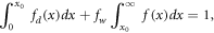
Figure 1 shows an example of equation (1) applied to daily rain gauge data from Bjørnholt near Oslo for which the equation was fitted by estimating the annual wet-day frequency fw and wet-day mean precipitation μ for each individual year. The estimated probability of precipitation closely followed the observed fraction of days with precipitation above the selected threshold (henceforth referred to as the 'empirical estimate') with a correlation of 0.85.
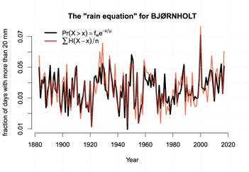
Figure 1. Example of equation (1) applied to the Bjørnholt rain gauge record near Oslo with high-quality observations. The black curve was computed from the annual wet-day frequency fw and wet-day mean precipitation μ with wet days being those with X > 1 mm/day. The black curve shows the estimate of Pr(X > 20 mm/day) obtained using equation (1) and the red line is the empirical frequency based on observations. We used the notation  which is the Heaviside function that returns 1 when X > x and 0 otherwise.
Download figure:
Standard image High-resolution imageTo test the framework more thoroughly, the same analysis as presented in figure 1 was repeated for different thresholds (10, 20, 30, 40, and 50 mm/day respectively) as well as for 9817 different stations world-wide. Figure 2 shows a comparison between calculated Pr(X > x) for each year and the observed annual frequency of events for all the five thresholds and all stations. The results suggested a high correlation between the estimated probability and the observed frequency (0.99).
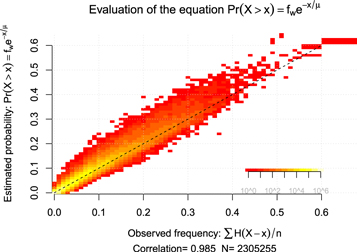
Figure 2. Heat map showing a comparison between the empirical (observed) annual frequency and estimated probability for daily precipitation exceeding 10, 20, 30, 40, and 50 mm. The colour scale shows the number of data points falling within each pixel and  is the Heaviside function. The data points represent different years combined from 9817 stations with available data. The colour scaling follows a logarithmic scale where yellow colour represents ∼105 points per pixel.
Download figure:
Standard image High-resolution imageWe tested the differential expressions for trends in both  (equation (B.5)) and Pr(X > 50 mm/day) (equation (B.3)) respectively, and our results verified that they corresponded to the sum of the terms representing the trends in fw and μ respectively (SM). The correlation was 1.00 for trend in
  and 0.97 for trend in Pr(X > 50 mm/day). These expressions provide a yardstick for assessing whether changes in the wet-day frequency fw, changes in the wet-day mean precipitation μ, or both are responsible for the observed trends in the rainfall statistics.
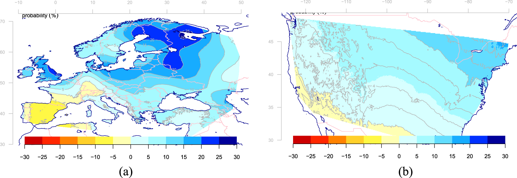
The mean value of the probability of heavy daily rainfall events Pr(X > 50 mm/day) was 0.1%, ranging from 0 to 1.6%. The highest values of Pr(X > 50 mm/day) were found over the southern states of the US, the Mediterranean coast, the west-coast of Norway, some Pacific islands, and the northeastern coast of Australia and corresponded to regions with high  and μ. Our analysis of the trends in Pr(X > 50 mm/day) suggested that heavy precipitation has increased over the period 1961–2018 at most locations with observations longer than 50 years. Figure 3 shows maps over Europe and the USA where the density of rain gauge data was relatively high, and both these regions were dominated by increasing Pr(X > 50 mm/day). The mean relative rate of change
  for the sample was 7.7%/decade and there has been an increase in Pr(X > 50 mm/day) at 76% of the 1875 sites included in this study with more than 50 years of data over the period 1961–2018 (figure 4). A majority of the rain gauge records (76%) indicated an increase in Pr(X > 50 mm/day) over 1961–2018, and most of these (95%) coincided with an increase in μ. For 72% of the records with increasing Pr(X > 50 mm/day), there had also been an increase in fw. The trend analysis also suggested that an increase in Pr(X > 50 mm/day) has taken place despite a decrease in μ for 5% of these cases and for 28% of the cases despite a decreasing number of rainy days. The trend analysis also indicated that the increase in the probability of heavy precipitation has been more strongly driven by the increase in μ than the increase in fw (SM).

Figure 3. The geographical distribution of the trends in probability of receiving more than 50 mm/day over 1961–2018. The units are %/decade in relative terms with respect to the 1961–2018 mean Pr(X > 50) for each respective rain gauge record, and the maps show gridded results based on the same kriging method as in [17].
Download figure:
Standard image High-resolution image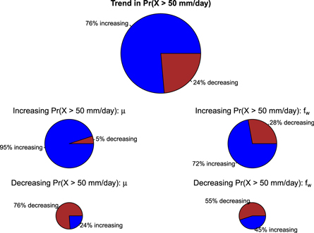
Figure 4. A summary of the trends in the probability of receiving more than 50 mm/day and the association with increases and decreases in μ and fw.
Download figure:
Standard image High-resolution imageTo further test the proposed framework, we compared estimates from the expression for the ten-year return-values  (equation (B.9)) with the empirical estimates, the threshold above which there was one observed event per decade on average. The empirical estimates were crude with wide error bars, but with a high volume of data, it was possible to discern a pattern. Figure 5 shows a scatter plot comparing the empirical estimates of the 10-year return-value for 1875 stations and the return-value estimate based on equation (1); a correlation of 0.86 suggests that it is possible to get an approximate estimate of the 10-year return value for daily precipitation based on fw and μ. One question is the minimum length of the series required to get good estimates for fw and μ, and if the rain gauge series is stationary, then we would expect fw and μ to converge to their true values. However, the rainfall data is not stationary, as cumulative estimates for fw suggests (SM), and xτ is expected to change overtime with trends in fw and μ. The results also showed a low bias that increased with higher rainfall amounts. We used a regression analysis to estimate a scaling factor for bias-adjustment:
  with best-fit
  (SM). The bias depended on the return-interval in a similar fashion as an increasing divergence found in the upper percentiles of daily rainfall amounts and the exponential distribution [16, 17]. We repeated the analysis for a set of return-intervals
 ![$[{\tau }_{1},{\tau }_{2},\,...{\tau }_{10}]$](https://content.cld.iop.org/journals/1748-9326/14/8/084017/revision2/erlab2bb2ieqn14.gif) , and found that the scaling factors increased monotonically from 1.25 for a one-year-event to 1.40 for a 10-year-event (table 1). The scaling-factors closely follow a straight line if plotted on a log-x-axis and it is perhaps possible to extrapolate their values to longer return-intervals (SM). The regression constant β0 did not show a clear dependency with timescale, and was of the order 3.9–4.7 mm/day and small compared to the return-values themselves (25–200 mm/day). This systematic bias is consistent with a previous comparison against corresponding return-values provided by general extreme value distribution (GEV) [32] and the proposition that the exponential distribution has a thinner tail than the precipitation [15].
, and found that the scaling factors increased monotonically from 1.25 for a one-year-event to 1.40 for a 10-year-event (table 1). The scaling-factors closely follow a straight line if plotted on a log-x-axis and it is perhaps possible to extrapolate their values to longer return-intervals (SM). The regression constant β0 did not show a clear dependency with timescale, and was of the order 3.9–4.7 mm/day and small compared to the return-values themselves (25–200 mm/day). This systematic bias is consistent with a previous comparison against corresponding return-values provided by general extreme value distribution (GEV) [32] and the proposition that the exponential distribution has a thinner tail than the precipitation [15].
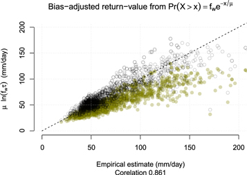
Figure 5. Comparison between calculations of the 10-year return-value based on  and corresponding empirical estimates from the observations. The black circles show bias-adjusted estimates that have been scaled by a factor of 1.4. The return-values were estimated for 1875 sites.
Download figure:
Standard image High-resolution imageTable 1.
Offset and scaling factor for bias-adjusting return-value estimates for return-intervals in the range of 1–10 years based on  . A best-fit of the correction-factor β1 to the log of the return-interval based on linear regression was:
 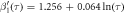 .
.
| Return-interval (years) | 1 | 2 | 3 | 4 | 5 | 6 | 7 | 8 | 9 | 10 |
|---|---|---|---|---|---|---|---|---|---|---|
| Offset (mm/day) | −4.2 | −4.2 | −4.6 | −4.5 | −4.7 | −4.5 | −4.4 | −4.1 | −3.9 | −3.9 |
| Scaling-factor | 1.25 | 1.30 | 1.33 | 1.35 | 1.36 | 1.37 | 1.38 | 1.39 | 1.39 | 1.40 |
Both trends in μ and fw have an effect on the 10-year-return-period x10, and in most cases (79%), there was an increase in both which resulted in higher values (SM). The mean estimate for the sample of 1875 sites was 0.6 mm/day per decade and spanned −5.2–6.9 mm/day per decade (not bias-adjusted), where 21% of sites were associated with a decrease in x10. Estimates of the proportional change (equation (B.11)) suggested a mean increase of 5% per decade in terms of the 1961–2018 mean, but with a very large range (−75%–94%) due to a number of outliers. For the majority of sites, the estimated proportional change in x10 was within the −10–+20% per decade range. According to the first derivative of  (appendix), changes in fw are expected to have a stronger effect on the proportional change in the return-value for the longer return-intervals whereas μ has the same effect on all timescales.
We also found increasing trends in σ2 for 79% of the sites (SM) which means that the rainfall has become more variable over the 1961–2018 period. The trends in the rainfall statistics derived from equation (1) were also consistent with the ratio of the number of record-breaking events to the number expected for time series of the same length but with identical and independently distributed (iid) data [33, 34] (SM). Our analysis indicated that there was on average 20% more cases with record-breaking rainfall than we would expect if the climate was stationary.
4. Discussion
The simple framework based on equation (1) implies that the parameters fw and μ provide information about both statistical characteristics and trends in daily rainfall. The trends in Pr(X > 50 mm/day) presented in figure 3(b) share a rough common geographical pattern with previous trend estimates of the frequency of very wet days (the 95th percentile of wet-day amounts over 1901–1978) over the period 1979–2013 [35], however, the results presented here also indicate more pronounced increases. These results differ in terms of interval and the quantity as we used an estimate based on equation (1) with a fixed threshold of 50 mm/day as opposed to the frequency of days exceeding an upper percentile. The framework, which included a number of expressions derived for a number of different rainfall statistics, was evaluated and verified against a large set of observations. While equation (1) is suitable for the bulk of the rainfall distribution including moderate extremes, it is not expected to perform well for the far tail of the 24 h rainfall distribution because it does not have a heavy tailed distribution [15]. It nevertheless provides a simple 'rule-of-the-thumb' number for moderate (10-year) return-values after systematic biases are adjusted for. This framework may be particularly useful for relatively short records as long as fw and μ can be reliably estimated.
The gamma and mixed distributions are more advanced and may provide a more accurate description than the exponential distribution, but the latter is both simpler and more practical and may serve as a benchmark for more advanced data models. It is difficult to obtain an expression from more sophisticated theory that expresses the trends in probability, variance, and return-values in terms of straight-forward quantities such as fw and μ. Extreme value theory (EVT) is usually based on block maxima (GEV) and peak-over-threshold (General Pareto distribution), but one limitation for EVT is that the sampling strategy on which it is based does not take into account the possibility of a changing sample size, e.g. when the number of rainy days per year increases or decreases. It is straightforward to demonstrate through a simple Monte-Carlo test that block maximum values associated with a stationary pdf tend to increase with sample size (SM), but the question is whether the estimated return-values are sensitive to this effect. The simple framework presented here showed that a trend in fw, and hence the sample size, may affect the estimation of both the probability of heavy rains and the return values. Moreover, EVT usually assumes stationary statistics whereas the framework presented here is suited for both varying fw and non-stationary statistics.
Our simple framework may benefit impact studies. The geographical distribution of some of the statistics presented here, such as Pr(X > x), σ2 and xτ, may correlate with the locations of impacts such as soil erosion, earth slides, vegetation, and how often crop failure vary. The different aspects of the rain statistics reflect different phenomena which vary with region and season [20]. One example is the high values for σ2 in the southern US states where tropical cyclones make landfall and produce substantial amounts of rainfall (SM). The variability may also be a result of more persistent events of rainfall and drought. In this case, σ2 does not give any indication about the temporal nature of the precipitation or whether the variance is due to changing regimes. It is likely, however, that changes in σ2 reflect a change in the local cloud climatology.
The simple framework presented here is particularly interesting for empirical-statistical downscaling if dependencies to large-scale ambient conditions and teleconnections can be used to project local fw and μ and hence risks associated with rainfall. For instance, El Niño Southern Oscillation influences the number of wet days over Australia, and equation (1) can be used to estimate approximately how this teleconnection affects the likelihood of heavy precipitation and hence give an indicator for the risk of flooding [36]. Results from previous efforts suggest that fw and μ are influenced by the mean sea-level pressure (SLP) and surface air temperature (SAT) respectively [19], but only part of the variations in μ has been attributed to SAT. These results also suggest that biases in SLP and temperature in global climate models will lead to errors in simulated extreme precipitation.
There may be several physical explanations for an increase in extreme rainfall with a stronger greenhouse effect and associated global warming. Higher surface temperatures lead to higher rates of evaporation and a more rapid turnover in the hydrological cycle. A change in the hydrological cycle is expected to affect the vertical energy flow and the atmospheric over-turning [37], and more intense rainfall is also often associated with higher cloud tops [38]. In addition, a decrease in the global area with daily rainfall implies a general decrease in fw and increase in μ [39]. Here figure 2 presented a heat map for a set of different thresholds to show that equation (1) works for a range of different thresholds. We leave more detailed analysis for different thresholds to future work.
5. Conclusions
Our analysis of a large set of daily rain gauge records indicates that heavy 24 h precipitation has become more frequent over the 1961–2018 period. The historical increase in the probability for heavy 24 h precipitation amounts has mainly been driven by increased wet-day mean precipitation and to a lesser extent by more days with precipitation. In some locations, heavy precipitation has become more likely over time in spite of a reduced frequency of the rainy days, suggesting a trend towards more droughts which are interrupted by more violent rainfall. There were also some cases where the probability of heavy precipitation has been driven by more frequent rainy days. We also show that trends in the wet-day mean precipitation and wet-day frequency have shifted the 10-year return-values for 24 h precipitation to higher levels.
Acknowledgments
This work was supported by the Norwegian Meteorological Institute and the KlimaDigital project (Norwegian Research Council grant: 281059).
Appendix A.: The gamma distribution
A common framework for daily precipitation is the gamma distribution and the equation describing its pdf is
which is specified by the two parameters 'scale' (α = k) and 'shape' (β = 1/θ) [10, 40–45].
Appendix B.: Mathematical proofs
Daily precipitation data were sorted into wet (X > x0 = 1 mm/day) and dry days, where the precipitation statistics were characterised by the annual wet-day mean μ and the annual wet-day frequency fw.
B.1. The exponential distribution
For rainy days, the 24 h precipitation is approximately represented by an exponential distribution:
for which the mean value is μ = 1/λ and variance σ2 = 1/λ2 = μ2. We were interested in the probability of exceeding a threshold Pr(X > x) rather than the probability of lesser precipitation Pr(X < x), hence 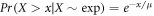 .
.
B.2. Dry and wet days
The probability of all possibilities adds up to one so that the integral for rainfall must be scaled by the fraction of the rainy days:
where we have defined X < x0 as a 'dry day' with negligible precipitation. The first integral is the fraction of dry days fd:
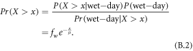
We can use Bayes theorem to derive equation (1) by considering the probability of a wet-day and the probability of exceeding the threshold on a wet day according to  . A is a wet day and Pr(A) = fw while Pr(B) = Pr(X > x). Since the probability is always one that it is a wet day given that the amounts exceeds the given threshold
  , the expression can be rephrased as:
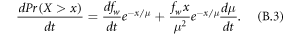
A change in the probability according to equation (B.2) is caused by a change in μ or fw and the effect of these two factors can be expressed through differentiation by parts (here x is a given level and not the subject for change):
B.3. The mean precipitation
A simple proof for the mean precipitation being the product between the wet-day frequency and the wet-day mean is:

A change in the mean precipitation is due to either a change in the frequency of wet-days or a change in the intensity.

B.4. Variance
The variance σ2 is more tricky to derive since the pdf is discontinuous. A formal expression for σ2 can be derived from an exponential distribution with a lower threshold x0 based on ![$E{[{X}^{2}]-E[X]}^{2}$](https://content.cld.iop.org/journals/1748-9326/14/8/084017/revision2/erlab2bb2ieqn22.gif) and the integration of the pdf [13, 46] as in:
and the integration of the pdf [13, 46] as in:
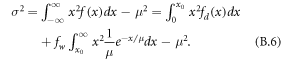
We take 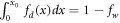 and assume that
 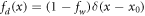 where δ is the Dirac delta function so that
  . Hence the right hand side of equation (B.6) can be written as:
Some of the terms are zero, as  ,
,  . α is a scaling factor, and the solution to this expression is within the range (x0 = 0, fw = 1) and (
 , fw = 0). The former gives σ2 = μ2, just as for the exponential distribution. The other gives σ2 = α − μ2 = 0, and α = μ2. Hence, we have the following expression for the variance:

The trend in the variance in 24 h precipitation can be expressed as
B.5. Return-values
The rain equation can be used to estimate return values associated with the return interval τ by taking Pr(X > x) = 1/τ, taking the logarithm of both sides of equation (1), and rearranging the terms:

The return value is related to the percentiles  and τ = 1/(1−p). We can also differentiate equation (B.9) with respect to time to express changes in the return values as a function of trends in fw and μ (using
  ):
):

We can calculate the proportional change δx/x, and after dividing by  on both sides of the equation. After some rearranging and cancellations, the expression for the proportional change in the return-value for a given return-interval τ is: