

Abstract
Drought-induced tree mortality has recently received considerable attention. Questions have arisen over the necessary intensity and duration thresholds of droughts that are sufficient to trigger rapid forest declines. The values of such tipping points leading to forest declines due to drought are presently unknown. In this study, we have evaluated the potential relationship between the level of tree growth and concurrent drought conditions with data of the tree growth-related ring width index (RWI) of the two dominant conifer species (Pinus edulis and Pinus ponderosa) in the Southwestern United States (SWUS) and the meteorological drought-related standardized precipitation evapotranspiration index (SPEI). In this effort, we determined the binned averages of RWI and the 11 month SPEI within the month of July within each bin of 30 of RWI in the range of 0–3000. We found a significant correlation between the binned averages of RWI and SPEI at the regional-scale under dryer conditions. The tipping point of forest declines to drought is predicted by the regression model as SPEItp = −1.64 and RWItp = 0, that is, persistence of the water deficit (11 month) with intensity of −1.64 leading to negligible growth for the conifer species. When climate conditions are wetter, the correlation between the binned averages of RWI and SPEI is weaker which we believe is most likely due to soil water and atmospheric moisture levels no longer being the dominant factor limiting tree growth. We also illustrate a potential application of the derived tipping point (SPEItp = −1.64) through an examination of the 2002 extreme drought event in the SWUS conifer forest regions. Distinguished differences in remote-sensing based NDVI anomalies were found between the two regions partitioned by the derived tipping point.
Export citation and abstract BibTeX RIS

Content from this work may be used under the terms of the Creative Commons Attribution 3.0 licence. Any further distribution of this work must maintain attribution to the author(s) and the title of the work, journal citation and DOI.
1. Introduction
The significant carbon sink that the world's forests represent plays a substantial role in balancing global carbon budget as well as influencing fluxes within other related reservoirs. However, the world's forests are being lost at a relatively rapid rate, as consequences of direct deforestation and climate-driven forest degradation (Contreras-Hermosilla 2000, Lambin et al 2003, Bonan 2008). The climate-driven forest declines are widely expected to increase in a warming world (Allen et al 2010, Zhao and Running 2010, Williams et al 2013, Wei et al 2014). Physically, this is because hot air can hold more water vapor, increasing atmospheric evaporative demand and duration between consecutive precipitation events (likely increasing severity of floods and droughts). Ecologically, trees suffer heat stresses and potential water deprivation by heat-driven drought as temperature approaches and surpasses certain levels, resulting in drought-induced mortalities. Widespread tree mortality induced by recent heat waves and droughts has been documented (Van Mantgem et al 2009, Allen et al 2010). This warmer climate-induced tree mortality is of concern because it may play a key role in a climate-carbon positive feedback system. Both modeling (Williams et al 2013) and observations (Yi et al 2010) have demonstrated that as temperature is above a certain threshold values, terrestrial carbon uptake is limited by relative water availability. Recent climate data show that more than half of the land surface is drying and the aerial extent which is experiencing this negative moisture balance is expanding with the warming climate (Yi et al 2014). A deduction from the above modeling and FLUXNET data re-analysis is that the rate of atmospheric CO2 transfer to land is expected to decrease, thus, resulting in further warming and drying. Drought-induced tree mortality has been shown to greatly reduce terrestrial carbon uptake (Zhao and Running 2010). However, the relationship between tree mortality and drought is reported to be more complex than that between grassland production and drought (Yi et al 2012). This is thought to be mainly due to the greater ability of trees to access water sources at greater depths leading to lower sensitivity to moisture levels in shallow soil horizons. Therefore, quantitative determination of what level of available moisture is sufficient to induce drought-related tree mortality is challenging and critical to understanding on the potential positive feedback to greater global warming.
Several lines of efforts have recently been made to quantify potential relationships between large-scale tree mortality and climate conditions by: (1) examining correlations between tree abundance in basal areas experiencing extreme drought conditions (e.g. Floyd et al 2009); (2) identifying response time-scales of forest to drought conditions (e.g. Vicente-Serrano et al 2013); (3) empirical-based predictions of tree-ring growth width as functions of warm-season vapor-pressure deficits and cold-season precipitation at regional-scales (Williams et al 2013) or as a function of Palmer drought severity indices (PDSI) (Ogle et al 2000); (4) using both empirical and process-based models to examine the responses of trees to droughts (McDowell et al 2013), and (5) site-specific ecophysiological studies, such as Breshears et al (2008), in which predawn water potential was measured before and during severe drought over more than a decade and associated with mortality of pinyon pine. Another approach is comparison of growth history between trees that died during drought and trees that lived, such as Macalady and Bugmann (2014) for pinyon pine and Kane and Kolb (2014) for montane conifers in the Southwestern US (SWUS). Most of these efforts have focused on coniferous forest of the SWUS primarily due to findings that tree mortality rates in SWUS have rapidly increased in recent decades with the warming climate (Van Mantgem et al 2009, Williams et al 2013) and the coniferous forest in these semiarid regions are usually highly resistant to drought (Vicente-Serrano et al 2013). No doubt, all these studies have advanced knowledge of forest decline to drought. However, using easily observed meteorological variables in combination with trees' physiological variables to predict possible drought-induced mortality is rare (Anderegg et al 2013). Here, we are looking for a relationship between a meteorological drought index and tree growth rate, by which the tipping point of tree mortality can be predicted.
Drought-induced tree mortality or dieback could occur when trees face extreme water deficits that exceed their ability to cope and acclimate. In this study, we considered the extreme water deficits where trees cease to grow as tipping point, below which the available water cannot meet the base level to maintain vitality and tree mortality or dieback could occur. With the aim to translate meteorological drought index into tipping point that triggers possible tree mortality, we hypothesize that the tipping point (i.e. threshold level of drought) can be determined by the monotonic dependence of tree growth on a drought index due to tree growth declines with increasing drought intensity under dryer conditions. Due to a relative abundance of documented tree growth-related ring width index (RWI) data for the SWUS, a better understanding of forest responses to drought can be expected. We use the extensive data sets of RWI of two dominant conifer species (Pinus edulis (PIED) and Pinus ponderosa (PIPO)) in the region to test our hypothesis. Tree-ring growth results from the interrelationships that exist between metabolism of carbon and plant hydraulics (McDowell et al 2011). For individual trees, ring widths are the end-product of these mechanisms and are expressively sensitive to moisture fluctuations (Liu et al 2013, Vicente-Serrano et al 2013). Thus, tree-ring is of key significance in drought reconstructions (Cook et al 1999, Stahle et al 2000). In further reference to drought-induced tree mortality, trees that died during droughts largely had lower pre-drought growth rates than those which survived. Thus, variation in tree-ring widths during the preceding 10–15 year time period can be used to aptly predict the likelihood of drought-induced mortality (Ogle et al 2000). In addition, ring width can be used for building models of growth-based mortality risk and assessing growth relationships to climate and competition (Macalady et al 2014). Tree growth is the balance of photosynthetic gains and respiratory losses in carbon (Amthor 1984). Under water-stress conditions, trees continuously regulate water use, via many mechanisms, including stomatal closure, leaf shedding and avoiding cavitation of xylem, resulting in rates of water production from respiration roughly equating to those of consumption due to photosynthesis, so as to delay forest mortality during drought (Huntingford et al 2000, Anderegg et al 2012). Such modulations lead to gradually inhibition in radial growth (Zweifel et al 2006).
Which drought index is most appropriate to develop an understanding of coniferous tree ring growth in response to dryer conditions across the SWUS? A number of drought indices have been produced for monitoring or assessing the spatial patterns and temporal trends of droughts (Du Pisani et al 1998, Heim 2002, Keyantash and Dracup 2002, Mezősi et al 2014), including (i) the PDSI (Palmer 1965, Dai 2011a, 2011b) that is based on a soil water balance equation; (ii) the standardized precipitation index (McKee et al 1993) that is based on a precipitation probabilistic approach; (iii) dryness (Budyko 1969, Zhou et al 2008, Yi et al 2010, 2013) that is based on annual energy and water budgets; (iv) forest drought-stress index derived from tree-ring data which is influenced by warm-season vapor-pressure deficit and cold-season precipitation (Williams et al 2013); and (v) the standardized precipitation evapotranspiration index (SPEI) indicates deviation from the average water balance (precipitation minus potential evapotranspiration) (Vicente-Serrano et al 2010). Here, we use the SPEI as a drought variable for data analysis because the SPEI data are available for different time-scales representing the cumulative water balance over the previous n months and also incorporates the effects of temperature on drought severity (Beguería et al 2013, Vicente-Serrano et al 2013). Time-scale is critical to assess the time-scales to which tree-ring growths are most sensitive to drought conditions especially to the persistence of water deficits.
2. Data and method
This study focuses on two dominant conifer species, PIED and PIPO in the SWUS (Arizona, New Mexico, Colorado, and Utah). The SWUS experienced a comparatively moderate to severe drought event in 2002, with record or near-record precipitation deficits throughout the region (Cook et al 2004). This event provides us with a natural experiment from which we can develop an understanding how such forest responds to severe droughts.
2.1. Data
2.1.1. Tree-ring
A total of 116 standard chronologies from the International Tree-Ring Data Bank (www.ncdc.noaa.gov/paleo/treering.html), representing two dominant conifer species, PIED and PIPO, served as the examined population in this study. The high density data were drawn from 116 sites for the conifers whose average age is 400 years and average elevation of their base is 2220 meters. Each chronology represents the average growth of several trees (22 samples per site) of the same species growing at the same site (supplementary table1, available at stacks.iop.org/ERL/10/024011/mmedia). The standard chronologies were created with the Program AutoRegressive STANdardization, by detrending and indexing (standardizing) from tree-ring measurement series, then applying a robust estimation of the mean value function to remove effects of endogenous stand disturbances (Cook 1985). The RWI value of 1000 represents mean growth values while value of 0 represents no growth. The mean length of the chronologies used was 80 years.
2.1.2. SPEI
Monthly data of SPEI with different time-scales at a spatial resolution of 0.5° were used to quantify meteorological drought conditions from 1901 to 2002. Different SPEI time-scales (1–24 month) represent cumulative water balance ranging from relatively short to long terms (e.g. SPEI obtained for time-scale of 24 month represents the cumulative water balance over the previous 24 months). These monthly data of SPEI with different time-scales were obtained from the SPEI website (http://sac.csic.es/spei/database.html), which is based on monthly precipitation and potential evapotranspiration values drawn from the Climatic Research Unit of the University of East Anglia. Since SPEI values have been found to be sensitive to global warming and are comparable in time and space and across time-scales, they can thus be utilized to quantify climatic anomalies in terms of intensity as well as temporal and spatial extents (Vicente-Serrano et al 2010, 2013).
2.1.3. NDVI
The NDVI dataset derived from July 1981 to December 2002 which were evaluated in this study were obtained from the Global Inventory Monitoring and Modeling Systems (GIMMS) group at the Laboratory for Terrestrial Physics (Tucker et al 2005). This particular dataset has a spatial resolution of 1/12° and temporal resolution of 15 day and has been widely used for monitoring global vegetation conditions (Wu et al 2014). A post-processing satellite drift correction was applied to the dataset to remove artifacts due to the orbital drift and changes in the Sun-target-sensor geometry (Pinzon et al 2005). This dataset is more sensitive to water vapor in the atmosphere as a result of the AVHRR's wide spectral bands (Brown et al 2006). An increase in atmospheric or soil water vapor results in a lower NDVI signal, which can be interpreted as an actual change if no correction is applied (Pinheiro et al 2004). The maximum value composite (MVC) method (Holben 1986) should lessen these artifacts. The MVC approach was applied to the original GIMMS 15 day NDVI composite data, which spanned 30 years from January 1982 to December 2002, to aggregate monthly data to reduce the influence from clouds in subsequent analysis.
2.2. Time-scale test and binned average
2.2.1. Time-scale test
For each year of a site, there is a single RWI value. However, there are 288 (12 × 24) different values of SPEI for each year because each month has 24 different values of SPEI over the time-scale spectrum (i = 1, 2,..., 24 months), indicating cumulative water balance ranging from short to long term. Thus SPEI data can be expressed herein as SPEIi,j (j = January,..., December). The objective of this effort is to locate which SPEI among 288 different values can serve as a better drought index for tree-ring growth. For instance, a site has n year RWI data, as well as each SPEIi,j (j = January,..., December) has n year data. Pearson correlation coefficient between RWI and each SPEIi,j can be calculated. Thus, we obtained 288 Pearson correlation coefficients for each site, which can be expressed as a matrix of 12 by 24. We obtained 116 such matrixes for the 116 tree-ring chronology sites. To determine the calendar month and time-scale (1–24 month) which best characterizes the generality of pattern of drought's influences on tree growth over the region, the 116 matrixes were averaged into a new matrix to represent the pattern at the regional-scale (figure 1). Among the subject population of 288 SPEI values, the SPEI which has a strongest correlation with RWI is the month of July with a duration of 11 months. Figure 1 also indicates that the cumulative water balance in winter and fall substantially contributes to drought condition in next year. This finding can alternatively derived from fact that the correlation between RWI and SPEI of June is the highest at durations of 9 months, SPEI of May at 8 months durations, and SPEI of April at 7 months durations. Based on figure 1, the SPEI of July with an 11 months duration will be used as drought index in this analysis.
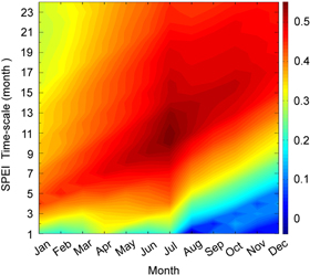
Figure 1. The distribution of mean Pearson correlation coefficients between RWI and SPEIi,j (i=1,2,...,24 months; jth month) from January to December over 116 chronology sites in the SWUS region. For each site, the Pearson coefficients can be expressed as a matrix of 12 months by 24 time-scales. We obtained 116 such matrixes for the 116 tree-ring chronology sites. To determine the calendar month and time-scale (1–24 month) which best characterizes the generality of pattern of drought's influences on tree growth over the region, the 116 matrixes were averaged into a new matrix to represent the pattern at the regional-scale. Among the subject population of 288 SPEI values, the RWI which has a strongest correlation with SPEI is that for the month of July with a duration of 11 months. Therefore, SPEI11,Jul is selected to use as a drought index in this analysis.
Download figure:
Standard image High-resolution image2.2.2. Binned averages
In order to properly represent the generality of relationships between tree growth and drought conditions over the region, 'binned average analysis' was carried out to minimize the uncertainty induced by spatial heterogeneity (difference in topography, soil property and forest density etc) that randomly affect tree growth among the 116 sites (de Toledo et al 2011, Peterman et al 2013, Williams et al 2013). Binned averages of RWI and SPEI were determined within each bin of 30 of RWI in the range of 0–3000 (approximately the maximum RWI). Thus, near 100 binned averages of RWI and SPEI were obtained through this method. Subsequently statistical population in each binned averages was examined. Binned averages with number of samples less than ten were excluded as they would increase statistical errors when analyzing the relationship between tree growth and drought conditions. Ultimately 72 binned averages of RWI and SPEI were valid in the study.
3. Empirical model
The relationship between the binned average RWI and SPEI is shown in figure 2. Two piecewise regressions separately by a breakpoint SPEIup = 0.35. Under dryer condition (SPEI < SPEIup), the piecewise regression is given by

where RWI represents the tree growth and SPEI11,Jul represents the drought condition quantified by water deficits over the previous 11 months accumulated up to July. The breakpoint SPEIup is the upper boundary beyond which tree growth is less limited by water stress. The result shows that, under dryer conditions, 99% variation of tree growth can be explained by SPEI11,Jul at regional scale. According to mechanisms of hydraulic failure and carbon starvation evaluated in the literature (Brodribb and Cochard 2009, Anderegg et al 2012, McDowell et al 2013), trees continuously regulate carbohydrate and hydraulic dynamics under water stress via stomatal closure, which minimizes hydraulic failure, causing photosynthetic carbon uptake to decline to low levels till respiration is proportional to photosynthesis (Huntingford et al 2000, McDowell et al 2008). Such controls result in zero net growth, exhibiting as RWI = 0, and increases risks of mortality of the subject conifer as ultimately stored carbonhydrates would be depleted during the protracted drought, or these resources couldn't be transported among tissues (Sala et al 2010). Therefore, drought conditions corresponding to an RWI being equal to zero is the theoretical tipping point at the species-level. The tipping point of tree growth decline to drought is predicted by the regression model as SPEItp = −1.64 and RWItp = 0. It suggests that conifer trees cease positive net growth when SPEI11,Jul approaches −1.64, which is the apparent tipping point for tree growth at regional scale.
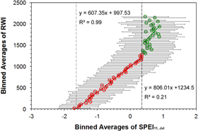
Figure 2. Relationship between binned averages of RWI and SPEI11,Jul SPEI11,Jul is the value of SPEI in July with time scale of 11 months, which accounts for water balance over the previous 11 months accumulated up to July. The circles are binned averages of RWI and SPEI11,Jul within every 30 bins of RWI in the range of 0–3000. The total of 116 standard RWI chronologies were from the International Tree-Ring Data Bank (www.ncdc.noaa.gov/paleo/treering.html), representing two dominant conifer species, Pinus edulis and Pinus ponderosa. RWI standard deviation bar in each bin were marked vertically, while SPEI standard deviation bar in each bin was marked horizontally. The SPEI11,Jul binned averages with statistical population less than ten were excluded as they would increase statistical errors when analyzing the relationship between tree growth and drought conditions. Ultimately 72 binned averages of RWI and SPEI were valid in the study. Two segmented regressions were conducted seperately: circles in red indicate dryer condition (SPEI < SPEIup = 0.35) and circles in green indicate wetter condition (SPEI > SPEIup). Under dryer condition, tipping point of drought (SPEItp = −1.64) was deduced from equation (1). SPEIup is the upper boundary beyond which tree growth is less limited by water stress.
Download figure:
Standard image High-resolution imageWhen climate conditions are wetter (i.e., SPEI > SPEIup), the piecewise regression is given by

Although the slope of regression (2) is higher under wet condition than that of regression (1) under dry condition, the correlation in regression (2) is much weaker than in regression (1), only 21% variation of tree growth can be explained by SPEI11,Jul.
4. Application
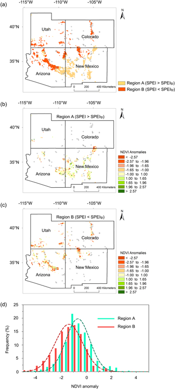
Since SPEItp was derived from physiological data at the species-level, it is necessary to verify whether it is applicable to forest ecosystem-level from the perspective of remote sensing. To execute this, an analysis of the severe drought in 2002 which occurred in the SWUS region was performed to compare the differences of forest responses to drought under two conditions: one with a severity less than the tipping point (SPEI > SPEItp) and conversely one with a greater severity than the tipping point (SPEI < SPEItp). Conifer forest regions (PIED and PIPO dominated) are defined herein as the distribution map of the general forest cover types from United States Department of Agriculture Forest Service (http://nationalatlas.gov/atlasftp.html), with a spatial resolution of 1 km. This map is derived from satellite imagery, ground-truthed by field observations and refined with ancillary data from digital elevation models as well as expert knowledge. There are about 70% RWI chronology sites locate in the range of 25 km of the conifer forest regions. Therefore, it is appropriate to use the region for further verification of whether the SPEItp (species-level) is applicable at the ecosystem-level.
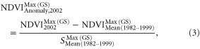
The conifer forest regions were partitioned into two regions, designated regions A and B, by the relative tipping point of SPEItp (figure 3(a)).The two regions represent the two drought conditions. Region A is characterized with lower severity of drought than the tipping point (SPEI > SPEItp) while region B is characterized with higher severity of drought than the tipping point (SPEI < SPEItp). Comparisons between the differences in responses to drought under the two relatively different drought conditions were made to verify if the SPEItp can serve as a tipping point at ecosystem-level. The responses of the subject forest to drought were quantified through use of standardized anomalies of GIMMS NDVI which served to evaluate potential changes in forest activity. In the process, NDVI in 1982–1999 is utilized to represent the normal condition of forest activity in the pre-drought periods. The standardized anomalies NDVI in the drought year of 2002 were calculated pixel by pixel by
where  represents the optimum growth condition of forest activity in growing season from March to October in drought year of 2002,
  represents the average optimum growth condition of forest in growing seasons from March to October during the pre-drought time period,
  represents the standard deviation of the optimum growth condition of forest spanning the growing season from March to October in pre-drought periods. Pixels with NDVI anomalies in the range ±1 standard deviation (std.) are classified as showing no changes; pixels with NDVI anomalies less than −1 std. are classified as significantly declined and with NDVI anomalies greater than +1 std. classified as significantly increased.
Figure 3. Conifer forest responses to drought under two drought conditions in 2002: (a) division of drought areas of conifer forest in the SWUS by the tipping point of SPEItp = −1.64 into two regions: region A (SPEI > SPEItp) and region B (SPEI < SPEItp); (b) spatial distribution of NDVI anomalies in region A in 2002; (c) spatial distribution of NDVI anomalies in region B; and (d) NDVI anomalies probability distribution of regions A and B. The conifer forest regions marked by both red and yellow color in figure 3(a) were derived from the distribution map of general forest cover types from United States Department of Agriculture Forest Service (http://nationalatlas.gov/atlasftp.html) with a spatial resolution of 1 km. 116 RWI chronology sites used in this analysis are marked with cross symbols. 70% of these sites were located in the range of 25 km of the conifer forest regions. NDVI anomalies were calculated by formula (3) pixel by pixel. Forest activity in region A was independent of NDVI anomalies less than −1std. in figure 3(b), while most parts of region B significantly changed, with NDVI anomalies beyond −1std. in figure 3(c). Average NDVI anomaly in region A was −0.28, less than −1std., indicating that forest activity was least affected by drought, while average NDVI anomaly in region B was −1.22, beyond −1std., indicating that forest activity was seriously affected by drought.
Download figure:
Standard image High-resolution image
Spatial patterns of NDVI anomalies in 2002 under two drought conditions were analyzed. It clearly appears that most parts of region A are independent of NDVI anomalies less than −1std. (figure 3(b)); while most parts of region B have NDVI anomalies beyond −1std. (figure 3(c)).The statistical results show that the average NDVI anomaly in region A was −0.28, less than −1std., showing no changes, indicating that forest activity was less affected by drought when SPEI > SPEItp. However, average NDVI anomaly in region B was −1.22, which in absolute terms is greater than −1std., showing significantly declined from which it is responsible to infer that forest activity was seriously affected by drought when SPEI < SPEItp (figure 3(d)).
This study further carried out independent t- test to analyze differences in forest activity between regions A and B during pre-drought period (1982–2001) and drought year of 2002 respectively. In the pre-drought period, the mean difference of NDVI anomaly between regions A and B is −0.055 55 (p = 0.70), indicating no significant difference in forest activity between them. Therefore, it is reasonable to consider forest activity in region A is statistically equivalent with region B in the pre-drought period. However, in the drought year of 2002, NDVI anomaly of region B was significantly lower than that of region A, with mean difference being −0.939 10 (p < 0.0001), indicating that forest in region B was affected by drought even worse than region A (table1). In this case, drought condition is the only difference between region A (SPEI > SPEItp) and B (SPEI < SPEItp), from which it is possible to deduce that the SPEItp causes the significant difference in forest activity.
Table 1. Average NDVI anomaly comparison between regions A and B during pre-drought period and drought year of 2002a.
| A versus B | t | Df | Sig (two-tailed) | Mean difference | Std. error difference |
|---|---|---|---|---|---|
| Pre-drought | −0.378 | 38 | 0.707 | −0.055 55 | 0.146 91 |
| Drought | −13.679 | 1359 | 0.000 | −0.939 10 | 0.068 65 |
aNDVI anomalies were calculated by formula (3) pixel by pixel. Independent t- test was carried to compare the forest activity between regions A and B during the pre-drought period and drought year of 2002 respectively. During the pre-drought period, the difference between the two regions is not significant with mean difference of −0.055 55 (p = 0.707). During the drought year of 2002, forest activity in region B was significantly lower than that of region A with mean difference of −0.93910 (p < 0.0001).
5. Discussion
Based on the physiological mechanisms on trees growth, response patterns of conifer species (PIED and PIPO) to droughts in the SWUS were analyzed by physiological data RWI combining with meteorological drought index at a relatively coarse scale. More importantly, the tipping point of tree responses to drought at the species-level over the region has been discovered. McDowell et al (2013) has studied physiological mechanisms that is related to drought-induced tree mortality through multiple model-experiment framework. They believed that tree mortality was determined by time spent at extensive hydraulic failure or carbon starvation. Such a critical drought condition in duration and intensity has been deduced in our study, i.e. when drought sustains for duration of 11 months with intensity of −1.64, trees growth are expected to cease, leading to possible tree mortality.
In this study, patterns of response to drought at forest ecosystem-level under two drought conditions have been further examined from remote sensing perspective. The results shows that when drought severity exceeds the tipping point (i.e. SPEI < SPEItp), NDVI significantly decline with average NDVI anomaly less than −1std. (figure 3(c)), which is tightly tied to regional mortality (Breshears et al 2005). Also region B generally is coincide with the areas that experienced noticeable levels of tree mortality identified by aerial survey conducted by the US Forest Service (US Forest Service 2003). Therefore, region B generally denotes the area of forest with differential mortality. Therefore, the tipping point at species-level could be up-scaled to forest ecosystem-level, represented as physiological drought indicator for PIED and PIPO dominated forest. When drought severity exceeds the tipping point, differential forest mortality can be expected to occur, leading to damages in forest structure and consequently its function.
Although SPEItp was derived at the species-level, the application from remote sensing has already confirmed that SPEItp could be scaled to forest ecosystem-level, indicating that SPEItp is applicable for current studies on drought impacts. Therefore, the SPEItp can aptly serve as a criterion, along with climate models to study dynamic vegetation simulations under different climate change conditions, for a better understanding on forest response to potential climate change in an effort to mitigate adverse impacts.
In order to survive under water stress, trees decrease allocation to growth, leading to increases in susceptibility to other disturbances (e.g. biotic agents) (Breshears et al 2005, McDowell et al 2008, McDowell 2011, McDowell et al 2011). Recent studies indicate that ≥1 year of severe drought predisposes PIED to insect attacks and increases mortality (Gaylord et al 2013). Besides, increased temperatures can enhance the net damage due to tree pests indirectly, by encouraging pest reproduction and dispersal (Raffa et al 2008), which will increase risks of forest mortality. However, due to lack of available relevant data, we did not investigate potential effects of such biotic factors. Investigations of potential synergies between precipitation and other climate variables with biotic factors affecting forest activity is strongly encouraged from the results of this and other studies.
Due to different levels of missing climate data from observation stations for the long period of ∼80 years since 1901, SPEI time-series at 0.5° were used for this study. SPEI at this coarse scale might bring possible scale-effect-errors in analyzing relationship between tree growth and drought since the RWI chronologies were derived at stand-scale. However, with the higher density of the RWI chronologies, stable relationships were found between SPEI and RWI as Pearson correlation is above 0.5 for most sites (81.35%) independently of the SPEI time-scale and month of the year (supplementary table 2).
6. Conclusions
Determining the quantitative relationship of forest response to drought and subsequent revelation of the tipping point of these low precipitation conditions is crucial for an assessment of climate change impacts on a forest ecosystem. The results in this study indicated that a tree's RWI has a good statistical relationship with the climate drought index SPEI at 11 month time-scale in July (SPEI11,Jul), from which the tipping point of drought (SPEItp) that trees can endure can be deduced. This study's results specifically show that the tipping point (SPEItp) of PIED and PIPO is −1.64, that is, drought sustains for duration of 11 month with intensity of −1.64 might lead to differential mortality. As an indicator of ecosystem phenology, NDVI significantly declined in area where the SPEI < SPEItp, than that in area where SPEI > SPEItp, which illustrated that the tipping point of drought derived from RWI could be up-scaled to the ecosystem-level to assess possible impacts of climate change on forest ecosystem.
Acknowledgments
This work was supported by the Fund for Creative Research Groups of National Natural Science Foundation of China (No. 41321001), the National Basic Research Program of China (No. 2012CB955401), the New Century Excellent Talents in University (No. NCET−10-0251), US PSC-CUNY Award (PSC-CUNY-ENHC-44-83), and the International S&T Cooperation Program of China (Grant No. 2012DFG21710). CY is grateful to the International Meteorological Institute for support when he performed this work as Rossby Fellow. Our thanks also go to the two anonymous reviewers for their contribution to improve the manuscript.