

Abstract
Time series of visibility and aerosol optical thickness for the Netherlands have been constructed for 1956–2100 based on observations and aerosol mass scenarios. Aerosol optical thickness from 1956 to 2013 has been reconstructed by converting time series of visibility to visible extinction which in turn are converted to aerosol optical thickness using an appropriate scaling depth. The reconstruction compares closely with remote sensing observations of aerosol optical thickness between 1960 and 2013. It appears that aerosol optical thickness was relatively constant over the Netherlands in the years 1955–1985. After 1985, visibility has improved, while at the same time aerosol optical thickness has decreased. Based on aerosol emission scenarios for the Netherlands three aerosol types have been identified: (1) a constant background consisting of sea salt and mineral dust, (2) a hydrophilic anthropogenic inorganic mixture, and (3) a partly hydrophobic mixture of black carbon (BC) and organic aerosols (OAs). A reduction in overall aerosol concentration turns out to be the most influential factor in the reduction in aerosol optical thickness. But during 1956–1985, an upward trend in hydrophilic aerosols and associated upward trend in optical extinction has partly compensated the overall reduction in optical extinction due to the reduction in less hydrophilic BC and OAs. A constant optical thickness ensues. This feature highlights the influence of aerosol hygroscopicity on time-varying signatures of atmospheric optical properties. Within the hydrophilic inorganic aerosol mixture there is a gradual shift from sulfur-based (1956–1985) to a nitrogen-based water aerosol chemistry (1990 onwards) but always modulated by the continual input of sodium from sea salt. From 2013 to 2100, visibility is expected to continue its increase, while at the same time optical thickness is foreseen to continue to decrease. The contribution of the hydrophilic mixture to the aerosol optical thickness will increase from 30% to 35% in 1956 to more than 70% in 2100. At the same time the contribution of black and organic aerosols will decrease by more than 80%.
Export citation and abstract BibTeX RIS

Content from this work may be used under the terms of the Creative Commons Attribution 3.0 licence. Any further distribution of this work must maintain attribution to the author(s) and the title of the work, journal citation and DOI.
Corrections were made to this article on 26 January 2015. The correct version of the supplementary data was published.
1. Introduction
In studies of atmospheric turbidity the visibility, aerosol optical thickness and shortwave surface irradiance are linked parameters. Their binding agent is the visible extinction which is a measure of the amount of light being scattered out of the light path. Thus in order to reconstruct, or produce future scenarios of the optical parameters it is necessary to understand the physical phenomena controlling the extinction coefficient in such a manner that a satisfactory explanation of the time-dependent signatures of all three parameters can be obtained at the same time.
Over many parts of the Western world an increase in surface irradiance is observed, a phenomenon termed 'solar brightening' (see Wild 2009, for a review and an extensive bibliography). The consensus view is that after about 1985 a reduction in the emission of anthropogenic aerosols is responsible for causing a decrease in aerosol optical thickness. The brightening followed a prolonged period of decreasing shortwave irradiance, the period of so-called 'solar dimming'. In Western Europe, fogs (visibility less than 1 km) have been on the decline for more than 30 years which can similarly be attributed to a reduction in aerosol emissions (Vautard et al 2009). Yet, on closer examination there are inconsistencies between the records so that a uniformly decreasing aerosol concentration can not serve as a satisfying explanation. For example, the minimum in observed surface irradiance between 1985 and 1990 Wild et al (2005) would suggest a corresponding peak emission in anthropogenic aerosol and a peak in aerosol optical thickness. Yet, the continuous decline in the occurrence of fog over the same period during which such peaks are observed suggests a corresponding continuous decline in aerosol emission. The inconsistencies are indicative of the complexities involved in understanding the underlying physics.
One aspect in the debate on improving visibility which has not been sufficiently highlighted is the relative contribution of hydrophilic versus hydrophobic aerosols to visibility. Hydrophilic aerosols result in greater visibility impairment than hydrophobic aerosols because at high relative humidity (RH) hydrophilic aerosols attract more water than hydrophobic aerosols, so their surface area is larger and their capability to scatter light out of the direct path between object and observer is enhanced. Over the last 50 years the amount of aerosols as well as the composition of aerosols have changed significantly, so that it is important to understand what the impact of the changed aerosol composition is on visibility.
The purpose of this paper is to interpret the changing optical properties over the Netherlands in terms of changing aerosol mass and composition.
Aerosol optical thickness has been retrieved from visibility observations (1956–2013) over the Netherlands. An aerosol emission scenario (1956–2100) is used to distribute the total aerosol mass amongst individual species with individual hygroscopicities. Next, the visible extinction is calculated and deviations of the calculated extinction from the observed extinction are minimized by adjusting the input aerosol masses and their relative proportion. The procedure to obtain optical thickness from visibility bears resemblance to a recent study by Wu et al (2014) who applied a similar approach to China.
A framework is presented in which the relative importance of the aerosol concentration and the aerosol hygroscopicity in contributing to the time varying signatures of aerosol optical thickness and visibility from 1956 to 2100 is highlighted.
2. Methods
2.1. Visibility observations
In the Netherlands weather and climate observations are recorded at 42 stations. The majority of these stations date back to the 1970–1980s. However, a number of stations have a longer history. For this study we are particularly interested in long continuous records of visibility. Five stations were chosen, consisting of the five main climate stations (De Kooy, Vlissingen, De Bilt, Eelde and Maastricht). Together they form a good representation of the region (see figure S1 in the supplementary data, available at stacks.iop.org/ERL/10/015003/mmedia for additional information on the specific methods to measure visibility).
Here, four visibility classes are defined. The first class is 'fog', which is defined as a visibility of less than 1 km. This is the traditional definition and no further differentiation into moderate and dense fog is used. The second class is 'low visibility' with visibility restricted between 1 and 5 km. The third class is 'moderate visibility' with visibility between 5 and 10 km. Finally, the fourth class is 'good visibility' and applies to situations with a visibility larger than 10 km.
2.2. Conversion of visibility to aerosol optical thickness
Visibility (Vis) is defined as

where the Rayleigh scatter at the same wavelength is neglected.
The aerosol optical thickness δaer at 550 nm is given as

The scale height for aerosols (H) is assumed to be constant over time. Its value is adjusted so as to conform to the remote sensing observations. For every year, the time series of hourly visibility values is converted to visible extinction by solving equation (1) for  and averaged over the entire year. Then equation (2) is used to retrieve a time series of yearly averaged optical thickness. The scale height for aerosols has been adjusted until the time series agreed with observations and is taken to be 900 m (see S2).
2.3. Aerosol mass model
A long-term time reconstruction is made of aerosol composition valid for the center of the Netherlands (Cabauw, 52.0N, 4.9E, a site about 50 km inland located 22 km west-southwest from De Bilt). The historical part of the reconstruction (1950–2000) is based on the Community Atmospheric Model (CAM)-inventory by Lamarque et al (2010), while the projections for 2000–2100 are based on the aerosol emission scenario following the Representative Concentration Pathway 4.5 (RCP4.5, van Vuuren et al 2011). The combined data set we refer to as the CAM-inventory because we use for the scenario the aerosol composition simulated with the Lamarque et al. CAM chemistry-climate model using the RCP4.5 aerosol emissions. The CAM-inventory has been intended for use in climate model simulations within the framework of the Climate Model Intercomparison Program No. 5 (CMIP5) in support of the Intergovernmental Panel on Climate Change (IPCC) Fifth Assessment report (AR5).
The CAM-inventory has been calibrated for present-day conditions using observations of aerosol composition in the Netherlands (Matthijsen and Koelemeijer 2010, Wichink Kruit et al 2012) together with regional model simulations using the national operational Air Quality Lotos-Euros model (L-E model) (Schaap et al 2008). The aerosol composition, representative for the years 2007–2008, is taken from Matthijssen and Koelemeijer (2010). The anthropogenic component of annual country mean PM2.5 is largely composed of secondary inorganic aerosols (SIA, 46%) and total carbonaceous matter (TCM, 29%) with the remaining fraction dominated by the fine fractions of sea salt and dust. Total observed SIA is 6.7 μg m−3 and total observed TCM is 4.3 μg m−3.
An L-E model simulation for the year 2005 is used to split the observed SIA load into nitrate, ammonium and sulfate components representative for Cabauw. This yields SIA fractions representative for present-day relative amounts of nitrate (∼40%), ammonium (∼25%), and sulfate (∼35%). The TCM fractions for organic aerosol (OA) and black carbon (BC) from the L-E simulation are ∼60% and ∼40%, respectively.These values are close to the observed fractions given by Matthijssen and Koelemeijer (2010), which are representative fractions for the whole country of ∼70% and ∼30%, respectively. The split between the SIA and TCM components was taken from the observations and not from the L-E model because the L-E model is assumed better capable of simulating the individual fractions of SIA and TCM than the division of total particulate matter between SIA and TCM. The L-E model underestimates the present-day OA concentrations, mainly because of the complex formation of secondary OA. It remains difficult to adequately include this process in the simulations (e.g. Schaap et al 2008).
The CAM-inventory provides decadal mean concentrations of sulfate, OA and BC on a 2.5 × 1.9 (lon × lat) degrees model grid. Here the grid cell centered at 52.1N and 5.0E has been used. The CAM-inventory does not cover nitrate and ammonium. These components are added to the calibrated CAM sulfate component maintaining the L-E-derived SIA fractions of sulfate, nitrate and ammonium. Next to sulfate and the natural components sea salt and wind-blown dust, the CAM-inventory provides concentrations of OA and BC. The OA and BC components of CAM are further sub-divided into, respectively, hydrophobic fractions (OA1, BC1) and hydrophilic fractions (OA2, BC2). The 2000–2010 decadal mean hydrophobic and hydrophilic fractions of CAM are then used to subdivide the L-E derived OA and BC fractions. In CAM, for the 2000–2010 decade, the OA hydrophilic fraction is 58% and the BC hydrophilic fraction is 33%.
Table 1 provides the overview of the present-day calibrated CAM-aerosol components together with the observed and L-E-scaled concentrations of nitrate and ammonium as described above. The total anthropogenic aerosol hydrophilic mass (Mahp) is the sum of SIA, OA2, and BC2. Compared to the CAM aerosol components the sulfate component in 2005 is reduced by the calibration against observations with ∼40% (from 4.0 to 2.2 μg m−3) while TCM is increased by ∼50% (from 2.9 to 4.3 μg m−3). The total anthropogenic fraction of the hydrophilic mass in CAM (sulfate + OA2 + BC2) is increased by ∼60% (from 5.5 to 8.8 μg m−3), mainly through the addition of nitrate and ammonium which are missing components in the CAM-inventory.
Table 1. Aerosol mass for the CAM aerosol types after calibration and the additional nitrate and ammonium mass. The total anthropogenic aerosol hydrophilic mass for Cabauw representative for the year 2005 is the sum of SIA + OA2 + BC2.
| Aerosol component | Calibrated mass (μg m−3) | CAM-inventory (μg m−3) |
|---|---|---|
| SIA | 6.7 | 4.0 |
| Nitrate (NO3) | 2.9 | — |
| Ammonium (NH4) | 1.6 | — |
| Sulfate (SO4) | 2.2 | 4.0 |
| TCM | 4.3 | 2.9 |
| Organic Aerosol hydrophilic (OA2) | 1.7 | 1.0 |
| Organic Aerosol hydrophobic (OA1) | 1.3 | 0.7 |
| Black Carbon hydrophilic (BC2) | 0.4 | 0.4 |
| Black Carbon hydrophobic (BC1) | 0.9 | 0.8 |
| Total anthropogenic aerosol hydrophilic mass Mahp = SIA + OA2 + BC2 | 8.8 | 5.5 |
| Total anthropogenic aerosol mass | 11.0 | 6.9 |
The evolution of nitrate and ammonium is not provided by the CAM-inventory. Maximum nitrate and ammonium concentrations of 20% above their observed mass in ∼2005 have been assumed for the 1990s taking into account the decrease in precursor emissions since about 1995. A linear increase from very low concentrations in the 1950s to the peak in 1995 has been assumed. Future projections of nitrate and ammonium are uncertain and dependent on future choices with respect to agricultural practices for ammonium and policy implementation of further reductions in NOX emissions, mainly related to industry and traffic. A stabilization of the nitrate and ammonium concentrations since 2005 is assumed.
Only part of the highly soluble NaCl interacts with NH3, NO3 and SO4 (Manders et al 2009), therefore an unmixed NaCl group is defined and treated separately (see S3).
2.4. Aerosol chemical, physical and optical properties
The growth of aerosol with RH is dependent upon the hygroscopicity. Using the abbreviation DUS to denote mineral dust, the approach taken here is to make initially a separation between the aerosol group of (BC1, BC2, OA1, OA2, DUS) and the group (SO4, NH3, NO3, Na, Cl).
For the first group OA, and BC that are insoluble the value of the hygroscopicity κ is set at zero. The groups of soluble OA, BC consists of subspecies with unknown relative composition and the actual composition will affect their hygroscopicity (Massoli et al 2010, Chang et al 2010). It appears that κ = 0.4 is a reasonable approximation for both the soluble OA and BC species so as to balance the large proportion of insoluble OA and BC, yielding an average value of κ for the entire OA–BC group ranging from 0.1 to 0.3 (Duplissy et al 2011, McMeeking et al 2011).
Even though DUS is generally thought of insoluble or marginally soluble Herich et al (2009), Hatch et al (2008) suggest that DUS is often coated with soluble compounds due to mixing with anthropogenic aerosols. DUS can therefore interact in water chemistry processes to provide a partly soluble aerosol. Here the value κ = 0.1 is used to indicate its marginal solubility.
For the second group of relatively soluble aerosols (SO4, NH3, NO3, Na, Cl) no hygroscopicity can be assigned to individual cations or anions and they are assumed to interact. The interaction is simulated by means of the water chemistry model ISORROPIA (Nenes et al 1998, see S4). For the given composition a volume-weighted hygroscopicity is found to range from 0.65 to 0.75 which is comparable to the κ-values obtained from the individual aerosol species specified in ISORROPIA (see S4).
Size distributions are reconstructed using two assumptions: (1) the distributions conform to the (lognormal, two modes) shape of the distribution and the aerosol concentrations as observed during the EUCAARI—extended period (2008–2010) at the climate station of Cabauw using an SMPS probe (Asmi et al 2011) and (2) the shapes of the distributions do not change over time, only the total aerosol concentration. Under these two assumptions (plus small correction term, see S5) the mass per species can be calculated from the third moment of the lognormal distribution, or vice versa.
Mie-calculations were performed as a function of RH and of species and stored in tables to facilitate rapid access during the scaling calculations (see S6). For the mixture of dry inorganic aerosols it is assumed that they are purely scattering with an index of refraction of Na2SO4: md = (1.50–0.0i). For BC the consensus best value of md = (1.97–0.79i) is used (Bond et al 2013). For the group of soluble OA it has been suggested that most OAs only have absorptive capability in the UV part of the solar spectrum (Lund Myhre and Nielsen 2004). Brown carbon is viewed as a particular subspecies of OA and is an absorber of solar radiation at visible wavelengths (Andreae and Gelencsér 2006, Alexander et al 2008, Srinivas and Sarin 2013). In the absence of any precise information it is assumed that OA is purely scattering: md = (1.70–0.00i)). Also, a small imaginary part was given to mineral dust (DUS) (md = 1.50–0.01i). See (S7) for the impact of aerosol properties on visibility.
2.5. Scaling computed with measured extinction
Consider now the extinction of the aerosol species (σj) calculated at a base aerosol concentration (Nj), their respective hygroscopicities (kj), and their current aerosol concentrations (Ni,j). Here the index i refers to the yearly-mean aerosol concentration for the individual species j derived from the aerosol scenarios. The index j refers to the species. Then it follows that there should be agreement between the modelled and observed values of extinction via equation (1)

Here, σobs is the extinction computed from the visibility observations. Unfortunately, equation (3) has too many unknowns to arrive at a unique solution. The scaling choices will be discussed in section 3.
3. Results
3.1. Visibility
The results for the five stations in the Netherlands are plotted in the four panels of figure 1.

Figure 1. Visibility classes for the Netherlands. Red and black lines comprise the average of the five stations. Grey area is standard deviation over the five climate stations.
Download figure:
Standard image High-resolution imageFor each of the visibility classes, the number of hours occurring in a class was counted and the mean value and standard deviation (grey region) over the five stations were plotted.
Visibility improving with time is a consistent signature in all four plots. After 1970, there is a general decrease in the number of hours with visibility less than 1 km. The fog visibility class is the only one in which a fraction of the aerosol particles will activate to cloud droplets and the data presented here indicates that this class has been reduced by 50% in the last 47 years with a further (smaller) reduction expected until 2100. Yet, the class of low visibility shows an initial increase in the number of hours from 1956 onwards reaching a plateau between 1970 and 1985 after which it decreased again. Additionally, until 2013 there has been a 25% reduction in the number of hours in the class of moderate visibility, and, since the 1980s about 1500 h per year have been added to the class of high visibility. This amounts to almost 15% of the total of 8760 h available in a year of 365 days. In the years to come the class of high visibility is projected to grow at the expense of the two adjacent classes (see S8 for further details). Depending on the visibility class in which one is interested, different conclusions can be drawn about when the upward trends in visibility have started. If one is interested in extreme conditions such as fog, the situation has continually been improving since the early 1970s. Yet, the classes of higher visibility indicate the onset of improved visibility more than a decade later. One (partial) explanation of these differences is the non-linear behaviour of visibility with RH. The reduction in visibility is gradual from RH = 30% up to RH = 85%. However, from RH > 85% visibility rapidly deteriorates. Therefore, a uniform improvement in air quality which underlies most visibility studies will impact the different classes in different ways (see also S7 for a plot of visibility versus RH).
3.2. Aerosol optical thickness
Figure 2 shows the retrieval of De Bilt station. Here a three-point smoother is applied to facilitate comparison with the remote sensing observations. The remote sensing observations consist of ground-based retrievals for the period 1959–1971 at De Bilt (Frantzen 1977), ground-based retrievals from radiation equipment at Cabauw, and retrievals from the standard MODIS AQUA en TERRA data sets (Savchenko et al 2003). Despite some year-to-year variability there is good agreement between the data and the optical thickness retrieval. The fact that only a single scaling height could be used to achieve agreement between the retrieval and the different observations indicates that this is a robust result.
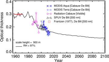
Figure 2. Optical thickness retrieval for De Bilt. The various data sources are centered in the region between Cabauw and De Bilt. Cabauw is the KNMI research station which is located at a distance of 22 km towards the southwest of De Bilt.
Download figure:
Standard image High-resolution image3.3. Aerosol mass model
The time series from the aerosol emission scenarios from European emission inventories from 1956 to 2100 of the eleven species at Cabauw are shown in figure 3.
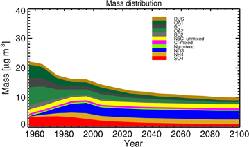
Figure 3. Estimates of the mass of the eleven aerosol species as determined from the aerosol emission reconstruction and scenarios from European emission inventories (1956–2100).
Download figure:
Standard image High-resolution imageThere is a strong reduction in BC and OA aerosols in the period 1955–1990. In the same period SO4 peaks around 1980 and then decreases, while the masses of NH3 and NO3 both increase. When observing the relative proportions of the various species it is apparent that the water chemistry in the Netherlands is undergoing a transition from a sulfur-based chemistry as was the case in 1960–1980 to a nitrogen-based chemistry from present day onwards until 2100. Overall there is a decrease in aerosol mass throughout the full 145-year period. Half of this decrease takes place in the first 55 years, the other half in the last 90 years.
3.4. Reconstruction/scenario 1956–2100
Based on the aerosol properties treated in Section 2.4 the grouping of aerosols can be further simplified into three. The first group comprises the natural aerosols consisting of NaCl-unmixed and DUS. They remain constant in time and their combined impact on visibility and extinction is constant throughout the entire period. This group is colour-coded as green in the figures to follow. The second group consists of the soluble inorganic mixture which includes the Na released from NaCl upon interaction with NO3, NH3 and SO4. As a fraction of the total mass this group is increasing rapidly, and will by the end of the period be the dominant aerosol group in the Netherlands. This group is colour-coded as blue. The last group consists of the marginally soluble and insoluble OA and BC combined. This is the group that has undergone the largest reduction in aerosol mass and it is colour-coded as brown.
There are two options to scale the modelled extinction to the observed extinction. Option 1 is defined by attributing all differences between the measured and modelled visible extinction to the group of highly soluble aerosols. Option 2 is defined by attributing all differences exclusively to the group of aerosols of low solubility. Most confidence is endowed to the specification of the group of inorganic soluble aerosols (blue coloured), as their time dependence is confirmed by local observations in the Netherlands. This means that option 2 can be considered the most plausible reconstruction option for the Netherlands and will be pursued here.
Figure 4 shows the reconstruction/scenario for the aerosol mass, number concentration and aerosol optical thickness. A three-point smoother was applied to the data in order to facilitate the separation in colour schemes. The red line indicates the unscaled original mass reconstruction/scenario (see S9 for the original scenario-plot in three colours). Assuming option 2, where any difference is owing to the low solubility aerosols, it appears that the total mass of BC and OA for the reconstruction is considerably higher than in the scenario, on the averaged roughly doubled. A factor of around 2 is used as a continuous scaling fraction for BC–OA after 2013 to allow for continuity between the scaling before 2013 and the scenario thereafter. Most reduction in mass, concentration and optical thickness occurs after 1985. The relative contributions of the various aerosol components to the optical thickness are different from the relative contributions of the mass and concentration. Even in the early period of 1956–1990 when BC–OA assumes at 70–80% of the total mass a dominant position in the aerosol grouping, the contribution of the inorganic mixture to the aerosol optical thickness is at 40–60% quite considerable. This means that the changing aerosol composition has a non-negligible impact on the evolution of aerosol optical thickness even though there is a reduction in BC–OA by 50% in the period 1956–2013. The overall hygroscopicity is increased from 0.3 to 0.4 over this period which again is mostly due to the increased importance of the soluble inorganic mixture in the aerosol composition. Interestingly, the values around 2000–2010 are very close to values of 0.4–0.5 as reported by Pringle et al (2010) in their estimates of κ for the region of the Netherlands derived from atmospheric chemistry model simulations.
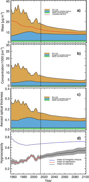
Figure 4. Reconstructions of (a) aerosol mass, (b) number concentration, (c) optical thickness and (d) hygroscopicity, averaged over the five climate stations.
Download figure:
Standard image High-resolution imageThere are considerable differences in aerosol mass, concentration and relative contribution to optical thickness by the different aerosol groups if option 1 (scaling with the group of highly soluble aerosols) were chosen. In that option, there are simply not as many aerosols needed to make up the difference in extinction because hydrophilic aerosols are more efficient in taking up water (thus reducing visibility). For option 1, this amounts to a 25% reduction in aerosol mass/concentration in the early part of the period (1960–1985) when compared to option 2. Furthermore, the contribution of these highly soluble aerosols to the overall optical thickness would have been double that of option 2. The implication is that the choice of scaling option is a sensitive factor in determining the relative contributions of aerosol mass and optical thickness.
3.5. Pathway
Since aerosol hygroscopicity and concentration are the dominant factors contributing to aerosol optical thickness and visibility they are plotted in a single plot of figure 5, both on a log scale.
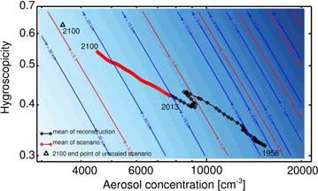
Figure 5. Reconstruction/scenario pathways.
Download figure:
Standard image High-resolution image
The essential point of this plot is to demonstrate that the change in aerosol composition implies that visibility has improved less than would be expected if it were based on a reduction in aerosol concentration while leaving the composition the same. This plot shows a number of isolines. The slanted straight red lines are isolines of equal optical thickness, the slanted blue lines are those of equal visibility. For this plot we chose the RH of 87% to compute the isolines. The reason for choosing a fixed value of RH is because optical thickness and visibility are both functions of RH, while in figure 5 the only two variables are aerosol concentration and hygroscopicity. Optical thickness (visibility) is increasing (decreasing) towards the upper right, the darker region of the plot. The isolines of the two variables are parallel to each other, as is to be expected based on the fact that one is the inverse of the other. Note that the individual points on this plot do not adhere exactly to the optical thickness values of figure 4 because in this figure, optical thickness and visibility are computed at a fixed RH, while the points in figure 4 are based on data obtained at all values of the RH as present in a year's worth of data. The reconstruction starts at 1956 in the lower right, and ends in 2013 in the middle. To facilitate comparison between pathways a 10-point smoother was applied on the data.
The general slant in the curve from lower right to upper left is an illustration of the importance of the hygroscopicity change in shaping the optical thickness time varying signature: during part of this period the mass of soluble inorganic matter increased while at the same time the relatively insoluble BC/OA aerosols decreased. While for the first group of aerosols visible extinction is increased due to their enhanced capability to take up water, for the second group visible extinction is decreased as this group is reduced in size. The optical thickness resulting from the simultaneous increase and decrease of the different aerosols is thus only slowly decreasing for the period 1956–1985 at the end of which it crosses the 10 km visibility isoline in figure 5. Thereafter, it more rapidly decreases until 2013 in accordance with the rapid reduction in BC/OA during that period. The rapid reduction in BC/OA combined with an increase in the soluble inorganic mixture results in a general increase in hygroscopicity so the general movement of the pathway trace is towards the upper left (i.e. towards the left to reflect a lower aerosol concentration, and towards the top to reflect increasing hygroscopicity). The pathway as indicated in figure 5 highlights its dependence on the relative strength in trends of the different aerosol types involved in shaping the optical thickness. This point is often overlooked in studies on trends in 20th century optical properties.
The pathway 2013–2100 is plotted, as derived from the aerosol mass scenario in figure 4. The plot indicates that future changes in visibility and optical thickness will not be as large as has been observed over the last 50 years (see also figure 1). The pathway for the period 2013–2100 shown by the trace in figure 5 has an identical scaling fraction for the BC–OA group as for the year 2013 to allow for a continuous transition towards the 2013–2100 scenario at the year 2013. However, for comparison purposes we included the 2100 end point of the unscaled pathway as the black triangle in the upper left. This illustrates the amount of uncertainty in simulating the pathway into the future.
4. Discussion and conclusions
We have presented a reconstruction/scenario pathway for visibility and aerosol optical thickness over the Netherlands. For the reconstruction of optical thickness, existing scenarios of aerosol mass and composition have been adjusted such that the measured extinction (from inverting visibility) matches those obtained from aerosol concentrations. This procedure led to a set of two aerosol reconstruction options of which the option of correcting the original mass scenarios for BC and OA is deemed to be the most realistic. Overall, the aerosol concentration is decreasing. It is found that the contribution of hydrophobic aerosols to the overall aerosol mass has strongly decreased over the last 57 years and will continue to do so in the ensuing 87 years. The group of soluble inorganic aerosols has increased initially as the total of NO3–SO4–NH3 aerosols reached a plateau around 1985 after which it decreased. The increase of this group of aerosols led to an increase in hygroscopicity of the entire mixture. Decreasing aerosol concentration and increasing hygroscopicity have an opposing influence on aerosol optical thickness, and on visibility. A plot showing aerosol concentration versus aerosol hygroscopicity was introduced which can trace the regional aerosol state as a function of time, a so-called pathway. The aerosol pathway in the Netherlands is one of decreasing aerosol concentration and of increasing hygroscopicity due to the continuous reductions in relatively insoluble BC and OA with respect to the rest of the aerosols. As such the observed reduction in aerosol optical thickness is not as large as it could have been in case the overall hygroscopicity of the combined aerosol groups would have remained constant instead.
There are two distinct sources of uncertainty that should be taken into account when interpreting our results. Firstly, the conversion of aerosol mass to concentration involves an informed decision on the precise shape of the size distribution. Although we followed the shapes of aerosol size spectra that were recorded in the Netherlands during the last years of the entire period, such information is not always present. Also, the further one goes back in time, the less likely is the chance that such information can be derived from increasingly sparse data sets. Trends in mean aerosol size due to changed composition or external factors such as changing land use can change the shape of the size spectra and thus would impact the aerosol concentration scenarios. The sensitivity of the aerosol concentration to changes in the shape of the total distribution has been investigated by changing the magnitude of the third (relatively large particle) mode by 50%. This means that the two smaller modes would have to adjust (by 20%) in order to fit the measured extinction.
Secondly, the choice on the most realistic/plausible reconstruction option depends to a large extent on whether the underlying aerosol scenarios are credible and/or verified by other data sources. In the case at hand, the most believable aerosol scenario is the estimated concentration of the soluble inorganic aerosol mass. In other words, the BC/OA mass is endowed with the least confidence. Allen et al (2013) indicate that none of the CMIP5 surface solar radiation computations agree with observations indicating that aerosol emission values are underestimated. Bond et al (2013) suggested that present estimates of BC in the 20th century could easily be doubled or tripled which supports our choice of scaling options. However, it is important to realize that the chosen scaling option has a large impact on the relative contributions of the individual aerosol groups to mass, concentration and optical thickness.
To conclude, this study suggests that there is considerable merit in further investigation of the importance of overall aerosol composition in the interpretation of turbidity observations. At present, shortwave irradiance has been excluded from our analysis due to the difficulty in discerning clear from cloudy signals. Nevertheless, the presence of long records of shortwave irradiance and visibility holds promise for more interpretative studies in the future.
Acknowledgments
The authors acknowledge the MODIS Science team and the GES DAAC MODIS Data Support Team for making MODIS data available to the user community.