Ground surface temperature and continental heat gain: uncertainties from underground

Hugo Beltrami; Gurpreet S Matharoo; Jason E Smerdon

doi:10.1088/1748-9326/10/1/014009

1. Introduction

Observed increases in global temperatures in the recent past have intensified research on the Earthʼs climate system and all its components, including the overall global energy budget (Pielke 2003, Hansen et al 2005, Levitus et al 2005, Beltrami et al 2006, Murphy et al 2009, Trenberth 2009, Hansen et al 2011, 2013, Stocker et al 2013). Detailed measurements of many climate variables and proxy indicators, as well as numerical models of the Earthʼs climate system, have been used to characterize the full range of variability of the climate system during multiple paleoclimatic intervals, including those in the Common Era (e.g. Coats et al 2013, Fernández-Donado et al 2013, Schmidt et al 2013, Phipps et al 2013). Because all proxy climatic indicators are a response to changes of a complex dynamical system, they are neither a direct measure of climate change nor represent an absolute response to a specific climate variable. Thus, they have varying spatial and temporal degrees of uncertainty. A comprehensive characterization of uncertainties in paleoclimatic data is therefore necessary to effectively use climate proxies to infer changes in a given climate variable.

Among independent paleoclimatic indicators, that is, an indicator that need not be calibrated with meteorological records, geothermal data have contributed significantly to the understanding of past climate during part of the Common Era, offering a different and complementary view of long-term, low-frequency temperature changes during the last few centuries at local, regional, hemispheric and global scales (e.g. Beltrami and Mareschal 1991, Beltrami et al 1992, Clauser and Huenges et al 1995, Šafanda et al 1997, Pollack and Huang 2000, Golovanova et al 2001, Majorowicz et al 2002, Roy et al 2002, Pollack et al 2006, 1998, Huang et al 2000, Harris and Chapman 2001, Beltrami 2002b, Beltrami et al 2002, Pollack and Smerdon 2004, Beltrami and Bourlon 2004, Beltrami et al 2006). Climate reconstructions from geothermal data assume that long-term surface air temperature (SAT) changes are coupled to long-term ground surface temperature (GST) changes, and that the long-term variability of the surface energy balance propagates by thermal conduction into the subsurface. There is support for long-term coupling between SAT and GST from direct evaluation (e.g. Smerdon et al 2006, Stieglitz and Smerdon 2007), and also from energy considerations as the continental heat gain estimated from subsurface temperatures (Beltrami 2002b, Beltrami et al 2006), differs little from the continental heat gain as estimated from meteorological data, for the last 50 years of the 20th century (Huang 2006).

The subsurface temperature anomaly as a function of depth is indicative of the temporal history of the heat exchange between ground and atmosphere, while the integral over depth of the subsurface temperature anomaly is proportional to the total heat absorbed or released by the ground. However, the thermal field of the subsurface is the response of a complex system at the surface and is sensitive to noise and uncertainties. The factors contributing to subsurface temperature anomalies and the associated uncertainties in the reconstruction of past surface temperatures and subsurface heat content changes are many and complex. These factors include land-use changes (deforestation in particular), non-conductive heat transfer effects such as soil freezing and thawing or advection due to ground water flow, and measurement uncertainties such as the depth and interval of temperature measurements in a given borehole and the precision of the measurement instrument. An important source of uncertainty is related to thermal noise from lithological variability, that is, high-frequency variation of the thermal properties of the heterogeneous subsurface. Also, previous climate events such as warming from the Last Glacial Cycle obscure the semi-equilibrium geothermal regime, and physically add a band of noise to the geothermal regime at all depths (Rath et al 2012, Beltrami et al 2014). Thus, it is crucial to obtain intervals of confidence for the models of GST histories inferred from borehole temperature profiles (BTPs), as these data have the potential to yield, among other things, information on the land component of the global energy balance of the climate system (Beltrami 2002a, Hansen et al 2005, 2011).

The International Heat Flow Commission (IHFC) borehole temperature database contains temperature profiles measured from the second half of the 20th century until the present. However, early BTP measurements were made for the purpose of estimating the heat emanating from the interior of the Earth, with an emphasis on the understanding of the thermal structure of the subsurface, and to obtain an estimate of the energy available for plate dynamics. Thus, the most common situation encountered in the BTP database is that of a large number of profiles measured with poor vertical sampling intervals (10 or 20 m intervals), which was sufficient for the objectives at that time. Modern BTP data are measured at higher sampling intervals, and these data are also suited for climatic inferences for which details of subsurface temperature variability are important. Nonetheless, because of the scarcity of BTPs, most of the data available have been used in previous analyses. Therefore, it is desirable to examine the potential effect that the data sampling interval and the depth range of the BTP section used to determine the quasi steady-state geothermal regime have on the the reconstructed GST histories and on the estimates of subsurface heat content.

Our focus is on estimating the uncertainties for the quasi-equilibrium geothermal gradient because it is the reference from which past GST changes are estimated. That is, the accuracy with which the geothermal gradient is determined is mapped directly onto the results of paleoclimate analyses regardless of the method of analysis. The semi-equilibrium geothermal gradient also represents the initial conditions—or magnitude of subsurface heat content, from which all estimates of ground heat storage, gains or losses, are measured, and hence its accuracy has direct implications for the results of the analyses of the role of continental energy in the overall energy budget of the climate system.

We estimate the variability expected for the long-term surface temperatures, heat-flow, and density for the IHFC dataset in the Northern Hemisphere arising from the uncertainties in the estimates of the quasi-steady-state geothermal gradient. We present the estimated uncertainties for the past 50 years of GST history, as well as uncertainties in the continental heat storage for the first 200 m of this region. Our efforts better constrain the plausible range in these two estimates based on a new characterization of uncertainties associated with the quantification of a fundamental background signal in all applications of borehole paleoclimatology.

2. Theoretical background

The temperature at a given depth in the Earthʼs subsurface is the superposition of all prior thermal contributions from above and below, i.e., the downward-propagating signal from changes in the surface energy balance and the upward propagating geothermal heat from the interior and from radioactive decay. For BTPs of less than 1000 m, the volumetric heat production, h, is often neglected. Assuming a homogeneous subsurface with constant thermal properties, the temperature at depth z, $T(z)$ , is thus determined by the superposition of the long-term surface temperature ${{T}_{0}}$ , the geothermal gradient ${{\Gamma }_{0}}$ and that of the temperature perturbation, ${{T}_{t}}(z)$ , caused by ground surface temperature variations (Carslaw and Jaeger 1959):

$\begin{eqnarray}&&T(z)={{T}_{0}}+{{\Gamma }_{0}}z+{{T}_{t}}(z).\end{eqnarray} \tag{ 1 }$

Because the energy contributions to the subsurface thermal profile from the Earthʼs interior are essentially constant on timescales of centuries to millennia, they can be removed by estimating a background linear-temperature increase with depth. The set of temperature departures from this quasi-equilibrium state are thus the temperature anomalies associated with the downward-propagating climate signal and are described by the one-dimensional diffusion equation (Carslaw and Jaeger 1959).

The shape of the subsurface temperature anomaly as a function of depth represents the history of the temporal changes of the upper boundary condition, that is, the history of the energy balance at the surface. The integral of the subsurface anomaly is proportional to the subsurface heat gain or loss from the subsurface. Typically, GST histories are inferred by inversion (Shen and Beck 1991, Beck 1992, Beck et al 1992). Here we use singular value decomposition (SVD), which has been extensively described by Mareschal and Beltrami (1992), Clauser and Mareschal (1995), Beltrami et al (1995, 1997, 2011, 2014b).

3. Analysis, results and discussion

3.1. Synthetic data experiments

For consistency, we generate the same artificial GST history of Beltrami et al (2011) and Beltrami et al (2014b), which is similar to observational histories obtained from the analysis of a large set of geothermal data from Eastern Canada (Mareschal and Beltrami 1992, Beltrami et al 1992). The synthetic GST history is shown in figure 1(a). Solving the forward problem using this GST history as the forcing function at the surface generates the subsurface temperature anomaly as a function of depth, as shown in figure 1(b), using an assumed homogeneous subsurface with a thermal diffusivity of ${{10}^{-6}}\;{{{\rm m}}^{2}}\;{{{\rm s}}^{-1}}$ . In order to generate a synthetic BTP with the characteristics of typical field data, we added to the curve in figure 1(b) an assumed long-term surface temperature of $8\;{}^\circ {\rm C}$ (T₀ in equation (1)) and a constant steady-state equilibrium geothermal gradient set at $20\;{\rm K}\;{\rm k}{{{\rm m}}^{-1}}$ ( ${{\Gamma }_{0}}$ in equation (1)).

**Figure 1.** (a) Synthetic ground surface temperature history. (b) Temperature anomaly from synthetic GST history resulting from the solution of the forward model. (c) Artificially generated temperature profile with the addition of a long-term surface temperature and a constant geothermal gradient, as explained in the text.
Download figure:
Standard image High-resolution image

The sampling interval of the synthetic BTP was set to that of a temperature-versus-depth profile measured at Minchin Lake by Shen and Beck (1992) with a sampling interval of approximately 2 cm, a small enough interval for our experiments. The resulting artificial BTP is shown in figure 1(c) and is the seed experimental borehole profile for all subsequent analyses reported herein.

We generate 1000 Gaussian noise realizations and add them to our experimental borehole profile, resulting in 1000 synthetic BTPs (mean zero, standard deviation of $0.02\;{\rm K}$ after Beltrami et al (1992)). Figure 2(a) shows the experimental borehole profile and a single realization of Gaussian noise as an illustration. The straight line in the inset of figure 2 corresponds to the least-squares fit to the bottom-most 100 m of the BTP, consistent with standard practice in real BTP data analysis. For clarity, figure 2(b) shows selected points of the set of 1000 subsurface temperature anomaly profiles extracted from the 1000 BTPs. The mean temperature anomaly (red line) is plotted along with the $95\%$ , or $2\sigma$ , confidence interval (blue lines).

**Figure 2.** (a) Example of one realization of the noise addition to the experimental temperature profile (black dots). For clarity, some points have been removed. Red line: Best linear least-squares fit. Inset: temperature log along with the fitted linear section for the bottom 100 m. (b) Black dots: Temperature anomalies extracted from 1000 Gaussian experimental temperature profile noise realizations. For clarity, some points have been removed. The mean anomaly (red line) is plotted along with the $95\%$ ( $2\sigma$ ) confidence interval (blue lines).
Download figure:
Standard image High-resolution image

**Figure 2.** (a) Example of one realization of the noise addition to the experimental temperature profile (black dots). For clarity, some points have been removed. Red line: Best linear least-squares fit. Inset: temperature log along with the fitted linear section for the bottom 100 m. (b) Black dots: Temperature anomalies extracted from 1000 Gaussian experimental temperature profile noise realizations. For clarity, some points have been removed. The mean anomaly (red line) is plotted along with the $95\%$ ( $2\sigma$ ) confidence interval (blue lines).
Download figure:
Standard image High-resolution image

First, we explore the effects of differences of depth range for the determination of the steady-state geothermal gradient, as well as the effects of the sampling interval on the GST history retrieved from inversion. Figures 3(a) and (b) illustrate the mean of 1000 temperature perturbation profiles along with $95\%$ confidence level intervals, obtained from the bottom of the BTP for depth ranges of 100 and 200 m, respectively. Shown are the curves for sampling intervals of 2 cm (green), 5 m (red), and 10 m (black). For all sampling intervals, each subsurface temperature anomaly was found as the difference between each BTP, including its noise realization, and the estimated quasi-steady-state geothermal profile obtained from the indicated BTP depth range.

**Figure 3.** Experiments with fitting depth ranges of (a) 100 m and (b) 200 m. Temperature anomaly profiles obtained from the subtraction of the estimated quasi-steady-state thermal profile obtained by least-square fit from each realization of the BTP. For each sampling interval, the centre line denotes the mean, whereas outlying curves represent upper and lower bounds of the $95\%$ ( $2\sigma$ ) confidence intervals.
Download figure:
Standard image High-resolution image

**Figure 3.** Experiments with fitting depth ranges of (a) 100 m and (b) 200 m. Temperature anomaly profiles obtained from the subtraction of the estimated quasi-steady-state thermal profile obtained by least-square fit from each realization of the BTP. For each sampling interval, the centre line denotes the mean, whereas outlying curves represent upper and lower bounds of the $95\%$ ( $2\sigma$ ) confidence intervals.
Download figure:
Standard image High-resolution image

The resulting GST history retrieved from the inversion of the datasets in figures 3(a) and (b) using SVD for a model consisting of twenty 50 year step changes, while retaining five principal components, are shown in figure 4. Along with the corresponding mean values of the GST history retrieved from inversion, the $95\%$ confidence levels are also shown as discontinuous lines of the corresponding colour. As expected, the uncertainty decreases with increasing fitting-depth range. However, this is partially the result of a trade-off between uncertainty and climatic signal loss, which in turn depends on the depth of the borehole, or more specifically, on the past climatic history at each site. For the smaller fitting-depth range, the higher sampling interval compensates for the reduction in the uncertainty, thus pointing out that, in practical terms, continuous logging of BTPs should be the preferred approach for reducing some reconstruction uncertainties.

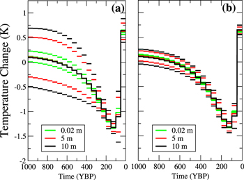
**Figure 4.** GST histories retrieved from inversion of the subsurface temperature anomaly sets in figure 3 for fitting depth ranges of (a) 100 m and (b) 200 m. For each sampling interval, the centre line shows the mean GST history for 1000 anomaly profiles from the Monte Carlo experiment. Outlying curves represent upper and lower bounds for the $95\%$ ( $2\sigma$ ) confidence intervals for each respective sampling interval and colour.
Download figure:
Standard image High-resolution image

**Figure 4.** GST histories retrieved from inversion of the subsurface temperature anomaly sets in figure 3 for fitting depth ranges of (a) 100 m and (b) 200 m. For each sampling interval, the centre line shows the mean GST history for 1000 anomaly profiles from the Monte Carlo experiment. Outlying curves represent upper and lower bounds for the $95\%$ ( $2\sigma$ ) confidence intervals for each respective sampling interval and colour.
Download figure:
Standard image High-resolution image

The Monte Carlo experiments performed above allow a characterization of the variability of the retrieved GST history with respect to sampling interval and fitting depth range. Field data included in the IHFC database, however, rarely contain repeated logs of the same borehole, and never enough to build robust statistics as in the above experiments. To address the estimate of the uncertainty in the IHFC database, we determine the quasi steady-state geothermal field and use the statistical parameters from the linear least-squares fit (mean slope and its $95\%$ confidence intervals) to estimate the range of subsurface temperature anomalies for each BTP. Inversion of the triad of anomalies yields the uncertainties of the GST history retrieved from the inversion. As an example, figure 5(a) shows the GST history (red line) resulting from the SVD inversion for the noise-free subsurface temperature log shown in figure 1(c). The model for the upper boundary condition chosen for the inversion consists of twenty 50 year step changes with an eigenvalue cutoff set at 0.025. Such a limit retains five principal components to reconstruct the GST history (Beltrami et al 2011). Even though the inversion results are for a single noise-free subsurface temperature anomaly, the effects of the loss of resolution due to heat diffusion are readily apparent. In figure 5(b), the upper and lower bounds (blue lines) represent physically derived uncertainties arising from the errors in the determination of the quasi-steady-state geothermal regime, and also from the effects of the surface-energy balance history. These are different from the error bounds provided in previous SVD works (Beltrami et al 1992, Mareschal and Beltrami 1992, Clauser and Mareschal 1995), which represented a measure of the stability of the solution.

**Figure 5.** (a) Recovered GST history for the noise-free synthetic data (red lines). The original upper boundary condition is represented by the solid line. Because of the nature of heat conduction 'sharp edges' are smoothed out and are not recovered. However, the main features of the synthetic GSTH are retrieved. (b) Single BTP example showing the mean GST history (red line) retrieved by inversion. Blue lines represent the upper and lower bounds for the $95\%$ ( $2\sigma$ ) confidence interval obtained from the uncertainty in the semi-equilibrium gradient from the linear fit.
Download figure:
Standard image High-resolution image

The subsurface temperature anomaly inverted for figure 5(b) is for a noise-free case, but the retrieved GST history shows some variability. This arises from the uncertainty in the estimate of the quasi-steady-state geothermal regime induced by the chosen synthetic upper boundary condition, and its propagation into the subsurface. For our particular choice of synthetic GST history at the surface, we would expect that if the generated BTP was sampled more deeply, the effect would be minimized because the fitting-depth interval would remain largely unperturbed by the prescribed surface-energy balance history. We note that in reality, there are a number of processes and characteristics of the lithology in the subsurface, as well as land-surface variability, that induce thermal noise at all depths so that all BTPs contain noise.

3.2. Single BTP example: Minchin Lake, Canada

In order to illustrate the procedure of figure 5 on observed data, we chose a data set often used as a benchmark in Borehole Climatology (Beck et al 1992) and measured continuously by Nielsen and Beck (1989). The set of black points in figure 6(a) represents the data from a Minchin Lake temperature log. For clarity, some points have been removed. The red line represents the semi-equilibrium geothermal gradient estimated from the least-squares fit to the data from the bottom 100 m of the log. The inset shows a detailed view of part of the fitting range with the $95\%$ fitting uncertainties. Figure 6(b) shows the estimated subsurface temperature anomaly derived from the Minchin Lake BTP and a detailed view of the magnitude of the $95\%$ fitting uncertainty for the temperature anomaly.

**Figure 6.** (a) BTP measured at Minchin Lake (black). For clarity, some points have been removed. Steady-state geothermal field was obtained by least squares fit to the bottom 100 m of data in the BTP (red line). Inset: Red line is the best-fit line in the least squares sense. Blue lines denote upper and lower bounds for the $95\%$ ( $2\sigma$ ) confidence interval for the linear fit. (b) Temperature anomaly for Minchin Lake obtained from a linear fit to the bottom 100 m of the BTP. Inset: Details of the upper and lower bounds of the $95\%$ ( $2\sigma$ ) confidence interval for the temperature anomaly.
Download figure:
Standard image High-resolution image

**Figure 6.** (a) BTP measured at Minchin Lake (black). For clarity, some points have been removed. Steady-state geothermal field was obtained by least squares fit to the bottom 100 m of data in the BTP (red line). Inset: Red line is the best-fit line in the least squares sense. Blue lines denote upper and lower bounds for the $95\%$ ( $2\sigma$ ) confidence interval for the linear fit. (b) Temperature anomaly for Minchin Lake obtained from a linear fit to the bottom 100 m of the BTP. Inset: Details of the upper and lower bounds of the $95\%$ ( $2\sigma$ ) confidence interval for the temperature anomaly.
Download figure:
Standard image High-resolution image

To estimate the effects: (a) of a varying depth range on the determination of the quasi-steady-state geothermal gradient and, (b) of the sampling interval of a BTP on the inversion results, we invert the sets of subsurface temperature anomalies for Minchin Lake estimated from a 100 m and a 200 m fitting-depth range. Figures 7(a) and (b) show the inversion results for the Minchin Lake data for the two fitting-depth ranges. The difference of fitting range for this particular example contributes little to the uncertainty envelope for the GST history. This is due to the relatively large depth of the BTP (500 m), and the characteristics of the temporal evolution of the upper boundary condition, whose changes have decayed significantly at the depth of both fitting ranges (Beltrami et al 2011, 2014a).

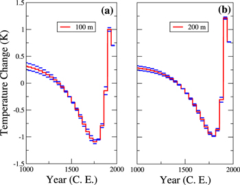
**Figure 7.** A set of GST histories estimated for Minchin Lake (black lines) for (a) 100 m range and (b) 200 m range used to estimate the quasi-steady state equilibrium profile (reference). The blue lines in each panel indicate the uncertainty envelope estimated from the uncertainty of the linear fit obtained for the geothermal gradient and the long-term surface temperature in each example.
Download figure:
Standard image High-resolution image

This situation would be different for shallower BTPs, where the fitting range may include a significant part of the subsurface climatic temperature anomaly. In general, larger fitting-depth ranges provide more stable estimates of the quasi-stead-state in the subsurface, but they remove valuable climatic information, particularly when dealing with shallow boreholes.

Figures 8(a)–(c), show the GST histories for Minchin Lake for a fitting-depth range of 100 m, with sampling intervals of 0.02 m, 5 m, and 10 m. We note that the BTPs were sampled before carrying out a least-squares fit of the semi-equilibrium geothermal gradient. As expected, the increased sampling interval significantly reduces the maximum uncertainties by about an order of magnitude when the sampling interval increases from 10 m to 0.02 m. The sampling interval of the majority of the BTPs in the IHFC database is 10 ${\rm m}$ .

**Figure 8.** A set of GST histories estimated for Minchin Lake (black lines) for three sampling intervals: (a) 10 m, (b) 5 m and (c) 0.02 m. The deepest 100 m of the profiles were used to estimate the quasi-steady-state equilibrium profile (reference) in each case. The blue lines in each panel indicate the uncertainty envelope estimated from the uncertainty of the linear fit obtained for the geothermal gradient and the long-term surface temperature in each example.
Download figure:
Standard image High-resolution image

As the subsurface energy budget plays a role in ascertaining the overall energy budget of the climate system (see figure 1 in box 3 Rhein et al 2013), we examine the uncertainties related to the estimate of continental heat. The subsurface heat content, Q_s, is given by the integral of the temperature anomalies over a given depth range; i.e.,

$\begin{eqnarray}&&{{{\rm Q}}_{{\rm s}}}=\rho {\rm C}\int _{{{Z}_{i}}}^{{{Z}_{f}}}\Delta {\rm T}(z){\rm d}z,\end{eqnarray} \tag{ 2 }$

where $\rho$ and ${\rm C}$ are the mass density and volumetric heat capacity, respectively, and are dependent on the thermal properties of the subsurface rocks; Z_f and Z_i represent the initial and final depth of the depth range under consideration. $\Delta {\rm T}(z)$ is the subsurface temperature anomaly as a function of depth. Figure 9 shows the subsurface heat storage as a function of depth, Q_s, for the Minchin Lake site. The curve shows Q_s from the surface to the indicated depth. There is clear indication that at this site, the heat content is largest near the surface for about 100 m, indicating recent warming, and then decreases continuously until 300 m, indicating the recovery from a previous colder period. Below this depth, Q_s appears to be constant. This is the expected result from a BTP that has been under the influence of the cold Little Ice Age period previously reported from BTP data in Canada (e.g. Beltrami et al 1992, Mareschal and Beltrami 1992, Shen and Beck 1992).

**Figure 9.** Total heat content as a function of depth for Minchin Lake. The calculation is the integral of the temperature anomaly from 20 m down to the given depth. Red line represents the heat content calculated from the mean temperature anomaly, while the blue lines represent the maximum and minimum values of the energy storage.
Download figure:
Standard image High-resolution image

3.3. Northern Hemisphere dataset

The IHFC dataset for borehole climatology contains 611 temperature-depth profiles for the Northern Hemisphere. Because the measurements, with a few exceptions, were carried out in boreholes of opportunity, the data have an uneven spatial distribution and their depth ranges vary between the minimum depth for the database inclusion, 200 m, and about 600 m. As shown in figure 10, most of the BTPs are shallow ( 200 m) except for the regions over northern Canada and central Europe where boreholes with depths ranging up to 600 m or greater are found. Figure 11(a) shows the spatial distribution of the long-term surface temperatures ( ${{T}_{0}}$ in equation (1)) calculated by performing a linear least-square fit over the bottom-most 100 m of each of the BTPs in the dataset. Because the atmosphere is coupled to the ground surface, ${{T}_{0}}$ increases with decreasing latitudes as expected. Figure 11(b) shows the 95% confidence ranges for ${{T}_{0}}$ . As evident from this figure, the error-bounds are small for most of the locations and range to a maximum of $\pm 0.5{\rm K}$ for some regions where the BTPs are shallow. Similarly, figure 11(c) shows the spatial distribution of the estimated magnitude of the semi-equilibrium heat-flow density, ${{q}_{0}}$ , from the Earthʼs interior for the region. Because there are few measurements of the thermal properties of the subsurface, the estimates of ${{q}_{0}}$ are based on an assumed constant thermal conductivity of $3.0\;{\rm W}{{{\rm K}}^{-1}}\;{{{\rm m}}^{-1}}$ (Beltrami et al 2006, MacDougall et al 2008, 2010). Figure 11(d) shows the 95% confidence levels for ${{q}_{0}}$ . The uncertainties for ${{q}_{0}}$ can be as high as 20% for some regions, such as parts of western North America.

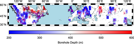
**Figure 10.** Spatial distribution of borehole temperature profiles (dots) for the Northern Hemisphere from the IHFC database. Sites are unevenly distributed and have a range of depths because measurements are conducted in boreholes of opportunity. Borehole depths are indicated in the legend bar.
Download figure:
Standard image High-resolution image

**Figure 11.** (a) Spatial distribution of the long-term surface temperature, ${{T}_{0}}$ , estimated from the semi-equilibrium steady-state temperature versus depth profiles. (b) 95% confidence ranges for (a). (c) Spatial distribution of the semi-equilibrium heat-flow density, ${{q}_{0}}$ , from the interior of the Earth, i.e., the long-term lower boundary condition for an assumed homogeneous subsurface with thermal conductivity set at λ = 3 Wm⁻¹K⁻¹, (d) 95% confidence ranges for ${{q}_{0}}$ for (c).
Download figure:
Standard image High-resolution image

**Figure 11.** (a) Spatial distribution of the long-term surface temperature, ${{T}_{0}}$ , estimated from the semi-equilibrium steady-state temperature versus depth profiles. (b) 95% confidence ranges for (a). (c) Spatial distribution of the semi-equilibrium heat-flow density, ${{q}_{0}}$ , from the interior of the Earth, i.e., the long-term lower boundary condition for an assumed homogeneous subsurface with thermal conductivity set at λ = 3 Wm⁻¹K⁻¹, (d) 95% confidence ranges for ${{q}_{0}}$ for (c).
Download figure:
Standard image High-resolution image

The effects of the uncertainties of ${{T}_{0}}$ and ${{q}_{0}}$ on the determination of GST histories are illustrated in figure 12(a), which shows the spatial distribution of the results of the SVD inversion of all 611 BTPs for the last 50 years of the 20th century. Figure 12(b) shows the corresponding 95% confidence bounds. The largest uncertainties for this period ( $\pm 0.5\;{\rm K}$ ) correspond to areas with the largest ${{T}_{0}}$ uncertainty (figure 11(b)).

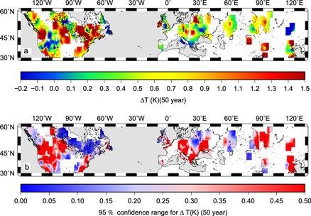
**Figure 12.** (a) Spatial distribution of the first 50 years, (1950–2000 of the Common Era) ( $\Delta {{T}_{50}}$ ), of the GST histories recovered from inversion. The figures are constructed from 611 BTPs in the Northern Hemisphere between ${{30}^{o}}\;{\rm N}$ and ${{60}^{o}}\;{\rm N}$ . The same number of principal components were included in the reconstruction of each GST history. (b) 95% confidence ranges for $\Delta {{T}_{50}}$ derived from the determination of the quasi-steady-state profile uncertainties.
Download figure:
Standard image High-resolution image

A similar situation is expected for the evaluation of the subsurface heat content, Q_s, from this dataset. However, as Q_s is proportional to the depth of the temperature anomaly in the subsurface (equation (2)), then theoretically, two BTPs subject to the same climatic history would yield different values of Q_s if sampled to different depths. Thus, it is necessary to use only the estimates of this quantity within the same depth range. Figure 13(a) shows the spatial distribution of the subsurface heat content over a truncation depth of 200 m. Figure 13(b) displays the corresponding 95% confidence range. These uncertainties on Q_s are large because the error on ${{T}_{0}}$ and ${{q}_{0}}$ map onto the complete profile of the subsurface temperature anomaly such that the uncertainties at all depths are cumulative over a volume.

**Figure 13.** (a) Spatial distribution of the subsurface heat content. Because subsurface heat content is proportional to the integral of the temperature anomaly underground, it depends on BTP depth. Thus the estimates shown here are based on 611 boreholes truncated at a depth of 200 m. (b) 95% confidence ranges derived from the determination of the quasi-steady state profile uncertainties. The uncertainties are largest at the location of shallower BTP.
Download figure:
Standard image High-resolution image

There is a clear correlation between the areas where the uncertainties are large for Q_s, and those areas in figure 10 that contain the shallower BTPs. In northern Canada, where the majority of deep boreholes are located, uncertainties for ${{T}_{0}}$ and ${{q}_{0}}$ , and therefore for Q_s and the GST histories, are lower. This is also the case in parts of eastern Europe.

4. Conclusions

We have examined the effects of uncertainties in the determination of the quasi steady-state thermal regime of the subsurface and provided error bounds for the estimated GST history and Q_s for the IHFC dataset for the Northern Hemisphere. Our uncertainties in the estimates of the quasi-steady-state geothermal regime are obtained from the data, and they map onto the model chosen for the GST history inversion. We find that choosing a large depth range for estimating the quasi-steady-state geothermal gradient provides a statistically stable value, but it also removes valuable climatic information from the data, particularly when analyzing shallow boreholes. On the other hand, high data-sampling intervals also provide a statistically stable estimate of the quasi-steady-state geothermal gradient, without removing valuable climatic information. Estimating the magnitude of Q_s does not require inversion, that is the assumption and evaluation of a model for the time evolution of the upper boundary condition. However, the uncertainties in the estimate of the quasi steady-state geothermal regime also map onto the estimate of subsurface heat content, Q_s. Because Q_s is proportional to the integral of the subsurface temperature anomaly (equation (4)), uncertainties in Q_s can be large. Thus, for estimating GST histories and Q_s we strongly recommend continuous logging of temperature-versus-depth profiles to reduce uncertainties. We also note that the estimated values of ${{T}_{0}}$ and ${{Q}_{0}}$ could serve as initial- and bottom-boundary conditions for land-surface model components that seek to characterize near-surface, energy-dependent processes. Finally, the uncertainties that we have quantified in this study provide a better constraint on the range of possible GST histories and Q_s values over the last millennium. These uncertainties should be a standard element of future reconstructions from borehole paleoclimate data in order to better characterize the true range of uncertainties inherent in such efforts.

Acknowledgments

H Beltrami is supported by grants from the Natural Sciences and Engineering Research Council of Canada Discovery Grant program (NSERC-DG) and the Atlantic Innovation Fund (AIF-ACOA). We also thank ACEnet for computational resources, and the Lamont-Doherty Earth Observatory contribution number 7855. The IHFC dataset for Borehole Climatology is available at http://ncdc.noaa.gov/data-access/paleoclimatology-data/datasets/borehole.

Ground surface temperature and continental heat gain: uncertainties from underground

Article metrics

Submit

Author e-mails

Author affiliations

Dates

Peer review information

Abstract

1. Introduction

2. Theoretical background

3. Analysis, results and discussion

3.1. Synthetic data experiments

3.2. Single BTP example: Minchin Lake, Canada

3.3. Northern Hemisphere dataset

4. Conclusions

Acknowledgments

Ground surface temperature and continental heat gain: uncertainties from underground

Article metrics

Submit

Share this article

Author e-mails

Author affiliations

Dates

Peer review information

Abstract

1. Introduction

2. Theoretical background

3. Analysis, results and discussion

3.1. Synthetic data experiments

3.2. Single BTP example: Minchin Lake, Canada

3.3. Northern Hemisphere dataset

4. Conclusions

Acknowledgments