


Abstract
Grain boundaries and defect lines in graphene are intensively studied for their novel electronic and magnetic properties. However, there is not a complete comprehension of the appearance of localized states along these defects. Graphene grain boundaries are herein seen as the outcome of matching two semi-infinite graphene sheets with different edges. We classify the energy spectra of grain boundaries into three different types, directly related to the combination of the four basic classes of spectra of graphene edges. From the specific geometry of the grains, we are able to obtain the band structure and the number of localized states close to the Fermi energy. This provides a new understanding of states localized at grain boundaries, showing that they are derived from the edge states of graphene. Such knowledge is crucial for the ultimate tailoring of electronic and optoelectronic applications.
Export citation and abstract BibTeX RIS

Content from this work may be used under the terms of the Creative Commons Attribution 3.0 licence. Any further distribution of this work must maintain attribution to the author(s) and the title of the work, journal citation and DOI.
1. Introduction
Experimentally grown graphene presents grain boundaries which have been clearly observed by several techniques, for example, high-resolution transmission electron microscopy [1, 2]. Grain boundaries have been measured to affect electronic transport in graphene [3–5] and are the subject of ongoing research [2, 6–8]. As a matter of fact, grain boundaries present localized states, which have been proven to be crucial, with distinct electronic [9, 10], magnetic [11] and mechanical [12] properties that depend on the atomic line junctions. These localized states also allow for the decoration of line defects with adsorbates [6, 13], which opens a novel route for nanosensor applications. As the electronic and optoelectronic properties of graphene are modified by the localized states at the boundaries [14], the ultimate control of graphene-based products and devices requires the tailoring and engineering of grain boundaries.
Electronic transport through extended defect lines has been previously studied and explained in terms of folding the band structure of graphene [15–17]. However, the relation between the geometry of grain boundaries and the induced electronic localized states has not been clarified yet. Here we treat the defect lines as the outcome of matching two graphene sheets with different edges, which produces localized states. Recently, general rules to predict the existence of edge states and zero-energy flat bands in graphene nanoribbons and graphene edges of arbitrary shape have been given [18]. Previous works on junctions between armchair and zigzag carbon nanotubes have proved that interface states, customarily attributed to the presence of topological defects at interfaces, are actually related to zigzag edge states, like those of truncated graphene [19]. Additionally, localization at chains of grain boundaries with octagonal defects has been already understood as a consequence of the zigzag nature of the graphene edges forming the defect lines [20]. We are now bringing into contact these ideas about localized states in graphene edges to give a more comprehensive explanation of states appearing in extended defect lines in graphene.
In this paper, we focus on how grain boundaries modify the electronic properties of intrinsic graphene, i.e., with zero carrier density. Our main results are the following.
- (i)We present a theory of localized states around the Fermi energy (EF) in intrinsic graphene due to the grain boundaries built of pentagon/heptagon (5–7) defects, which are equivalent to defect lines at junctions between two graphene sheets.
- (ii)Depending on the geometries of the joined edges we find three distinct and well defined electronic behaviors.
- (iii)Furthermore, we are able to give the number of bands near EF for any periodic grain boundary.
Our approach offers a new insight on the origin of these localized states, and allows for the prediction of their electronic characteristics without performing numerical calculations.
2. Theory
In this section we explain how to find the near-EF energy spectra of grain boundaries, based on the detailed structure of the two constituent graphene edges, considering semi-infinite graphene sheets with different edges, joined to make a grain boundary. Indeed, for infinite systems without periodicity in one direction, the tight-binding approximation combined with a Green function matching technique emerges naturally as a method of choice. We further corroborate our results by nearest-neighbor, π-orbital tight-binding calculations for several instances. We use the same hopping ( eV) for all bonds. A slight variation of this value at the grain boundaries modifies a little the numerical result, but does not affect the number of final edge states. In fact, grain boundaries undergo structural relaxations [21] that amount to changes in the hopping parameters in our model; however, it has been previously shown that tight-binding band structures with a fixed hopping in carbon nanostructures have a good agreement with DFT calculations once atoms were fully relaxed around the Fermi energy [22]. The density of states (DOS) at the junction is obtained by means of the Green function matching technique [23]. Grain boundaries composed of topological 5–7 defects are herein viewed as the result of joining two graphene edges with different orientations. Recall that all graphene edges—with the exception of the pure armchair case—have flat edge-localized bands at EF, which for intrinsic graphene is at zero energy within our model. We aim at understanding the energy spectra of grain boundaries or graphene interfaces from the hybridization and splitting of graphene edge bands. We concentrate on straight boundaries built up of two periodic minimal edges [24], i.e., those with a minimum number of edge nodes with coordination number 2 per translation period. Other types of edges can be constructed by adding extra nodes to minimal edges and their properties can also be studied along the lines presented below.
Periodic minimal edges are characterized by the edge translation vector  , where
  ,
,  are two graphene lattice vectors forming a
  angle. The edge vector
  can be decomposed in a zigzag and an armchair part,
  , which are the projections of
  along the zigzag (
 ) and the armchair (
 ) direction, respectively. It was recently shown [18] that the low-energy spectrum of a minimal graphene edge, i.e., the number and degeneracy of flat bands near EF, is uniquely determined by its zigzag component
  . The band structure around EF of a general (n, m) edge can be obtained by folding
  times the spectrum of a pure (1,0) zigzag edge [18]. This gives not only the number of zero-energy bands, but also the position of the Dirac point after folding and therefore the shape of the band continua. Setting

where  and
and  makes possible a simple identification of the different classes of spectra for edges with
  . The pure armchair edge would correspond to the case I = 0 and M = 0. The four types of spectra are shown in figure 1. The number I defines the type of edge as to its spectrum, and the number of edge bands equals M or
  depending on the type of edge and the value of the wavevector k. The pure armchair edge, without edge bands, corresponds to I = 0 and M = 0. Note that the E = 0 bands are mostly localized at one sublattice, and those corresponding to
  in the unfolded
  zigzag edge are almost exclusively localized6
at the edge zigzag-like nodes.
zigzag edge are almost exclusively localized6
at the edge zigzag-like nodes.

Figure 1. The four different classes of band edge spectra for minimal graphene edges. The value of I identifies the type of spectrum, and M or  counts the number of edge bands. Gray areas schematically represent the band continua.
Download figure:
Standard image High-resolution imageIn general, the connection of two different minimal edges produces topological defects at the interface between them. In order to achieve grain boundaries composed of hexagons, pentagons and heptagons with coordination number 3, which are more energetically favorable, the two edges (n, m) and  should verify
  , where all the nodes have coordination 3. For such a grain boundary

where q is the number of 5–7 defects in the interface unit cell. Note that if  is not equal to
  , the joined edges have different number of edge nodes per translation period, so either some of them have coordination number less than 3 or other topological defects instead of pentagons and heptagons are needed. Such junctions can be studied along the lines presented in this manuscript, but formed from non-minimal edges, as discussed in [18].
When two edges are connected and the grain boundary is formed, their matching edge-localized states hybridize and split, due to the formation of new bonds. The splitting is especially strong for the states corresponding to the unfolded  case, since the corresponding wavefunctions are localized mainly at the outermost edge zigzag nodes; the split bands may reach the energy continua.
As a rule of thumb, the spectrum of a grain boundary is obtained by overlapping the spectra of the two edges. States with the same wavevectors coming from different edges hybridize and split, and the remaining unpaired bands constitute the interface band structure. These remaining bands stem from only one edge. Due to the presence of topological defects, interface states are not necessarily at EF = 0, but are displaced due to the breaking of electron-hole symmetry. They can also split due to the perturbing presence of the other edge, but this splitting is weaker, so these bands remain in the gap, closer to EF.
We first consider one particular case to illustrate this rule. The geometry of the junction (5,0)/(4,1) is depicted in figure 2(a). The (5,0) edge has I = 2 and M = 1, while the (4,1) edge decomposes as (3,0) + (1,1), so it has  ,
,  . Their schematic spectra are shown in figures 2(b) and (c), respectively. The (5,0) edge has one band in the entire Brillouin zone (BZ) and another band spanning from k = 0 to the Dirac point at
  . The (4,1) edge has one band throughout the BZ and its Dirac point is at k = 0. This latter (4,1) edge band hybridizes with its counterpart from the (5,0) edge, leaving one interface band which extends between the two Dirac points, from k = 0 to
  . This is depicted in figure 2(d). For comparison, we plot in figure 2(e) the DOS projected at the grain boundary as a function of the energy and wavevector parallel to the junction, calculated within the tight-binding approximation. Both the interface band and the continua of the two bulk media can be clearly distinguished in this projected DOS, in complete agreement with the outcome of our rule, shown in figure 2(d).
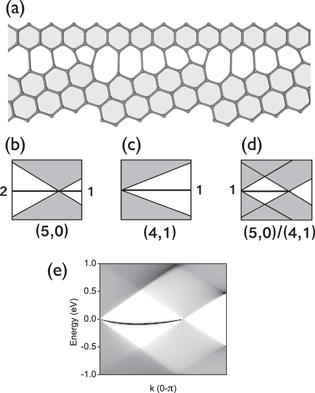
Figure 2. (a) Geometry of a (5,0)/(4,1) grain boundary. (b), (c) Schematic energy spectra of the (5,0) and (4,1) edges, respectively; (d) schematic spectrum of the (5,0)/(4,1) boundary, in good agreement with (e) the projected DOS at the (5,0)/(4,1) boundary. Darker color indicates a larger DOS value.
Download figure:
Standard image High-resolution imageFor a general graphene grain boundary composed of two minimal edges, the combination of the four possible band structures shown in figure 1 gives rise to ten different schematic grain boundary spectra, presented in figure 3. According to the number and position of the Dirac points and the corresponding continua, there are three kinds of spectra: (i) one Dirac point at  ; (ii) one Dirac point at k = 0; and (iii) two Dirac points at k = 0 and
  . Case (i) occurs when the spectral types of joined edges are
  . The degeneracy of grain boundary bands with the energies close to EF, depends on the particular combination of I and
  , being their number either
  ,
,  , or
, or  . For
. For  they are exactly
  and their number is the same at both sides of the Dirac point. For
  the number of bands at both sides of the Dirac point differs by two. In case (ii) there is only one Dirac point at k = 0 and there are
  interface bands. This situation arises when joining edges with
  . It also includes the junction of an I = 3 edge with an armchair edge
  , for which the number of interface bands is
  . Case (iii) with two distinct Dirac points, presents a different number of interface bands at each side of the Dirac point at
  , but the difference is just one band. Figure 3 at the bottom row also enumerates the case of interfaces between an armchair edge without flat bands and any other kind of edge, which sets the number of final bands for the boundary. Thus, the knowledge of I and
  for two particular edges fixes the kind of spectrum; giving the values of M,
  for the constituent edges completely determines the number of bands and their wavevector range at the grain boundary.
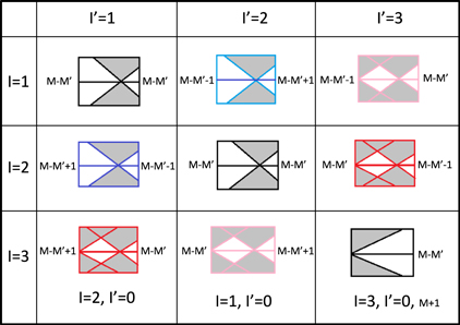
Figure 3. Summary of the possible grain boundary band structures as a function of the edge types I,  . The number of edge bands, related to
  , is given for each case close to EF. Grain boundaries built by the junction of an armchair edge
  with any other type can be assimilated to the last row of the table. For this latter cases only the number of bands near EF for I = 3,
  is different from those close to the schematic bands, (
 instead of
  ), and explicitly indicated in the corresponding cell of the table. The different number of states between the k points k = 0 and
  are denoted by different colors: 2 with dark blue, 1 with red, 0 with black, −1 with pink, and −2 with light blue.
Download figure:
Standard image High-resolution imageIn fact, we also derive a formula for the number of the interface bands, which is basically given by  plus/minus one band. We already discussed that for a junction involving an edge with indices
  , the other edge should have indices (n, m). From equation (1), their corresponding types are given by

so it follows that

This formula implies that even though there is a relation between the number of topological defects q and the number of grain boundary bands, related to  , the classes of edges
  involved in the interface are determinant for the outcome. In particular, different boundaries with the same number of topological defects may have different interface bands. As an example, the (4,0)/(3,1) and the (3,1)/(2,2) boundaries both have one 5–7 defect (q = 1), but their spectra are different: the (4,0)/(3,1) case has I = 1,
  and M = 1,
  , with two edge bands from
  to
to  (see figure 3), while the (3,1)/(2,2) grain boundary has
  , I = 0 and
  , which results in one edge band from k = 0 to
  .
.
It is noteworthy that q is not a free variable in equation (3), but for a given pair of I,  is determined by the requirement that
  has an integer value.
3. Further examples
In the previous section we described in detail one interface having the energy spectrum with two Dirac points. Here we present results of calculations for two more instances representing the other two possible spectra, namely, one Dirac point at k = 0 and one Dirac point at  .
.
3.1. Dirac points at k = 0: (10,1)/(7,4)
When  the spectra of the constituent edges have the Dirac point at k = 0. From equation (3) it is clear that the number of defects q has to be a multiple of 3. One of the possible examples with the minimum q = 3 is the junction between the (10,1) and (7,4) edges. The (10,1) edge has three zero-energy edge bands in the entire BZ, whereas the zero-energy spectrum of the (7,4) edge is the same as of the (3,0) edge, i.e., a single E = 0 band in the BZ. This band strongly mixes with one of (10,1) edge bands, so they split, merging in the positive and negative energy band continua. Two bands are left, stemming from the (10,1) edge.
The unit cell of the (10,1) edge is almost entirely composed of zigzag nodes, with one armchair step. The unit cell of (7,4) edge has three zigzag nodes and four armchair steps that can be distributed in different ways, as shown in figure 4(a) and (b). Therefore, we can construct two different junctions between (10,1) and (7,4) edges, which distinct distributions of 5–7 topological defects along its length. One junction has the sequence 6-5-7-6-5-7-6-6-6-5-7, and the other is 6-6-5-7-5-7-6-6-6-5-7. These two different positions of three 5–7 defects at the interface produce differences in the interaction and splitting of the remaining bands of the (10,1) edge, so they yield different spectra. They are shown in figure 4(c) and (d). Although the dispersion of the bands in these two cases is clearly distinct, the number of edge states in the energy gap, near EF, is the same as predicted by our hybridization rule.

Figure 4. (a), (b) Two possible geometries of the (7,4) edge; the zigzag edge nodes are marked by circles. (c), (d) The projected DOS for two different (10,1)/(7,4) boundaries obtained from the two edges depicted in (a) and (b). Red arrows indicate the grain boundary states.
Download figure:
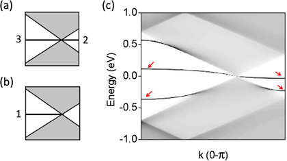
Standard image High-resolution image3.2. Dirac points at  : (8,0)/(5,3)

If the edges composing the boundary have  , the spectrum of the resulting interface has the Dirac points at
  . To illustrate these cases, we have chosen a junction between (8,0) and (5,3) graphene edges. Before the edges are connected, the (8,0) edge has two E = 0 bands in the entire BZ and one band spanning between k = 0 and the Dirac point at
  , as shown in figure 5(a). The (5,3) edge has a (2,0) zigzag component, thus it has one E = 0 band between k = 0 and the Dirac point, see figure 5(b). This band strongly interacts with its counterpart of the (8,0) edge; they hybridize and split by more than 1.3 eV at k = 0. The projected DOS is presented in figure 5(c). One of the split bands enters the negative energy band continuum and mixes with the continuum states, so it no longer yields a peak in the calculated DOS. The other one almost reaches the positive continuum, for k = 0 its energy equals 0.55 eV, although it is still appreciable in the figure. The two remaining boundary bands—which originate from the (8,0) edge—also split, but they are still present in the gaps on both sides of the Dirac point. Their splitting at the right side of the BZ is weaker than the splitting at the BZ center, since they are closer to the Dirac point, where they are pinned. The structure and number of localized bands around Fermi energy calculated in figure 5 coincide with those schematically shown in figure 3.
Figure 5. (a), (b) Schematic spectra for (8,0) ( ) and (5,3) (
 ) edges, respectively. (c) Projected DOS at the grain boundary (8, 0)/(5,3). Red arrows indicate the grain boundary states.
Download figure:
Standard image High-resolution image
4. Summary and conclusions
We have studied grain boundaries in graphene built of pentagons, heptagons and hexagons. Such defect lines can be seen as junctions between two graphene edges. We have shown that energy states localized at grain boundaries have their origin in the states localized at the graphene edges with energies at the Fermi level. We have classified all the possible energy spectra at the periodic grain boundaries in graphene, and reduced them to a few types only. We have found a simple formula for determining the number of interface bands with energies in the gap and close to EF. When two edges are connected, the edge-localized states interact and mix. The states which are localized at different edges strongly hybridize and thus markedly split, usually reaching the energy band continua. States localized at one edge are affected by the presence of the neighboring edge, their energies are displaced slightly from EF. In the case of degeneracy they also split, but the splitting is weaker, leaving such states still close to the Fermi level, although the value of splitting depends on the particular structure of the junction.
The number of localized bands at the grain boundary is determined by the types of the energy spectra of the joined edges, not just by the number of 5–7 defects at the interface. In fact, junctions having the same number of defects at the interface unit cell may have a different number of interface-localized bands.
Our procedure allows for an easy prediction of the number of interface localized states with energies close to the Fermi level for any periodic grain boundary in graphene. Although we have focused on minimal edges, our approach can be also applied to non-minimal ones. As detailed in [18], bands for general edges can be understood by applying hybridization rules to the atoms added to obtain the non-minimal edge. From the resulting edge band structures, the final grain boundary spectrum with their localized bands can be derived as explained herein. Although this is beyond the scope of the present work, we have checked that our procedure can be extended to the matching of non-minimal borders giving rise to more complex line defects [25, 26]. Likewise, the same approach can be used to determine the existence of states localized at finite, non-periodic grain boundaries in graphene, since in these cases the BZ reduces to one point.
Our classification of the interface localized states brings a basic understanding on grain boundaries in graphene to both experimentalists and theoreticians. This method to find localized bands around the Fermi energy is important for defect engineering towards practical electronic and optoelectronic [14] applications based on graphene and carbon nanotubes, which strongly depend on the spectrum near the Fermi energy.
Acknowledgements
This work was supported by the Polish National Science Center (grant DEC-2011/03/B/ST3/00091), the Basque Government through the NANOMATERIALS project (grant IE05-151) under the ETORTEK Program (iNanogune), the Spanish Ministerio de Ciencia y Tecnología (grants FIS2010-21282-C02-02, FIS2012-33521 and MONACEM projects), and the University of the Basque Country (grant no. IT-366-07). We acknowledge the Nicolaus Copernicus University in Toruń (AA and LC) and the DIPC (WJ, HS and LC) for their generous hospitality.
Footnotes
- 6
Exclusively—for pure zigzag edges only.