


Abstract
We present a new photometric method by which improved high-precision reddenings and true distance moduli can be determined to individual Galactic Cepheids once distance measurements are available. We illustrate that the relative positioning of stars in the Cepheid period–luminosity (PL) relation (Leavitt law) is preserved as a function of wavelength. This information then provides a powerful constraint for determining reddenings to individual Cepheids, as well as their distances. As a first step, we apply this method to the 59 Cepheids in the compilation of Fouqué et al. Updated reddenings, distance moduli (or parallaxes), and absolute magnitudes in seven (optical through near-infrared) bands are given. From these intrinsic quantities, multiwavelength PL and color–color relations are derived. We find that the V-band period–luminosity–color relation has an rms scatter of only 0.06 mag, so that individual Cepheid distances can be measured to 3%, compared with dispersions of 6 to 13% for the one-parameter K through B PL relations, respectively. This method will be especially useful in conjunction with the new accurate parallax sample upcoming from Gaia.
Export citation and abstract BibTeX RIS
1. Introduction
In recent decades, the calibration of the Cepheid extragalactic distance scale has relied, in large measure, on observations of Cepheids in nearby galaxies (e.g., the LMC, M31, and NGC 4258; noting, for example, Freedman et al. 2001, 2012; Riess et al. 2016, and references therein). The Milky Way has historically been bypassed for the simple reason that very few long-period Cepheids are sufficiently close to measure their distances accurately, and none have been found in open clusters, near or far; therefore measurement of the slope of the period–luminosity (PL) relation (or Leavitt law) has been more robustly carried out using external galaxies where large, statistically complete samples of Cepheids at all periods are available. Progress on measurement of parallaxes for MW Cepheids has come from HST with the measurement of 10 Cepheids by Benedict et al. (2007) and two additional stars (both of which are long-period Cepheids) measured by Riess et al. (2014) and Casertano et al. (2016). Still, the sample of Benedict contains only a single Cepheid, l Car, with a period longer than 10 days. In contrast, most of the extragalactic searches have targeted Cepheids with periods mostly greater than 10 days.
Measurement of parallaxes, however, is only the first step in the PL calibration. Not only parallaxes but also wavelength-dependent corrections for interstellar extinction are required to obtain absolute magnitudes. Cepheids are young and rare, F and G-type supergiants. As such, they are sparsely distributed throughout the galaxy, and their apparent magnitudes are generally reddened and attenuated by intervening interstellar dust of varying amounts. Each Cepheid has a unique line of sight and reddening. These effects must be corrected for at each observed wavelength before intrinsic relations can be derived: both distances and extinctions must individually be derived independently for each star.
Many methods have been used for determining the total line-of-sight reddenings to individual Cepheids both in the Milky Way and in the nearest galaxies. In general, the quoted uncertainties in the reddenings range from ±0.03 to 0.05 mag in E(B − V). For our purposes in this study, we have adopted the Fouqué et al. (2007) sample of Galactic Cepheids, and we will use their absolute magnitudes and mean reddenings simply to illustrate our methodology designed to refine and produce high-precision reddenings. Making use of a reddening-independent magnitude to establish the relative positioning of individual stars within the PL relation, we use multiwavelength data to constrain the reddening estimates to individual Cepheids and to refine their distances. Initially, we began this investigation with the goal of improving reddenings to Cepheids. It later became clear that not only the reddenings could be improved, but the individual distance moduli themselves could be self-consistently updated as well.
2. The Sample
We have used a published compilation of absolute magnitudes measured in seven bands, based on distances and reddenings independently determined for 59 Galactic Cepheids (Fouqué et al. 2007), with overtone and suspected overtone pulsators omitted. Where available, HST parallaxes have been adopted for these stars, followed by Infrared Surface Brightness (IRSB) determinations and then Interferometric Baade-Wesselink applications and, finally, revised Hipparcos parallaxes. A comprehensive discussion of these methods and all relevant references are given in Fouqué et al. Other data sets could have been considered, such as the more recent IRSB distances found in Storm et al. (2011) or those published by Groenewegen (2013); however, the purpose of this paper is not to give a final answer, but rather to introduce and test a technique in anticipation of the release of astrometric high-precision parallaxes from the Gaia mission. For this same reason there is no critiquing of the methods or implicit calibrations used in Fouqué et al. (2007) because our goal is to introduce and explain a new methodology, applied to an exemplary data set.
We start with a quick review of the basic attributes of the various PL relations relevant to the corrections detailed in the main body of this paper.
Figure 1 shows an expanded view of the B-band PL relation for the Milky Way Cepheids contained in Table 7 of Fouqué et al. (2007) and repeated for completeness and convenience of comparison in Table 1 of the present paper. We identify each of the stars for which there are HST parallaxes, using larger symbols. It can be seen immediately that this high-precision subset of the total sample does fairly outline the total width of the PL relation ( being on the 2σ, bright (blue) edge of the instability strip and
  falling on the faint (red) edge). These stars also span almost the entire range of periods encompassed by the parent sample, falling short by about 0.1 in log P at the bright end. These same variables will be tracked into the revised B-band PL relation (Figure 15), to be presented later in this paper.

Figure 1. Uncorrected intrinsic PL Relation for 59 Galactic Cepheids in the B band, as published by Fouqué et al. (2007). Cepheids with HST parallaxes from Benedict et al. (2007) are marked as larger doubly circled circles and are individually identified and labelled. It is noteworthy that this HST-selected subset of the total sample of Galactic Cepheids is clearly representative of the larger sample, given that they cover the full width of the instability strip, especially well in the short-period range. In this rendition,  falls on the faint/red edge of the instability strip at the long-period end of this PL relation. It would then be expected to flatten the slope of any PL relation (as is noted in the text), relying on just these 10 Cepheids.
Download figure:
Standard image High-resolution imageTable 1. Properties of 59 Galactic Cepheids
| Cepheid | log(P) | E(B − V) |

|
π (
|
MB | MV | MR | MI | MJ | MH | MK |
|---|---|---|---|---|---|---|---|---|---|---|---|
| days | mag | mag | mas | mag | mag | mag | mag | mag | mag | mag | |
| RT Aur | 0.571489 | 0.059 | 8.099 | 2.400 (0.19) | −2.31 | −2.84 | −3.20 | −3.40 | −3.94 | −4.15 | −4.24 |
| 0.202 | 8.169 | 2.324 (0.40) | −1.64 | −2.31 | −2.79 | −3.11 | −3.74 | −3.99 | −4.12 | ||
| QZ Nor | 0.578244 | 0.253 | 10.512 | 0.790 (0.10) | −1.83 | −2.47 | −2.85 | −3.15 | −3.67 | −3.91 | −4.01 |
| 0.184 | 10.258 | 0.888 (0.98) | −2.37 | −2.94 | −3.27 | −3.51 | −3.99 | −4.21 | −4.29 | ||
| SU Cyg | 0.584952 | 0.098 | 9.622 | 1.190 (0.05) | −2.61 | −3.08 | −3.38 | −3.63 | −4.08 | −4.28 | −4.36 |
| 0.163 | 9.625 | 1.188 (0.03) | −2.34 | −2.87 | −3.22 | −3.53 | −4.02 | −4.24 | −4.33 | ||
| Y Lac | 0.635863 | 0.207 | 11.783 | 0.440 (0.02) | −2.79 | −3.31 | −3.65 | −3.90 | −4.33 | −4.58 | −4.66 |
| 0.263 | 11.979 | 0.402 (1.90) | −2.36 | −2.94 | −3.32 | −3.62 | −4.08 | −4.35 | −4.44 | ||
| T Vul | 0.646934 | 0.064 | 8.606 | 1.900 (0.23) | −2.48 | −3.06 | −3.41 | −3.66 | −4.12 | −4.36 | −4.45 |
| 0.170 | 8.654 | 1.858 (0.18) | −1.99 | −2.67 | −3.11 | −3.45 | −3.98 | −4.25 | −4.36 | ||
| FF Aql | 0.650397 | 0.196 | 7.756 | 2.810 (0.18) | −2.46 | −3.02 | −3.35 | −3.64 | −4.09 | −4.29 | −4.37 |
| 0.183 | 7.606 | 3.011 (1.12) | −2.66 | −3.21 | −3.53 | −3.81 | −4.25 | −4.45 | −4.52 | ||
| T Vel | 0.666501 | 0.289 | 10.022 | 0.990 (0.01) | −2.28 | −2.93 | −3.32 | −3.64 | −4.13 | −4.41 | −4.51 |
| 0.189 | 9.922 | 1.037 (4.67) | −2.80 | −3.35 | −3.66 | −3.89 | −4.32 | −4.57 | −4.65 | ||
| VZ Cyg | 0.687034 | 0.266 | 11.338 | 0.540 (0.02) | −2.62 | −3.23 | −3.62 | −3.88 | −4.36 | −4.60 | −4.70 |
| 0.291 | 11.476 | 0.507 (1.66) | −2.38 | −3.01 | −3.42 | −3.70 | −4.20 | −4.45 | −4.55 | ||
| V350 Sgr | 0.712165 | 0.299 | 9.853 | 1.070 (0.06) | −2.74 | −3.34 | −3.73 | −4.02 | −4.51 | −4.78 | −4.85 |
| 0.279 | 9.984 | 1.007 (1.04) | −2.69 | −3.27 | −3.65 | −3.92 | −4.40 | −4.66 | −4.73 | ||
| BG Lac | 0.726883 | 0.300 | 11.146 | 0.590 (0.03) | −2.56 | −3.22 | −3.62 | −3.91 | −4.36 | −4.64 | −4.73 |
| 0.282 | 11.196 | 0.577 (0.45) | −2.59 | −3.23 | −3.61 | −3.89 | −4.33 | −4.60 | −4.69 | ||
| δ Cep | 0.729678 | 0.075 | 7.183 | 3.660 (0.15) | −2.88 | −3.47 | −3.87 | −4.11 | −4.55 | −4.82 | −4.91 |
| 0.148 | 7.433 | 3.262 (2.65) | −2.32 | −2.99 | −3.44 | −3.75 | −4.23 | −4.53 | −4.63 | ||
| CV Mon | 0.730685 | 0.722 | 11.003 | 0.630 (0.05) | −2.46 | −3.04 | −3.51 | −3.78 | −4.35 | −4.62 | −4.72 |
| 0.597 | 10.830 | 0.682 (1.04) | −3.15 | −3.61 | −3.98 | −4.14 | −4.64 | −4.87 | −4.94 | ||
| V Cen | 0.739882 | 0.292 | 8.913 | 1.650 (0.12) | −2.45 | −3.03 | −3.40 | −3.68 | −4.16 | −4.43 | −4.52 |
| 0.307 | 8.578 | 1.925 (2.29) | −2.72 | −3.32 | −3.70 | −3.99 | −4.48 | −4.76 | −4.85 | ||
| Y Sgr | 0.761428 | 0.191 | 8.358 | 2.130 (0.29) | −2.57 | −3.23 | −3.63 | −3.95 | −4.45 | −4.75 | −4.83 |
| 0.103 | 8.248 | 2.241 (0.38) | −3.05 | −3.62 | −3.95 | −4.20 | −4.64 | −4.91 | −4.97 | ||
| CS Vel | 0.771201 | 0.737 | 12.407 | 0.330 (0.03) | −2.48 | −3.09 | −3.54 | −3.79 | −4.33 | −4.59 | −4.69 |
| 0.747 | 12.223 | 0.359 (0.97) | −2.62 | −3.24 | −3.70 | −3.96 | −4.50 | −4.77 | −4.87 | ||
| BB Sgr | 0.821971 | 0.281 | 9.481 | 1.270 (0.05) | −2.74 | −3.45 | −3.88 | −4.19 | −4.70 | −4.99 | −5.08 |
| 0.226 | 9.521 | 1.247 (0.46) | −2.93 | −3.58 | −3.97 | −4.23 | −4.71 | −4.98 | −5.06 | ||
| V Car | 0.825860 | 0.169 | 10.089 | 0.960 (0.14) | −2.58 | −3.29 | −3.70 | −4.01 | −4.50 | −4.79 | −4.89 |
| 0.157 | 9.945 | 1.026 (0.47) | −2.77 | −3.47 | −3.87 | −4.17 | −4.65 | −4.94 | −5.04 | ||
| U Sgr | 0.828997 | 0.403 | 8.760 | 1.770 (0.06) | −2.67 | −3.36 | −3.79 | −4.10 | −4.61 | −4.89 | −4.97 |
| 0.369 | 8.685 | 1.832 (1.04) | −2.89 | −3.55 | −3.95 | −4.23 | −4.72 | −4.99 | −5.06 | ||
| V496 Aql | 0.832958 | 0.397 | 9.853 | 1.070 (0.11) | −2.63 | −3.39 | −3.85 | −4.16 | −4.67 | −4.95 | −5.02 |
| 0.395 | 9.985 | 1.007 (0.57) | −2.50 | −3.26 | −3.72 | −4.03 | −4.54 | −4.82 | −4.89 | ||
| X Sgr | 0.845907 | 0.237 | 7.614 | 3.000 (0.18) | −3.31 | −3.82 | −4.17 | −4.43 | −4.87 | −5.10 | −5.17 |
| 0.281 | 7.541 | 3.103 (0.57) | −3.20 | −3.75 | −4.14 | −4.44 | −4.90 | −5.15 | −5.23 | ||
| U Aql | 0.846591 | 0.360 | 9.178 | 1.460 (0.06) | −2.97 | −3.65 | −4.07 | −4.35 | −4.87 | −5.12 | −5.21 |
| 0.416 | 9.342 | 1.354 (1.77) | −2.57 | −3.31 | −3.77 | −4.10 | −4.66 | −4.92 | −5.03 | ||
| η Aql | 0.855930 | 0.130 | 6.910 | 4.150 (0.24) | −2.77 | −3.43 | −3.80 | −4.14 | −4.63 | −4.91 | −5.00 |
| 0.070 | 6.612 | 4.760 (2.54) | −3.32 | −3.92 | −4.24 | −4.53 | −4.98 | −5.24 | −5.32 | ||
| W Sgr | 0.880522 | 0.108 | 8.210 | 2.280 (0.20) | −3.25 | −3.89 | −4.31 | −4.58 | −5.10 | −5.40 | −5.47 |
| 0.177 | 8.446 | 2.045 (1.17) | −2.73 | −3.44 | −3.91 | −4.24 | −4.80 | −5.12 | −5.21 | ||
| U Vul | 0.902584 | 0.603 | 9.178 | 1.460 (0.06) | −3.32 | −3.99 | −4.47 | −4.75 | −5.17 | −5.41 | −5.46 |
| 0.593 | 9.558 | 1.226 (3.91) | −2.98 | −3.64 | −4.11 | −4.39 | −4.80 | −5.04 | −5.08 | ||
| S Sge | 0.923352 | 0.100 | 9.149 | 1.480 (0.04) | −3.16 | −3.86 | −4.27 | −4.57 | −5.07 | −5.35 | −5.44 |
| 0.141 | 9.237 | 1.421 (1.47) | −2.90 | −3.64 | −4.08 | −4.42 | −4.94 | −5.24 | −5.34 | ||
| GH Lup | 0.967448 | 0.335 | 10.253 | 0.890 (0.15) | −2.83 | −3.71 | −4.21 | −4.56 | −5.14 | −5.47 | −5.59 |
| 0.275 | 10.417 | 0.825 (0.43) | −2.92 | −3.74 | −4.19 | −4.49 | −5.03 | −5.34 | −5.45 | ||
| S Mus | 0.984980 | 0.212 | 9.568 | 1.220 (0.08) | −3.50 | −4.13 | −4.50 | −4.80 | −5.27 | −5.55 | −5.66 |
| 0.244 | 9.502 | 1.258 (0.47) | −3.43 | −4.10 | −4.49 | −4.82 | −5.31 | −5.60 | −5.71 | ||
| S Nor | 0.989194 | 0.178 | 9.873 | 1.060 (0.05) | −3.25 | −4.02 | −4.46 | −4.80 | −5.36 | −5.68 | −5.79 |
| 0.137 | 9.992 | 1.003 (1.13) | −3.30 | −4.03 | −4.44 | −4.74 | −5.28 | −5.59 | −5.69 | ||
| β Dor | 0.993131 | 0.052 | 7.515 | 3.140 (0.16) | −3.18 | −3.93 | −4.34 | −4.68 | −5.17 | −5.49 | −5.59 |
| 0.042 | 7.460 | 3.221 (0.50) | −3.28 | −4.02 | −4.42 | −4.75 | −5.23 | −5.55 | −5.65 | ||
| ζ Gem | 1.006507 | 0.014 | 7.780 | 2.780 (0.18) | −3.13 | −3.93 | −4.40 | −4.70 | −5.31 | −5.60 | −5.71 |
| 0.075 | 7.919 | 2.608 (0.96) | −2.73 | −3.60 | −4.11 | −4.47 | −5.12 | −5.42 | −5.55 | ||
| Z Lac | 1.036854 | 0.370 | 11.379 | 0.530 (0.01) | −3.41 | −4.14 | −4.60 | −4.89 | −5.42 | −5.73 | −5.83 |
| 0.417 | 11.482 | 0.505 (2.46) | −3.11 | −3.89 | −4.38 | −4.72 | −5.27 | −5.60 | −5.71 | ||
| XX Cen | 1.039548 | 0.266 | 10.902 | 0.660 (0.04) | −3.22 | −3.93 | −4.36 | −4.68 | −5.20 | −5.50 | −5.60 |
| 0.265 | 10.666 | 0.736 (1.89) | −3.46 | −4.17 | −4.60 | −4.92 | −5.44 | −5.74 | −5.84 | ||
| V340 Nor | 1.052579 | 0.321 | 11.259 | 0.560 (0.11) | −3.10 | −3.94 | −4.42 | −4.73 | −5.36 | −5.70 | −5.82 |
| 0.372 | 12.308 | 0.548 (0.11) | −2.83 | −3.73 | −4.25 | −4.60 | −5.26 | −5.62 | −5.75 | ||
| UU Mus | 1.065819 | 0.399 | 12.407 | 0.330 (0.04) | −3.14 | −3.89 | −4.36 | −4.68 | −5.29 | −5.60 | −5.72 |
| 0.391 | 12.180 | 0.366 (0.91) | −3.40 | −4.14 | −4.60 | −4.92 | −5.52 | −5.83 | −5.95 | ||
| U Nor | 1.101875 | 0.862 | 10.458 | 0.810 (0.04) | −3.26 | −4.01 | −4.52 | −4.80 | −5.40 | −5.70 | −5.80 |
| 0.929 | 10.356 | 0.849 (0.97) | −3.08 | −3.89 | −4.46 | −4.80 | −5.44 | −5.76 | −5.88 | ||
| SU Cru | 1.108800 | 0.942 | 10.038 | 0.620 (0.08) | −3.47 | −4.30 | −4.88 | −5.23 | −5.99 | −6.53 | −6.66 |
| 0.779 | 11.321 | 0.544 (0.95) | −3.87 | −4.54 | −4.99 | −5.20 | −5.85 | −6.35 | −6.44 | ||
| BN Pup | 1.135867 | 0.416 | 12.925 | 0.260 (0.02) | −3.64 | −4.42 | −4.89 | −5.23 | −5.79 | −6.11 | −6.22 |
| 0.395 | 13.004 | 0.251 (0.46) | −3.65 | −4.41 | −4.86 | −5.18 | −5.73 | −6.04 | −6.15 | ||
| TT Aql | 1.138459 | 0.438 | 10.022 | 0.990 (0.03) | −3.43 | −4.30 | −4.80 | −5.15 | −5.72 | −6.05 | −6.15 |
| 0.397 | 10.142 | 0.937 (1.77) | −3.48 | −4.31 | −4.78 | −5.09 | −5.64 | −5.95 | −6.04 | ||
| LS Pup | 1.150646 | 0.461 | 13.389 | 0.210 (0.02) | −3.63 | −4.40 | −4.87 | −5.20 | −5.76 | −6.09 | −6.19 |
| 0.456 | 13.387 | 0.210 (0.01) | −3.65 | −4.42 | −4.88 | −5.21 | −5.77 | −6.10 | −6.19 | ||
| VW Cen | 1.177138 | 0.428 | 12.764 | 0.280 (0.01) | −2.94 | −3.87 | −4.43 | −4.83 | −5.55 | −5.95 | −6.10 |
| 0.257 | 12.460 | 0.322 (4.21) | −3.96 | −4.72 | −5.14 | −5.39 | −6.01 | −6.36 | −6.47 | ||
| X Cyg | 1.214482 | 0.228 | 10.328 | 0.860 (0.02) | −3.76 | −4.66 | −5.17 | −5.53 | −6.14 | −6.48 | −6.60 |
| 0.208 | 10.614 | 0.754 (5.31) | −3.56 | −4.44 | −4.93 | −5.27 | −5.87 | −6.21 | −6.32 | ||
| CD Cyg | 1.232334 | 0.493 | 12.045 | 0.390 (0.01) | −3.87 | −4.68 | −5.19 | −5.50 | −6.13 | −6.45 | −6.55 |
| 0.534 | 12.189 | 0.365 (2.50) | −3.56 | −4.41 | −4.95 | −5.29 | −5.95 | −6.28 | −6.39 | ||
| Y Oph | 1.233609 | 0.645 | 8.712 | 1.810 (0.13) | −3.89 | −4.62 | −5.16 | −5.43 | −5.96 | −6.21 | −6.28 |
| 0.686 | 8.742 | 1.785 (0.19) | −3.69 | −4.46 | −5.03 | −5.34 | −5.89 | −6.15 | −6.23 | ||
| SZ Aql | 1.234029 | 0.537 | 11.686 | 0.460 (0.01) | −3.90 | −4.79 | −5.33 | −5.68 | −6.30 | −6.63 | −6.74 |
| 0.523 | 12.095 | 0.381 (7.90) | −3.55 | −4.42 | −4.95 | −5.29 | −5.90 | −6.23 | −6.34 | ||
| VY Car | 1.276818 | 0.237 | 11.298 | 0.550 (0.03) | −3.69 | −4.61 | −5.13 | −5.51 | −6.13 | −6.49 | −6.61 |
| 0.206 | 11.358 | 0.535 (0.50) | −3.76 | −4.65 | −5.14 | −5.50 | −6.10 | −6.45 | −6.56 | ||
| RU Sct | 1.294480 | 0.921 | 11.183 | 0.580 (0.05) | −3.94 | −4.69 | −5.26 | −5.51 | −6.09 | −6.38 | −6.46 |
| 1.022 | 11.192 | 0.578 (0.05) | −3.51 | −4.36 | −5.01 | −5.35 | −5.99 | −6.31 | −6.41 | ||
| RY Sco | 1.307927 | 0.718 | 10.353 | 0.850 (0.04) | −3.91 | −4.65 | −5.19 | −5.48 | −6.09 | −6.38 | −6.49 |
| 0.761 | 10.165 | 0.927 (1.92) | −3.92 | −4.70 | −5.27 | −5.60 | −6.24 | −6.54 | −6.66 | ||
| RZ Vel | 1.309564 | 0.299 | 10.775 | 0.700 (0.03) | −3.83 | −4.66 | −5.14 | −5.51 | −6.13 | −6.47 | −6.59 |
| 0.267 | 10.541 | 0.780 (2.65) | −4.20 | −5.00 | −5.45 | −5.79 | −6.39 | −6.72 | −6.84 | ||
| WZ Sgr | 1.339443 | 0.431 | 11.221 | 0.570 (0.02) | −3.63 | −4.60 | −5.16 | −5.55 | −6.30 | −6.70 | −6.84 |
| 0.343 | 11.153 | 0.588 (0.91) | −4.07 | −4.95 | −5.44 | −5.75 | −6.45 | −6.82 | −6.94 | ||
| WZ Car | 1.361977 | 0.370 | 12.688 | 0.290 (0.01) | −3.83 | −4.61 | −5.09 | −5.43 | −6.08 | −6.42 | −6.54 |
| 0.389 | 12.172 | 0.368 (7.78) | −4.27 | −5.07 | −5.56 | −5.92 | −6.58 | −6.92 | −7.05 | ||
| SW Vel | 1.370016 | 0.344 | 11.884 | 0.420 (0.01) | −4.07 | −4.88 | −5.37 | −5.73 | −6.34 | −6.68 | −6.80 |
| 0.313 | 11.640 | 0.470 (4.99) | −4.44 | −5.22 | −5.69 | −6.02 | −6.61 | −6.94 | −7.06 | ||
| T Mon | 1.431915 | 0.181 | 10.713 | 0.720 (0.03) | −4.18 | −5.17 | −5.68 | −6.08 | −6.75 | −7.14 | −7.27 |
| 0.151 | 10.824 | 0.684 (1.20) | −4.19 | −5.15 | −5.64 | −6.01 | −6.67 | −7.05 | −7.17 | ||
| RY Vel | 1.449158 | 0.547 | 11.734 | 0.450 (0.03) | −4.32 | −5.14 | −5.65 | −5.99 | −6.62 | −6.92 | −7.04 |
| 0.559 | 11.535 | 0.493 (1.44) | −4.47 | −5.30 | −5.82 | −6.17 | −6.81 | −7.11 | −7.23 | ||
| AQ Pup | 1.478624 | 0.518 | 12.407 | 0.330 (0.02) | −4.56 | −5.39 | −5.93 | −6.28 | −6.85 | −7.20 | −7.31 |
| 0.483 | 12.406 | 0.330 (0.01) | −4.71 | −5.50 | −6.01 | −6.33 | −6.88 | −7.22 | −7.32 | ||
| KN Cen | 1.531857 | 0.797 | 12.843 | 0.270 (0.02) | −4.79 | −5.59 | −6.14 | −6.43 | −7.15 | −7.53 | −7.67 |
| 0.914 | 12.917 | 0.261 (0.45) | −4.23 | −5.14 | −5.79 | −6.18 | −6.97 | −7.38 | −7.55 | ||
| l Car | 1.550816 | 0.147 | 8.484 | 2.010 (0.20) | −4.11 | −5.22 | −5.80 | −6.21 | −6.91 | −7.33 | −7.46 |
| 0.170 | 8.582 | 1.921 (0.44) | −3.91 | −5.05 | −5.65 | −6.08 | −6.79 | −7.22 | −7.35 | ||
| U Car | 1.588970 | 0.265 | 10.870 | 0.670 (0.03) | −4.51 | −5.43 | −5.94 | −6.32 | −6.97 | −7.32 | −7.45 |
| 0.285 | 10.596 | 0.760 (3.00) | −4.70 | −5.64 | −6.17 | −6.56 | −7.23 | −7.58 | −7.72 | ||
| RS Pup | 1.617420 | 0.457 | 11.298 | 0.550 (0.03) | −4.78 | −5.76 | −6.32 | −6.72 | −7.37 | −7.74 | −7.87 |
| 0.412 | 11.405 | 0.524 (0.88) | −4.86 | −5.80 | −6.32 | −6.68 | −7.30 | −7.66 | −7.78 | ||
| SV Vul | 1.652569 | 0.461 | 11.686 | 0.460 (0.01) | −4.97 | −5.97 | −6.53 | −6.90 | −7.52 | −7.86 | −7.96 |
| 0.536 | 11.981 | 0.402 (5.84) | −4.36 | −5.44 | −6.06 | −6.49 | −7.16 | −7.52 | −7.64 |
A machine-readable version of the table is available.
In Figure 2 we show the PL relations for the remaining six bands. What is immediately striking is the fact that the widths of these relations (as a function of increasing wavelength) are larger than those in other independent studies—for instance (as in Figure 3 of Freedman & Madore 2010), for the LMC. Indeed, this visual impression is confirmed and quantified by Table 8 in Fouqué et al. (2007), where it is seen that the dispersion in the B band is only ±0.20 mag, while at the other end of the wavelength range at J & K the dispersion has only dropped by 50% to ±0.15 mag. This is in contrast to the LMC values that start higher (±0.27 mag at B) and decrease much more (by nearly a factor of 2.5) to the red (to ±0.11 mag at K). Indeed the contrast is even more dramatic in the reddening-free Wesenheit functions (as introduced and defined by Madore 1976, 1982) where, again drawing the quantitative comparisons from the numbers quoted in their Table 8, the dispersions in W for the Galactic sample are around ±0.17 mag, while for the LMC they are around ±0.07 mag. This is despite the fact that for the LMC sample there is additional back-to-front scatter, which if taken into account would widen the disparity between the two samples even further.

Figure 2. Uncorrected intrinsic PL relation (Fouqué et al. 2007) for 59 Galactic Cepheids, as measured in the VRI (first three panels) and JHK bands (final three panels). As is expected, the slopes of these PL relations increase as a function of wavelength; however, the widths of the relations do not decrease by as much, as is expected from studies of extragalactic Cepheids (see the text for a discussion). HST parallax stars are marked with larger symbols, as in Figure 1.
Download figure:
Standard image High-resolution image3. The Method
The Wesenheit Function,  , was first introduced in this form by Madore (1976, 1982),3
implicitly accounting for reddening and extinction when applied to the PL relations for Classical Cepheids. By combining the apparent magnitude
, was first introduced in this form by Madore (1976, 1982),3
implicitly accounting for reddening and extinction when applied to the PL relations for Classical Cepheids. By combining the apparent magnitude  with the apparent color
  scaled up by the ratio of total to selective absorption,
  mathematically assures that the numerical value of W is independent of reddening/extinction, where it can be shown that

We begin with a full parameterization of the underlying period–luminosity–color (PLC) relation,

and the definition of the Wesenheit function,

From these functions, it follows that


since by definition,

Therefore


Had β been fortuitously equal to Rv then W would have been dispersionless; but clearly it is not. However, for our purposes, the intrinsic and measurable spread of the data points in W becomes an attribute to be taken advantage of: the scatter in W still contains information on the intrinsic colors of the Cepheids, individually free from the complicating effects of unknown amounts of absolute and differential reddening.
The two Wesenheit PL relations from Fouqué et al. (2007) are shown in Figure 3. Here it is interesting that the HST-calibrated Cepheids (again distinguished from the other stars with different distance determination methods being applied, using larger symbols) are readily seen to have a significantly smaller dispersion than the parent sample. This suggests that the larger dispersion in the general Galactic sample is at least in part due to distance modulus errors, given that W is, by definition, immune to reddening and, by extension, unaffected by errors in those reddening determinations.

Figure 3. Wesenheit period–luminosity relations for the unadjusted data, as originally published by Fouqué et al. (2007). Compare with Figure 16.
Download figure:
Standard image High-resolution imageWe begin by noting the obvious. From a comparison of Equations (2) and (9) as externally constrained by the blue and red edges of the instability strip, the magnitude widths of these equations, projected into their two (V and W) PL planes, scale like β and β − R, respectively. If β > R, then the magnitude width of the W − log P relation, at fixed period, will be less than the magnitude width of the M − log P relation. Furthermore, the relative ordering of the individual Cepheids across the strip will be identically represented in each of the PL relations—that is, the brightest, bluest stars marking one edge of the instability strip in V, say, will be the same brightest bluest stars in W, and so on across the strip, star by star. The decreased width of W with respect to PL relations at most other wavelengths is well established (e.g., Figure 3 in Freedman & Madore 2010). The synchronized ordering of points across the PL relations is obvious, but with one exception (Madore 1982), never before used for any practical purposes. We do that now. But having taken a first look at the equations, we next present a graphical view.
Figure 4 illustrates in graphical terms the underpinnings of the methodology explored here, designed originally to adjust the individual reddenings to our Cepheid sample. Our ingoing position was that the distance moduli (parallaxes) were of high precision, but that the reddenings were still in need of star-by-star refinements. Later we relaxed the assumption that the individual moduli are not in need of corrections themselves, and thereby expanded the method to allow for refinements in both parameters.
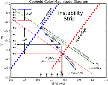
Figure 4. Color–magnitude diagram illustrating the structure of the Cepheid instability strip. Edges of the instability strip are shown by slanting, blue and red broken lines. Crossing the strip at constant period are five Cepheids represented by numbered, circled dots along a line of fixed period, having a slope β. Two reddening trajectories, through the two Cepheids defining the edges of the instability strip, are shown. They have slope RV. Projections of the Cepheids along reddening trajectories define the Wesenheit function and are seen at the top left of the figure. The ordering of the Cepheids in this projection is the same as the intrinsic ordering within the instability strip and independent of reddening. Projections of the unreddened Cepheids onto the magnitude axis preserve ordering, but become scrambled in the presence of extinction. Note Cepheid No. 2. The same comments apply to the projection onto the color axis, but note the different ordering of Cepheid No. 2 in the presence of reddening. See the text for a more complete description of this figure and its role in visualizing the method being used here to recover precision reddenings.
Download figure:
Standard image High-resolution imageFigure 4 is a color–magnitude diagram crossed by the Cepheid instability strip. The bright (blue) edge of the strip is traced by the broken thick (blue) line going diagonally to redder colors and brighter magnitudes. Similarly, the red edge is traced by the slanting thick, broken red line. A line of constant period traverses the instability strip in the middle of the plot, slanting down (to fainter magnitudes) and to the right (to redder intrinsic colors). The slope of this line of fixed period is  . Five evenly separated Cepheids (along the line of constant period) are marked across the instability strip as numbered, circled dots. Cepheid No. 1 marks the bright, blue limit of the instability strip; No. 5 is at the red edge; and No. 3 sits on the central ridge line. Additional lines of increasing period (if plotted) would be found parallel to these points, but displaced to higher luminosities and redder colors, and so on.
Marginalizations of the instability strip (i.e., orthogonal projections) can be thought of as resulting in PL and/or period–color (PC) relations. Marginalization of the color–magnitude diagram to the left axis gives rise to the Cepheid PL relation; marginalizing over magnitude and projecting down on to the color axis gives rise to the PC relation. One slice of each of these "projections" (shown at fixed period) is graphically illustrated by the horizontal displacement of our numbered points out of the instability strip to the left and onto the magnitude axis. This new distribution of points now shows the full width of the PL relation at a fixed period. The downward projection of those same Cepheids out of the instability strip and onto the color axis gives the full width of the PC relation, again at this fixed period.
The relative magnitude and/or the color ordering of the individual stars should be preserved (and identical in their order and separation) within the instability strip and for any of its projections, when intrinsic colors and magnitudes are being considered. In Figure 5 (right panel) we show that this expectation is not fulfilled for this Galactic Cepheid data set.

Figure 5. Left panel: ordering of Cepheids across the instability strip. Here we see the excellent correspondence of the relative positions of Cepheids across the strip, as measured by two independent reddening-free versions of the Wesenheit PL relation. One is based on V, (V − I) data; the other on B, (B − I) data. The correspondence is very good, with minor differences presumably being generated by photometric errors (see Figure 6). Right panel: ordering of Cepheids as traced by the W, VI PL relation in comparison to the ordering of those same Cepheids in the published B-band PL relation. Significantly more noise is seen in this comparison, suggesting that errors in the adopted reddenings are contributing to the decorrelation of the scrambling of the B-band residuals, given that the W data points are immune (by definition) to this class of errors.
Download figure:
Standard image High-resolution imageHowever, we now introduce the complicating factor of reddening (and extinction), which was the (original) focus of this paper. The shallower but still downward-sloping line (still within the instability strip, in this case) connecting Cepheid No. 2 to the point at 2' is a reddening trajectory taking the Cepheid to redder colors and fainter magnitudes, quantified by a reddening  and an extinction
  . These are conventionally related to each other by the ratio of total to selective absorption
  , which is shown in our color–magnitude diagram by the arrow passing through 2 and 2' and having a slope equal to RV.
It is important to note that RV and β are closely parallel, but they are not equal, and so their trajectories do diverge; but nevertheless the two lines are heading qualitatively in the same direction. That is, both effects (i.e., crossing the instability strip at fixed period, or being reddened) move stars to fainter magnitudes and redder colors; but in one case the effect is intrinsic to the star (and contingent on the internal structure of the Cepheid instability strip), while in the other case it is an extrinsic effect, contingent upon the amount of dust along a particular line of sight. Over the years decoupling these two effects has been problematic, but as we will now show in detail, it is not insoluble.
If we plot the magnitude residuals from the mean PL relation at each wavelength (B through K in this case) versus the corresponding (star-by-star) residuals taken from the W − log P plot,4
we should expect a one-to-one mapping of the residuals with a slope of  . If there are random errors in the adopted reddenings, they will contribute to the scatter in the fit, but only in the vertical
  direction, given that W and ΔW are both (by design) totally independent of reddening, whether those reddenings are correctly estimated or not. Within the photometric precision of the magnitudes and colors (and, for the moment, also assuming that the adopted distance moduli also have negligible random errors; but see Section 4), we can then attribute vertical deviations away from the ΔM/ΔW plot to systematic errors in the individually adopted extinctions. To gain some perspective on how these Δ–Δ plots (both Figures 5 and 6) relate back to their parent PL relations, we offer a graphical explanation in Figure 7.

Figure 6. Left panel: the photometry-induced scatter within a comparison of the individual Wesenheit magnitudes. The scatter in the points in  is only ±0.04 mag, which suggests that the precision on the uncombined photometric data points is on the order of 0.01 mag. Right panel: the same comparison as before, except with the B-band data, again suppressing the ordering in WB. Here the scatter is due to something more than photometric errors. We suggest that the source of this additional scatter is residual extinction errors.
Download figure:
Standard image High-resolution image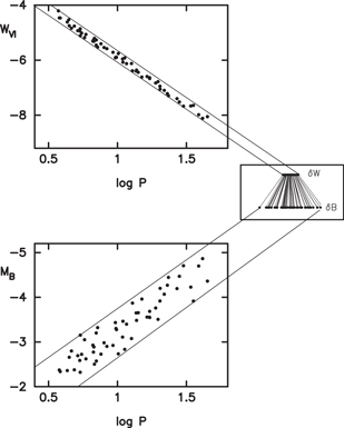
Figure 7. Graphical explanation of Figures 5 and 13. The W residuals in the right-most panel are the projections of data in the W PL relation seen (inverted) in the upper left panel. Likewise, the B-band residuals (which are connected to their respective W residuals in the right panel) are the projections of those Cepheids, as seen looking down along the B PL relation in the lower left figure.
Download figure:
Standard image High-resolution imageIf the previous assertion is the dominantly correct one, then the deviations in magnitude in the various  plots5
should all be deterministically correlated through their commonly shared, but as yet undetermined residual errors,
plots5
should all be deterministically correlated through their commonly shared, but as yet undetermined residual errors,  in their published color excesses, and they each should scale with
  ,
,  and so on. We test this assertion in Figures 8 and 9.
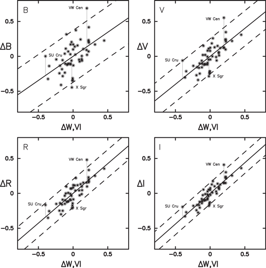
Figure 8. Multi-band correlations of the PL deviations in the optical BVR and I bandpasses (y axes), with the corresponding deviations in the W PL relation (x-axis). In the absence of errors (in distance moduli and reddenings), these plots should be highly correlated and dispersionless, since each axis is measuring the same star at the same relative position within the instability strip. However, the scatter is not random, but it is highly correlated from bandpass to bandpass, with both the overall scatter and the deviations of individual stars decreasing systematically with advancing wavelength. Several stars with some of the larges deviations (VW Cen, X Sgr, and SU Cru) are individually labelled and marked with vertical lines, indicating how much of a correction to their extinctions would be required to bring them back to the ridge line. Note the systematic decrease in the amounts of those corrections as a function of wavelength.
Download figure:
Standard image High-resolution image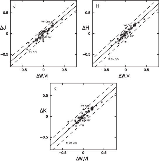
Figure 9. Same as Figure 8, except these correlations are for the near-infrared bandpasses JH and K. The further deceased dispersion of points around the ridge line is most reasonably due to the reduced sensitivity of these longer-wavelength bands to reddening and/or reddening errors.
Download figure:
Standard image High-resolution imageTo orient the reader in both anticipating and then navigating the plots appearing in Figures 11 and 12, we offer in Figure 10 a graphical illustration of the reddening and distance modulus correction procedure used here. In this figure we take the reader through one of seven such ( versus ΔW) plots considered for each of the 59 Cepheids studied here. Figure 10 plots ΔB versus ΔW. Crossing the plot from the lower left to the upper right is a thick, solid black line representing the intrinsic relation between the deterministically correlated and rank-ordered pairs of residuals from the two chosen PL relations, B − log P and W − log P, in this case. In the absence of reddening and/or distance errors (and assuminh high-precision photometry), all stars should fall somewhere along this line. However, star B, in the upper middle of the diagram, does not fall on the line, from which we must conclude that either the reddening adopted is wrong or the distance modulus is in error, or both. The broken arrow pointing straight down from B reaches the intrinsic line at point Bo. In this case, all of the error is assumed to be in the extinction, and the only correction would then be
  , as annotated to the left of the arrow. That option, however is far from unique. The arrow from B going horizontally to the left gives a second path, using a combination of distance modulus and reddening error to get back to the intrinsic line. The arrows across and down from B (both marked as
  ) show the effect of a distance error. Unlike the reddening vector in this plot, a distance error affects both axes equally. The thin solid line passing diagonally and downward to the left through star B is a line of unit slope; the two distance error arrows bring the star across and down that line. But this action does not (yet) get our star back to its intrinsic line. Indeed, it is now further from it. The addition of a new (larger) extinction correction (
 ) can then bring the star down to the intrinsic line. Similar (non-unique) trajectories are shown for star C, which also deviates from expectations, and likewise has an array of distance/extinction pairs of corrections that can return it to the line.

Figure 10. Graphical illustration of the reddening and modulus correction process. The thick solid line diagonally crossing the figure tracks the intrinsic relationship between stars in the instability strip, as measured in the Wesenheit PL relation (the x-axis) vs. their intrinsic positions in the y-axis, in this case the B-band PL relation. Points can move off of this one-to-one relation by having an incorrect distance modulus (δμ), in which case the star would move along a slope = 1 line (as shown by the thin, downward-sloping lines through examples B and C), because both W and B would be affected equally (solid arrows), independent of wavelength. Alternatively, the reddening corrections may be wrong, in which case the star will deviate (dashed arrows) vertically (by  ) from the intrinsic line, given that W is independent of reddening. For any given bandpass, the path back to the intrinsic line is not unique and can be made up of many coupled combinations of reddening and modulus corrections, as illustrated by several sample paths. The deviant stars are marked by the letters B and C. See Section 3 for a more detailed description of how the degeneracy is broken across wavelengths.
Download figure:
Standard image High-resolution image
Figure 11. Examples of the seven independent BVRIJHK residuals seen in Figures 8 and 9, each divided by their respective ratios of total to selective absorption. If the residuals are due primarily to extinction errors, then these normalized residuals should all be equal to one number, the E(B − V) correction, as shown by the horizontal dashed lines for each star. The fact that these plots are all extremely flat with wavelength gives strong support for this interpretation.
Download figure:
Standard image High-resolution imageHad there only been the B-band data to work with this degeneracy in the two corrections, they would be unbroken. However, we have seven such plots at our disposal, each of which give extinction/distance correction trajectories, and each of those trajectories has a different slope because of the differing relationships that  and so on have with ΔW. The solution for a unique value of the distance correction and its corresponding extinction correction fast becomes overdetermined by the data. And that solution resides in an eight-dimensional covariance matrix, which brings us to Figure 12. In those panels for individual Cepheids, we have collapsed six of the dimensions into one by projecting each of the multiwavelength extinction/distance trajectories into a single plane, shown by dotted straight lines of systematically decreasing slopes as a function of increasing wavelength. Under ideal circumstances (given that there is physically only one solution for the extinction and distance modulus for a given star), all of these lines should cross at a single point. In the presence of photometric noise and varying sensitivity of each of the bandpasses to extinction, the result is more likely to be a minimum dispersion region in their intersections. That expectation is realized in practice and is captured in the run of dispersion in the reddening correction, with the distance modulus correction shown in the adjacent right-hand panels for each of the stars in Figure 12.
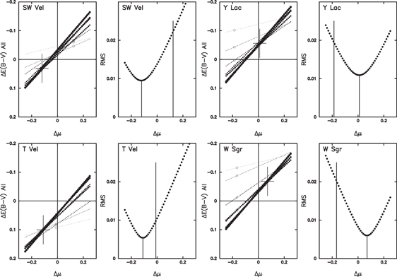
Figure 12. Four pairs of plots for individual (and representative) Cepheids showing, first, the highly covariant run of derived E(B − V) corrections as a function of assumed distance modulus corrections. Each downward-sloping line of points corresponds to a different wavelength solution. Steeper slopes come from shorter-wavelength data belying their greater sensitivity to extinction. Given the different slopes, it is inevitable that individual pairs of lines will cross; however, given that multiple crossings occur at a common position suggests more than chance is at work. Indeed, we conclude that the distance modulus at which the dispersion between the various independent band estimates reaches a minimum marks the distance modulus correction and reddening correction that should be applied to that Cepheid variable. The run of dispersion between the four shortest-wavelength estimates as a function of the distance modulus correction is shown in each of the right-hand paired panels. The minimum dispersion is marked by a short vertical line. The taller vertical line marks the raw distance modulus correction suggested by the vertical displacement of the residuals in Figures 8 and 9, before accommodating the covariant error in reddening. Similarly open circles in the left panel show the individual reddening corrections calculated for the initial estimate of the error in distance modulus, before an extensive search of parameter space (as shown in those same figures) was conducted.
Download figure:
Standard image High-resolution image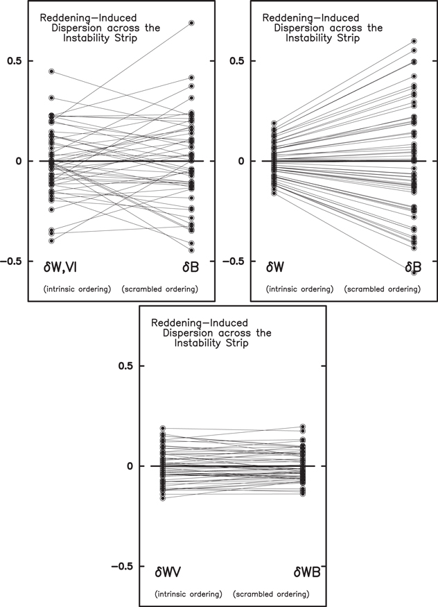
Figure 13. Top left panel: a reprise of the right-hand panel of Figure 5 showing the scrambling of data points between the intrinsic ordering of the Cepheids across the W − PL relation mapped to their noisy ordering in the B-band PL relation, before correcting for errors in their individual distance moduli and reddenings. The top right panel shows the effect of applying the modulus and reddening corrections to both the W and B PL relations. Recall that only the distance modulus corrections impact the W values; both corrections move the B-band data. The unscrambling of the B-band data is immediately obvious from the lack of lines crossing in transit. Note that the dispersion in the W relation deceased after the adjustment for individual distance moduli, while the B-band data actually increased in its calculated intrinsic dispersion. The bottom panel shows that both versions of the W − PL relation decreased in their dispersion and that the ordering of individual Cepheids across those PL relations is closely one-to-one, but still slightly scrambled by independent photometric errors, as also shown and discussed in Figure 5.
Download figure:
Standard image High-resolution imageIn the panels of Figure 11 we have plotted for each of the Cepheids their vertical scatter, taken from the  plots, divided by their corresponding wavelength-dependent values of
  . If the aforementioned vertical deviations are due to individual errors in the adopted extinctions/reddenings, then each of the "normalized residuals" (scaled by their respective wavelength-dependent values of R) should be constant as a function of wavelength; that is, their means should correspond to the
  needed to fine-tune their total color excesses. Over the seven available bands, the "normalized residual" plots for the 59 Cepheids are remarkably flat (especially for the most reddening-sensitive shorter-wavelength data; more on this as follows). This strongly supports the idea that the reddenings, as initially adopted here, are in need of adjustment and that the precision of the incoming photometry supports the determination of those adjustments.
Given the excellent agreement of these reddening estimates across wavelengths for a given Cepheid (as shown for a representative sample of Cepheids in Figure 12), and between the two independent Wesenheit determinations, we apply these "second-order corrections" to the absolute magnitudes; and perhaps more interestingly at this juncture, we apply them to the intrinsic colors. In doing this we can investigate the micro-structure of the instability strip, probing in the first instance, the slope of lines of constant period crossing the CMD. This, of course, is the color term, β, in the PLC, an example of which is given in Equation (2). Figure 13 shows the dramatic improvement in the mapping of relative positions of the Cepheids in the various PL relations originally seen to be scrambled in Figure 5.
4. Intrinsic Relations
In Table 1 we give two lines for each of the 59 Galactic Cepheids in Fouqué et al. (2007). At the beginning of the first line is the name of the Cepheid followed by the period, the  color excess, their adopted distance modulus, parallax (and quoted uncertainty), followed by their mean absolute magnitudes in the BVRI (optical), and JHK (near-infrared) bandpasses. The second line gives the updated values for all of the previously listed quantities, excluding the periods that were retained in all cases. The revised PL relations and their uncertainties, based on the corrected data in Table 1, are given in Table 2, and plotted in Figures 14–16. So as to decouple the errors quoted in the zero point from errors in the slopes, all quantities were calculated with respect to the approximate pivot point of log P = 1.0. The corrected run of slope with wavelength is shown in Figure 17. The adopted changes in reddening and distance modulus, expressed as a one-sigma dispersion, are ±0.06 and ±0.19 mag, respectively, and are shown in Figures 18 and 19 as a check on covariance and systematics.
Table 2. Galactic PL Relations for (log P = 1.0)
| Band | Slope | σ (mag) | Zero | σ(mag) | rms | rms |
|---|---|---|---|---|---|---|
| [M17] | Point | [M17] | [M17] | [F07] | ||
| (1) | (2) | (3) | (4) | (5) | (6) | (7) |
| B | −2.277 | 0.121 | −3.214 | 0.036 | 0.27 | 0.207 |
| V | −2.670 | 0.095 | −3.944 | 0.028 | 0.21 | 0.173 |
| R | −2.874 | 0.075 | −4.396 | 0.022 | 0.17 | 0.180 |
| I | −2.983 | 0.064 | −4.706 | 0.019 | 0.14 | 0.168 |
| J | −3.198 | 0.054 | −5.258 | 0.016 | 0.12 | 0.155 |
| H | −3.333 | 0.055 | −5.558 | 0.017 | 0.12 | 0.146 |
| K | −3.377 | 0.055 | −5.659 | 0.016 | 0.12 | 0.144 |
| W, VI | −3.476 | 0.037 | −5.889 | 0.011 | 0.08 | 0.168 |
| W, BI | −3.600 | 0.033 | −5.997 | 0.010 | 0.07 | 0.178 |
Download table as: ASCIITypeset image
Figure 18 shows the run of color excess corrections as a function of period of the Cepheids involved. No trend is seen, indicating that the corrections are not biasing the slope of the resulting PL relations. Similarly, Figure 19 shows a plot of the color excess corrections against the true distance modulus corrections. We expect no correlation, given the fact that the original, full reddening corrections were taken from averages over the literature and were thereby completely decoupled from the methods used in determining the parallaxes, and so any errors in the two quantities should also be decoupled, which apparently they are.
Intrinsic PL relations, based on the corrected data in Table 1, are given in equation form below. A revised and updated version of the B-band PL relation is given in Figure 14, again, explicitly marking the HST parallax sample as in Figure 1. The individual PL relations are given in the six panels of Figure 15, which are to be compared with the original plots given in Figure 2.
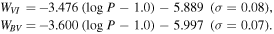

Figure 14. Corrected intrinsic PL Relation for 59 Galactic Cepheids, as measured in the B band. Cepheids with HST parallaxes from Benedict et al. (2007) are marked as large circled circles and are individually identified and labelled. Compare this with Figure 1.
Download figure:
Standard image High-resolution image
Figure 15. Corrected intrinsic PL Relation for 59 Galactic Cepheids, as measured in the VRI (first three panels) and JHK bands (final three panels). As is expected, the slopes of these PL relations increase as a function of wavelength, while the intrinsic widths of the relations systematically decrease with increasing wavelength, starting at ±0.28 mag in the B band PL relation (Figure 13) and falling to ±0.12 mag in the K band (see Table 2 for complete details).
Download figure:
Standard image High-resolution image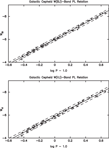
Figure 16. BI and VI reddening-free Wesenheit Period–luminosity relations for the distance modulus corrected data for 59 Galactic Cepheids. Note the strong correlation, across the two plots, of the residuals around the mean regression line functions. And note also the decreased dispersions of both relations in comparison to the uncorrected data shown in Figure 3.
Download figure:
Standard image High-resolution image
Figure 17. Run of slope of the seven Period–luminosity relations given in the text as a function of the central wavelengths of the various bands. Note the monotonic increase of slopes toward the red, asymptotically approaching a value of about −3.4 in the near-infrared (and presumably beyond). The thin dashed line gives the slope predicted by the Period–radius relation derived from Gieren et al. (1999). The near convergence of the observed slopes on this value would suggest that the influence of temperature on the slope of Cepheid PL relation is largely gone by 2 microns (K band).
Download figure:
Standard image High-resolution image
Figure 18. Run of distance modulus corrections (top) and reddening corrections (bottom) as a function of period. No correlations in either figure are seen. The one-sigma scatter is shown by two broken lines parallel to the x-axis around zero: ±0.19 mag in modulus corrections and ±0.062 mag in reddening corrections.
Download figure:
Standard image High-resolution image
Figure 19. Demonstration of the uncorrelated nature of the corrections applied here to the reddenings (x-axis) and independently to the true distance moduli (y-axis). Given that the published values were independently determined, it is perfectly reasonable to expect that the corrections would be largely uncorrelated, as they appear to be. The formal fit, as shown, has a slope of −0.64 ± 0.39.
Download figure:
Standard image High-resolution imageBelow we give the PLC relations for MV and all six of the independent colors. The quoted sigmas are consistent with photometric errors on the photometry, amounting to  mag,
mag,  mag, and
  mag. However, it is interesting to note that the V-band PLC has a sigma of only 0.06 mag, meaning that if independent reddenings can be obtained, this formula is capable of delivering distances to Cepheids that are individually good to ±3%. Magnitude versus color residual plots leading to the color terms in these equations are given in Figure 20.
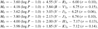
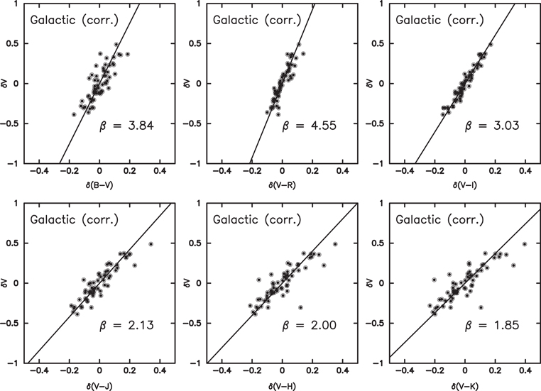
Figure 20. Slopes of lines of constant period crossing the Cepheid instability strip in all six of the exemplary color–magnitude diagrams made up from the BVRIJHK photometry. The slopes are given in the lower right portions of each of the figures, derived from the fits shown as solid lines through the highly correlated residuals from the respective period–luminosity and period–color relations. Note the exceptionally tight scatter in the upper right V vs. (V–I) plot. Residual scatter in these plots reflects the precision of published photometry.
Download figure:
Standard image High-resolution image5. Conclusions
We have introduced and applied a novel technique for refining the individual distances and line-of-sight reddenings to Galactic Cepheids. Starting with the reddening-independent Wesenheit function, it is possible to order individual Cepheids by their position within and across the instability strip. Demanding the same relative ordering across the corresponding projections of the instability strip into the multiwavelength PL relations reveals discrepancies in the ordering that can be corrected by applying differential corrections to their true distance moduli and their published reddenings. By minimizing the scatter in the adopted reddening as a function of the reddening-independent, true distance modulus, updated parallaxes, and reddenings can be obtained on a star-by-star basis, self-consistently determined across seven optical and near-infrared bands. The resulting PL relations, updated in this way, show the expected monotonic increase of slope and corresponding monotonic decrease in width as a function of increasing wavelength of the observations. Residuals measured from the ridge lines of the multiwavelength PL relations are highly correlated (again as expected), revealing the intrinsic PLC relation underwriting the individual PL relations.
We thank the Carnegie Institution for Science and the University of Chicago for their continuing generous support of our long-term research into the expansion rate of the universe. We also thank Dylan Hatt for careful and insightful reading of an early draft of this paper. Finally, we are indebted to the referee for their careful reading of the paper and the many detailed suggestions offered that made the final paper more readable, and for strongly urging us to describe Figure 11, which is at the heart of the process by which our finally adopted values of extinctions and distances were self-consistently derived.
Footnotes
- 3
It should be noted that van den Bergh (1975) had earlier used a similar combination of magnitude and color as a means of cancelling out the change of absolute magnitude as a function of intrinsic color as one traverses the Cepheid instability strip, by using the slope of lines of constant period in the color–magnitude diagram. He did this by scaling the
 color by a factor of 2.67 and subtracting that from the apparent V magnitude to get a magnitude that was designed to be insensitive to its intrinsic position within the instability strip, assuming that the multiplicative factor (the color term in the PLC) was known a priori.
 - 4
For consistency with the Fouqué et al. (2007) paper, we adopt their two versions of the Wesenheit function:
and . - 5
These types of residual-residual plots date at least as far back as to Sandage & Tammann (1968, 1969, Figures 2 and 6, respectively), and are more widely seen in Sandage (1972), Figure 4. subsequent applications include Figure 3 in Madore (1982), Figure 3 in Beaulieu et al. (2001), and most recently, Figure 14 in Macri et al. (2015).


