


ABSTRACT
We present optical, near-infrared, and radio observations of the afterglow of GRB 120521C. By modeling the multi-wavelength data set, we derive a photometric redshift of z ≈ 6.0, which we confirm with a low signal-to-noise ratio spectrum of the afterglow. We find that a model with a constant-density environment provides a good fit to the afterglow data, with an inferred density of n ≲ 0.05 cm−3. The radio observations reveal the presence of a jet break at tjet ≈ 7 d, corresponding to a jet opening angle of θjet ≈ 3°. The beaming-corrected γ-ray and kinetic energies are Eγ ≈ EK ≈ 3 × 1050 erg. We quantify the uncertainties in our results using a detailed Markov Chain Monte Carlo analysis, which allows us to uncover degeneracies between the physical parameters of the explosion. To compare GRB 120521C to other high-redshift bursts in a uniform manner we re-fit all available afterglow data for the two other bursts at z ≳ 6 with radio detections (GRBs 050904 and 090423). We find a jet break at tjet ≈ 15 d for GRB 090423, in contrast to previous work. Based on these three events, we find that γ-ray bursts (GRBs) at z ≳ 6 appear to explode in constant-density environments, and exhibit a wide range of energies and densities that span the range inferred for lower redshift bursts. On the other hand, we find a hint for narrower jets in the z ≳ 6 bursts, potentially indicating a larger true event rate at these redshifts. Overall, our results indicate that long GRBs share a common progenitor population at least to z ∼ 8.
Export citation and abstract BibTeX RIS
1. INTRODUCTION
Long duration γ-ray bursts (GRBs) are known to be associated with the violent deaths of massive stars (e.g., Woosley & Bloom 2006). In conjunction with the large luminosities of their afterglows, they can therefore serve as powerful probes of the high-redshift universe (Inoue et al. 2007), providing clues to the formation environments of the first stars, the ionization and metal enrichment history of the universe, and the properties of galaxies that are otherwise too faint to study through direct imaging and spectroscopy (Totani et al. 2006; Tanvir et al. 2012; Chornock et al. 2013). Furthermore, modeling of multi-wavelength afterglow data allows us to constrain the densities and structure of massive star environments on parsec scales, as well as the energies of the explosions and the degree of ejecta collimation.
To use GRBs as effective probes of star-formation in the re-ionization era (z ≳ 6; Fan et al. 2002, 2006), it is important to understand whether there is any evolution in the properties of their progenitors with redshift. This is best achieved by studying the afterglows of the highest-redshift events to determine their explosion energy, circumburst density and degree of collimation, and by comparing these properties with those of their lower-redshift counterparts. In the long term, such studies have the potential to uncover the contribution of Population III stars, which have been speculated to be highly energetic (Eiso ∼ 1052–1057 erg) with relatively long durations (T90 ∼ 1000 s; e.g., Fryer et al. 2001; Bromm et al. 2003; Heger et al. 2003; Mészáros & Rees 2010; Suwa & Ioka 2011; Toma et al. 2011; Wang et al. 2012).
At present, there are only three GRBs with spectroscopically confirmed redshifts of z ≳ 6: GRB 050904 at z = 6.29 (Tagliaferri et al. 2005; Haislip et al. 2006; Kawai et al. 2006), GRB 080913 at z = 6.70 (Greiner et al. 2009), and GRB 090423 at z = 8.23 (Salvaterra et al. 2009; Tanvir et al. 2009). In addition, GRB 090429B has an inferred photometric redshift of z ∼ 9.4 (Cucchiara et al. 2011). To fully determine the physical properties of a GRB and its environment requires multi-wavelength observations spanning the radio through to the X-rays; only two of the z ≳ 6 events have radio detections: GRB 050904 (Frail et al. 2006; Gou et al. 2007) and GRB 090423 (Tanvir et al. 2009; Chandra et al. 2010).
Previous studies of GRB 050904 have found a high circumburst density (n ∼ 102–103 cm−3; Frail et al. 2006; Gou et al. 2007), a high isotropic-equivalent γ-ray energy (Eγ, iso ≈ 1054 erg; Cusumano et al. 2006), a large isotropic-equivalent kinetic energy (EK, iso ≈ few × 1053 erg; Frail et al. 2006; Gou et al. 2007), and no evidence for host extinction (AV ≲ 0.1 mag; Gou et al. 2007; Zafar et al. 2010, although see also Stratta et al. 2007, 2011). A jet break at tjet ≈ 3 d (Tagliaferri et al. 2005) indicates a beaming-corrected γ-ray energy of 8 × 1051 erg and kinetic energy of EK ≈ 2 × 1051 erg, the latter being one of the largest known (Gou et al. 2007). GRB 090423 has an inferred density of n ≲ 1 cm−3 (Chandra et al. 2010), large isotropic-equivalent γ-ray energy (Eγ ≳ 1053 erg) and kinetic energy (EK, iso ≳ 3 × 1053 erg), and no host extinction (AV ≲ 0.1 mag; Tanvir et al. 2009). No jet break was seen for this event, resulting in a claim of EK ≳ 7 × 1051 erg, even larger than for GRB 050904.
Whereas individual studies of these two GRBs have been undertaken, they employed different implementations of afterglow synchrotron models and their results cannot be compared directly. Here we report multi-wavelength observations of GRB 120521C and deduce a photometric redshift of z ≈ 6, making this the third high-redshift GRB with multi-wavelength data from radio to X-rays. The availability of well-sampled light curves spanning several orders of magnitude in frequency and time allow us to perform broadband afterglow modeling, and thereby to determine the energetics of the explosion, the density profile of the circumburst environment, the microphysical parameters of the relativistic shocks, and the collimation of the ejecta. We additionally re-analyze all available afterglow data for GRBs 050904 and 090423, enabling us to compare the three high-redshift GRBs in a uniform manner. Finally, we compare the properties of the high-redshift GRBs to those of bursts at z ∼ 1 to investigate whether high-redshift GRBs exhibit evidence for an evolution in the progenitor population or favor different environments than their lower-redshift counterparts. We present our observations and analysis for GRB 120521C in Section 2 and determine a photometric redshift for this event in Section 3. We describe the theoretical model employed and our multi-wavelength modeling software in Section 4 and present our broadband afterglow model for GRB 120521C in Section 5. We apply our modeling code to re-derive the properties of GRBs 050904 and 090423 in Section 6 and compare the results to those obtained for GRB 120521C and to lower-redshift events in Section 7. We present our conclusions in Section 8. We use the standard cosmological parameters, Ωm = 0.27, ΩΛ = 0.73 and H0 = 71 km s−1 Mpc−1. All magnitudes are in the AB system, unless stated otherwise.
2. GRB PROPERTIES AND OBSERVATIONS
GRB 120521C was discovered with the Swift Burst Alert Telescope (BAT; Barthelmy et al. 2005) on 2012 May 21 at 23:22:07 UT (Baumgartner et al. 2012). The burst duration was T90 = (26.7 ± 0.4) s, with a fluence of Fγ = (1.1 ± 0.1) × 10−6 erg cm−2 (15–150 keV; Markwardt et al. 2012). The Swift X-Ray Telescope (XRT; Burrows et al. 2005) began observing the field 69 s after the BAT trigger, leading to the detection of an X-ray afterglow at coordinates R.A.(J2000) = 14h17m08 73, Decl.(J2000) = +42°08'41
 0, with an uncertainty radius of 16 (90% containment).7 XRT continued observing the afterglow for 1.5 days in photon counting (PC) mode, with the last detection at about 0.5 days.
2.1. X-Rays
We analyzed the XRT data using the latest version of the HEASOFT package (v6.11) and corresponding calibration files. We utilized standard filtering and screening criteria, and we generated a count-rate light curve following the prescriptions by Margutti et al. (2010). The data were re-binned with the requirement of a minimum signal-to-noise ratio of 4 in each temporal bin.
We used Xspec (v12.6) to fit the PC-mode spectrum between 3 × 10⁻³ and 0.35 d, assuming a photoelectrically absorbed power law model (tbabs × ztbabs × pow) and a Galactic neutral hydrogen column density of NH, MW = 1.1 × 1020 cm−2 (Kalberla et al. 2005), fixing the source redshift at z = 6.0 (see Sections 3 and 5). Our best-fit model has a photon index of  (68% confidence intervals, C-stat = 151 for 180 degrees of freedom). We found no evidence for additional absorption with a 3σ upper limit of NH, int ≲ 6.6 × 1022 cm−2, assuming solar metallicity.
To assess the impact of the uncertain intrinsic absorption, we fit a PC-mode spectrum with the intrinsic NH fixed to this 3σ upper limit and found Γ = 2.03 ± 0.26. Next, we fixed the intrinsic absorption to zero and found Γ = 1.77 ± 0.21. The two light curves differ by less than 5%. In the following analysis, we assume NH, int = 0 and use the corresponding computed 0.3–10 keV light curve, together with Γ = 1.77 to compute the 1 keV flux density (Table 1).
Table 1. Swift XRT Observations of GRB 120521C
| Δt | Flux Density | Uncertainty | Detection? |
|---|---|---|---|
| (days) | (mJy) | (mJy) | (1 = Yes) |
| 0.205 | 0.000137 | 5.19e-05 | 1 |
| 0.312 | 5.73e-05 | 2.21e-05 | 1 |
| 0.581 | 2.08e-05 | 6.94e-06 | 1 |
| 1.25 | 2.99e-05 | 9.98e-06 | 0 |
Download table as: ASCIITypeset image
2.2. Optical and Near-IR
We obtained riz-band imaging of the XRT error circle beginning about 40 min after the BAT trigger using ACAM on the William Herschel Telescope (WHT) and MOSCA on the Nordic Optical Telescope (NOT). We analyzed the data using standard procedures within IRAF8 and astrometrically aligned and photometrically calibrated the images using Sloan Digital Sky Survey (SDSS) stars in the field. We found a brightening point source in the WHT z-band images within the revised XRT error circle at the position R.A.(J2000) = 14h17m0882, Decl.(J2000) = +42°08'416, with z = 23.5 ± 0.3 mag9 (at Δt ≈ 0.04 d), i ≳ 23.8 mag (3σ), and r ≳ 24.3 mag (3σ; Table 2).
Table 2. Optical and Near-infrared Observations of GRB 120521C
| Δt | Telescope | Instrument | Band | Frequency | Flux densitya | Uncertaintya | Detection? |
|---|---|---|---|---|---|---|---|
| (days) | (Hz) | (mJy) | (mJy) | (1 = Yes) | |||
| 0.0316 | WHT | ACAM | R | 4.81e+14 | 0.000585 | 0.000195 | 0 |
| 0.0372 | WHT | ACAM | I | 3.93e+14 | 0.00109 | 0.000362 | 0 |
| 0.0379 | NOT | R | 4.81e+14 | 0.000702 | 0.000234 | 0 | |
| 0.0405 | WHT | ACAM | z | 3.46e+14 | 0.00146 | 0.000408 | 1 |
| 0.0433 | NOT | I | 3.93e+14 | 0.00135 | 8.00e-05 | 0 | |
| 0.106 | WHT | ACAM | z | 3.46e+14 | 0.00444 | 0.000555 | 1 |
| 0.108 | WHT | ACAM | z | 3.46e+14 | 0.00369 | 0.000669 | 1 |
| 0.109 | WHT | ACAM | z | 3.46e+14 | 0.00476 | 0.000615 | 1 |
| 0.111 | WHT | ACAM | z | 3.46e+14 | 0.0036 | 0.000625 | 1 |
| 0.112 | WHT | ACAM | z | 3.46e+14 | 0.00402 | 0.000651 | 1 |
| 0.115 | WHT | ACAM | z | 3.46e+14 | 0.00313 | 0.000717 | 1 |
| 0.117 | WHT | ACAM | z | 3.46e+14 | 0.00398 | 0.000653 | 1 |
| 0.119 | WHT | ACAM | z | 3.46e+14 | 0.00253 | 0.000748 | 1 |
| 0.12 | WHT | ACAM | z | 3.46e+14 | 0.00408 | 0.000635 | 1 |
| 0.122 | WHT | ACAM | z | 3.46e+14 | 0.0031 | 0.000725 | 1 |
| 0.124 | WHT | ACAM | z | 3.46e+14 | 0.00301 | 0.000649 | 1 |
| 0.126 | WHT | ACAM | z | 3.46e+14 | 0.00300 | 0.00068 | 1 |
| 0.208 | PAIRITEL | K | 1.37e+14 | 0.255 | 0.0848 | 0 | |
| 0.208 | PAIRITEL | H | 1.84e+14 | 0.0932 | 0.031 | 0 | |
| 0.208 | PAIRITEL | J | 2.38e+14 | 0.0633 | 0.0211 | 0 | |
| 0.282 | UKIRT | WFCAM | K | 1.37e+14 | 0.0125 | 0.00134 | 1 |
| 0.318 | UKIRT | WFCAM | J | 2.38e+14 | 0.0112 | 0.00108 | 1 |
| 0.321 | Gemini-North | GMOS | z | 3.46e+14 | 0.00632 | 0.000316 | 1 |
| 0.324 | Gemini-North | GMOS | z | 3.46e+14 | 0.00664 | 0.000332 | 1 |
| 0.326 | Gemini-North | GMOS | z | 3.46e+14 | 0.00659 | 0.000329 | 1 |
| 0.329 | Gemini-North | GMOS | z | 3.46e+14 | 0.00601 | 0.000301 | 1 |
| 0.332 | Gemini-North | GMOS | z | 3.46e+14 | 0.00686 | 0.000343 | 1 |
| 0.334 | Gemini-North | GMOS | z | 3.46e+14 | 0.00627 | 0.000313 | 1 |
| 0.336 | Gemini-North | GMOS | z | 3.46e+14 | 0.00623 | 0.000311 | 1 |
| 0.339 | Gemini-North | GMOS | z | 3.46e+14 | 0.00553 | 0.000277 | 1 |
| 0.341 | Gemini-North | GMOS | z | 3.46e+14 | 0.00647 | 0.000323 | 1 |
| 0.344 | Gemini-North | GMOS | z | 3.46e+14 | 0.00604 | 0.000302 | 1 |
| 0.347 | Gemini-North | GMOS | z | 3.46e+14 | 0.00593 | 0.000296 | 1 |
| 0.349 | Gemini-North | GMOS | z | 3.46e+14 | 0.00594 | 0.000297 | 1 |
| 0.352 | Gemini-North | GMOS | z | 3.46e+14 | 0.00619 | 0.00031 | 1 |
| 0.354 | Gemini-North | GMOS | z | 3.46e+14 | 0.00569 | 0.000284 | 1 |
| 0.356 | UKIRT | WFCAM | H | 1.84e+14 | 0.0126 | 0.00135 | 1 |
| 0.514 | Keck | LRIS | g | 6.29e+14 | 0.000114 | 3.8e-05 | 0 |
| 0.516 | Keck | LRIS | I | 3.93e+14 | 0.000453 | 0.000151 | 0 |
| 0.579 | Gemini-North | GMOS | I | 3.93e+14 | 0.000495 | 0.000165 | 0 |
| 0.586 | Gemini-North | GMOS | z | 3.46e+14 | 0.00433 | 0.000374 | 1 |
| 1.05 | WHT | ACAM | z | 3.46e+14 | 0.00191 | 0.000108 | 1 |
Note. aNot corrected for Galactic extinction.
Download table as: ASCIITypeset image
Given the red color of the afterglow, r − z ≳ 0.8 mag, we considered this to be a possible high redshift source, and thus triggered a sequence of optical and infrared imaging with the Gemini-North Multi-Object Spectrograph (GMOS) on Gemini-North (iz), the Low Resolution Imaging Spectrometer (LRIS) on the W. M. Keck telescope (gI), and the Wide-Field Camera (WFCAM) on the United Kingdom Infrared Telescope (UKIRT; JHK). We reduced the data in the standard manner, using the instrument pipelines for GMOS and WFCAM. We performed aperture photometry using the Graphical Astronomy and Image Analysis tool (GAIA). We placed the aperture with reference to the GMOS z-band image with the highest signal-to-noise detection of the afterglow, and used an aperture size appropriate to the seeing FWHM. We determined the level and variance of the sky background from about 20 same-sized apertures placed on sky regions proximate to the burst location. We calibrated the optical photometry to SDSS and the JHK photometry using Two Micron All Sky Survey stars in the field.
We detected the afterglow in all filters redward of z-band and obtained non-detections with deep limits in the optical filters (gri) at the level of Fν ≲ 0.45 μJy (3σ; Figure 1 and Table 2). On the other hand, the infrared colors were relatively blue: J − H = 0.13 ± 0.21 mag and J − K = 0.12 ± 0.21 mag. This suggested that reddening due to dust was negligible, and that the red r − z color was due to the Lyα break falling within the z-band, implying a photometric redshift of z ∼ 6. We perform a full analysis to determine a photometric redshift in Section 3.

Figure 1. Optical and near-infrared observations of GRB 120521C. The refined XRT position is marked by the white circle (16 radius). The afterglow is detected in z-band with Gemini/GMOS and WHT/ACAM and in JHK imaging with UKIRT/WFCAM (Table 2) but is undetected at both R- and I-band.
Download figure:
Standard image High-resolution imageThe Swift UV/Optical Telescope (UVOT) began observing the field 77 s after the burst. No optical counterpart was detected at the location of the X-ray afterglow (Oates & Baumgartner 2012). We performed photometry using the HEASOFT task uvotsource at the location of the NIR afterglow, and report our derived upper limits in Table 3.
Table 3. Swift UVOT Observations of GRB 120521C
| Δt | Filter | Frequency | 3σ Flux Upper Limita |
|---|---|---|---|
| (days) | (Hz) | (mJy) | |
| 1.5907e-02 | B | 6.9250e+14 | 2.8387e-02 |
| 1.6055e-02 | UVM2 | 1.3450e+15 | 1.3113e-02 |
| 1.4277e-02 | U | 8.5630e+14 | 9.5506e-03 |
| 1.6770e-02 | V | 5.5500e+14 | 5.4590e-02 |
| 1.7337e-02 | UVW1 | 1.1570e+15 | 9.5866e-03 |
| 1.6487e-02 | UVW2 | 1.4750e+15 | 8.7097e-03 |
| 1.3334e-02 | WHITE | 8.6400e+14 | 3.7121e-03 |
| 1.0321e-01 | B | 6.9250e+14 | 1.3541e-02 |
| 7.4747e-02 | UVM2 | 1.3450e+15 | 1.0309e-02 |
| 1.4464e-01 | U | 8.5630e+14 | 8.6864e-03 |
| 2.0687e-01 | V | 5.5500e+14 | 4.6748e-02 |
| 1.4259e-01 | UVW1 | 1.1570e+15 | 3.8169e-03 |
| 2.0528e-01 | UVW2 | 1.4750e+15 | 1.9738e-03 |
| 1.0784e-01 | WHITE | 8.6400e+14 | 2.9149e-03 |
| 5.7824e-01 | WHITE | 8.6400e+14 | 8.9244e-04 |
| 1.5257e+00 | UVM2 | 1.3450e+15 | 1.5728e-03 |
Note. aNot corrected for Galactic extinction.
Download table as: ASCIITypeset image
We obtained spectroscopic observations of the afterglow with Gemini-North/GMOS beginning 1.03 d post-burst for a total exposure of 3600 s, by which time the source had faded to z ≈ 23.2 mag. We used the R400 grism and a slit width of 1'', providing a wavelength coverage of 5850–10140 Å and a resolution of R ≈ 1900. The data were reduced using the GMOS pipeline. A faint trace of the afterglow was visible at the red end of the spectrum. The trace disappears around 8700 Å, which unfortunately coincides with the gap between the GMOS CCDs. Assuming this break is due to Lyα, we deduce z ≈ 6.15, consistent with the red r − z color. We plot the extracted spectrum in Figure 2, adaptively re-binned to produce approximately the same noise in each bin.

Figure 2. 1D (top) and 2D (bottom) Gemini-North/GMOS spectrum of GRB 120521C obtained 1.03 d. after the burst. The blue box indicates the extraction region in the 2D spectrum, located using the trace of a reference star. The flux from the afterglow disappears blueward 8700 Å, coincident with a chip gap, and is weakly detected at redder wavelengths. Assuming this break is due to Lyα, we find a redshift of z ∼ 6.15.
Download figure:
Standard image High-resolution image2.3. Radio
We observed GRB 120521C with the Karl G. Jansky Very Large Array (VLA) beginning on 2012 May 22.12 UT at mean frequencies of 5.8 GHz (lower and upper sideband frequencies set at 4.9 and 6.7 GHz, respectively) and 21.8 GHz (lower and upper sideband frequencies of 19.1 and 24.4 GHz, respectively). We employed 3C286 as a flux and bandpass calibrator and interleaved observations of J1419+3821 for calculating time-dependent antenna gains. All observations utilized the VLA WIDAR correlator (Perley et al. 2011). We excised radio frequency interference from the data, resulting in final effective bandwidths of ≈1.5 GHz at 5.8 GHz and ≈1.75 GHz at 21.8 GHz. We performed all data calibration and analysis with the Astronomical Image Processing System (AIPS; Greisen 2003) using standard procedures for VLA data reduction.
In our first epoch at 21.8 GHz (0.15 d after the burst), we did not detect any significant radio emission within the refined Swift XRT error circle to a 3σ limit of 50 μJy (Table 4). However, we detected a radio source in the second epoch at 1.15 d after the burst (Figure 3). This source subsequently faded, confirming it as the radio afterglow. We also detected the afterglow at 6.7 GHz in our observations taken between 4.25 and 29.25 d after the burst; however, we did not find significant radio emission at 4.9 GHz. We treat these two side-bands separately in our analysis, but for simplicity, we show side-band averaged images in Figure 4.

Figure 3. VLA observations of GRB 120521C at a mean frequency of 21.8 GHz. The refined XRT position is indicated by the white circle (16 radius). The arrow marks the radio afterglow when detected. The last image is a stack of the data at 12.3 and 14.3 d with a marginal detection at ∼3σ (see Table 4 for details).
Download figure:
Standard image High-resolution image
Figure 4. VLA observations of GRB 120521C at a mean frequency of 5.8 GHz. The refined XRT position is marked by the white circle (16 radius). Crosses indicate the mean position of the GRB from our 21.8 GHz observations (see Figure 3).
Download figure:
Standard image High-resolution imageTable 4. VLA Observations of GRB 120521C
| Δt | VLA | Frequency | Integration Time | Integrated Flux | Uncertainty | Detection? |
|---|---|---|---|---|---|---|
| (days) | Configuration | (GHz) | (min) | density (μJy) | (μJy) | (1 = Yes) |
| 0.15 | CnB | 4.9 | 15.28 | 41.7 | 13.9 | 0 |
| 6.7 | 15.28 | 48.0 | 16.0 | 0 | ||
| 21.8 | 15.07 | 50.7 | 16.9 | 0 | ||
| 1.15 | CnB | 4.9 | 10.12 | 51.0 | 17.0 | 0 |
| 6.7 | 10.12 | 57.3 | 19.1 | 0 | ||
| 21.8 | 15.07 | 112 | 18.5 | 1 | ||
| 4.25 | B | 4.9 | 15.27 | 41.1 | 13.7 | 0 |
| 6.7 | 15.27 | 54.5 | 14.3 | 1 | ||
| 21.8 | 14.52 | 66.5 | 18.6 | 1 | ||
| 7.25 | B | 4.9 | 15.12 | 39.9 | 13.3 | 0 |
| 6.7 | 15.12 | 48.8 | 14.2 | 1 | ||
| 21.8 | 12.97 | 65.8 | 18.3 | 1 | ||
| 12.27 | B | 21.8 | 32.95 | 30.6 | 10.2 | 0 |
| 14.27 | B | 21.8 | 32.68 | 38.4 | 12.8 | 0 |
| 13.27a | B | 21.8 | ... | 26.2 | 9.2 | 1 |
| 29.25 | B | 4.9 | 24.87 | 35.7 | 11.9 | 0 |
| 6.7 | 24.87 | 29.1 | 9.7 | 1 | ||
| 174.66 | A | 4.9 | 46.43 | 28.5 | 9.5 | 0 |
| A | 6.7 | 46.43 | 23.4 | 7.8 | 0 |
Note. aWeighted sum of data at 12.27 and 14.27 d.
Download table as: ASCIITypeset image
We used the AIPS task JMFIT to determine the positional centroid and integrated flux of the radio afterglow in each epoch by fitting a Gaussian at the position of the source and fixing the source size to the restoring beam shape. The weighted mean position of the source, determined by combining all 21.8 GHz detections is R.A.(J2000) = 14h17m08803 ± 0002, Decl.(J2000) = +42°08' 4121 ± 003 (1σ). We summarize the results of the radio observations in Table 4. GRB 120521C was also observed by the Arcminute Microkelvin Imager Large Array at 15.75 GHz (AMI-LA; Staley et al. 2013), and we include the reported upper limits in our analysis.
3. PHOTOMETRIC REDSHIFT
To determine a photometric redshift, we interpolate the optical and NIR observations to a common time. To minimize this interpolation, we select a time of 8.1 hr after the burst when we obtained near-simultaneous zJHK photometry. We perform a weighted sum of the GMOS z-band observations at 7.7 hr <Δt < 8.5 hr and find Fν = 6.22 ± 0.05 μJy at Δt ≈ 8.1 h. Since the NIR light curves are not well-sampled before 1 d, we use the z-band light curve to extrapolate the NIR fluxes. We first fit the z-band light curve with a broken power-law of the form  , where tb is the break time, Fb is the flux at the break time, α1 and α2 are the temporal decay rates before and after the break, respectively, and s is the sharpness of the break.10 We use the Python function curve_fit to estimate these model parameters and the associated covariance matrix. Our best-fit parameters are tb = (0.34 ± 0.07) d, Fb = 6.89 μJy, α1 = 0.83 ± 0.31, α2 = −1.38 ± 0.43, and s = 1.7 ± 1.6 (Figure 5). Using this model to extrapolate the JHK photometry, we obtain Fν = 11.1 ± 1.1 μJy, 12.8 ± 1.4 μJy, and 12.4 ± 1.3 μJy, at J, H, and K band, respectively, at the common time of 8.1 hr. The uncertainties are statistical only and do not include the systematic uncertainties introduced by the interpolation, which are less than 2%.

Figure 5. z-band light curve of GRB 120521C. The solid line is the best-fit broken-power-law model described in Section 5.1.
Download figure:
Standard image High-resolution imageAfter obtaining NIR fluxes at a common time, we build a composite model for the afterglow spectral energy distribution (SED). We use a sight-line-averaged model for the optical depth of the intergalactic medium (IGM) as described by Madau (1995), accounting for Lyα absorption by neutral hydrogen along the line of sight and photoelectric absorption by intervening systems. We also include Lyα absorption by the host galaxy, for which we assume a column of log (NH/cm−2) = 21.1, the mean value for GRBs at z ∼ 1 (Fynbo et al. 2009). The free parameters in our model are the redshift of the GRB, the extinction along the line of sight within the host galaxy (AV), and the spectral index (β) of the afterglow SED, Fν∝νβ. In order to not bias our results, we assume a uniform prior for the redshift and the extinction. We further use the distribution of extinction-corrected spectral slopes, βox from Greiner et al. (2011) as a prior on β. We use a Markov Chain Monte Carlo (MCMC) algorithm to explore the parameter space, integrating the model over the filter bandpasses and computing the likelihood of the model by comparing the resulting fluxes with the observed values. Details of our MCMC implementation are described in Section 4.2.
We find  ,
,  , and
, and  mag, where the uncertainties correspond to 68% credible intervals about the median.11 The parameters of the highest-likelihood model are z = 6.03, β = −0.34, and AV = 0 mag, consistent with the 68% credible intervals derived from the posterior density functions (Table 5). We note that the median values differ from the highest-likelihood values. This is a standard feature of Monte Carlo analyses whenever the likelihood function is asymmetric about the highest-likelihood point. In this case, this occurs because the extinction is constrained to be positive, resulting in a truncation of parameter space. The best-fit model and a model with the median parameters are plotted in Figure 6, while the full posterior density function for the redshift is shown in Figure 7. We can rule out a redshift of z ≲ 5.6 at 99.7% confidence. The corresponding 99.7% confidence upper limit is z ≲ 6.2.

Figure 6. Optical-to-NIR spectral energy distribution of GRB 120521C at 8.1 hr. The z-band data point is a weighted average of all Gemini-North/GMOS frames taken at 7.7–8.5 hr. (see Figure 5). The JHK photometry has been extrapolated from the nearest detections using the best-fit z-band light curve (Figure 5), while the g and i upper limits are from Keck at ≈12.2 h, used without extrapolation (Table 2). The data points have been placed at the centroid of the filter bandpass for clarity. The lines are models for the afterglow SED, including IGM and ISM absorption, using the best-fit (highest-likelihood) model (solid), and the median values of the parameter distributions (dashed; Table 5). We show the 1σ, 2σ, and 3σ contours for the correlation between extinction (AV) and redshift (z) in the inset. The black dot indicates the best-fit model with no extinction and z ≈ 6.0.
Download figure:
Standard image High-resolution image
Figure 7. Posterior density function for the redshift of GRB 120521C from fitting the SED at 8.1 hr. (orange; see Figure 6), and from fitting all available afterglow data with the redshift as a free parameter, using ISM (blue) and wind (green) models. The vertical lines indicate the redshifts of the best-fit models.
Download figure:
Standard image High-resolution imageTable 5. Parameters from Optical/NIR SED Modeling of GRB 120521C
| Parameter | Best-fit | 68% Credible Regions |
|---|---|---|
| z | 6.03 | 5.93 |
| β | −0.34 |  |
| AV | 0 | 0.11 |
Download table as: ASCIITypeset image
We note that this constraint on the redshift relies on the assumed prior for β. Using broadband modeling we can locate the synchrotron break frequencies (explained in the next section) and thereby constrain β independent of the redshift. Therefore, in the subsequent multi-wavelength modeling we leave the redshift as a free parameter and fit for it along with the parameters of the explosion. For the optical and NIR frequencies, we integrate the model over the filter bandpasses to take into account absorption by the intervening IGM and the interstellar medium (ISM) of the host galaxy.
4. MULTI-WAVELENGTH MODELING
4.1. Synchrotron Model
In the standard synchrotron model of GRB afterglows, the SED consists of multiple power-law segments delineated by "break-frequencies," namely, the synchrotron cooling frequency (νc), the typical synchrotron frequency (νm), and the self-absorption frequency (νa). The location and evolution of these break frequencies, and the overall normalization of the spectrum depend upon the physical parameters of the explosion: the energy (EK, iso), the circumburst density (n0, or the normalized mass-loss rate in a wind environment, A*), the power-law index of the electron energy distribution (p), the fraction of the blastwave energy transferred to relativistic electrons ( e) and to the magnetic fields (B), and the half-angle of the collimated outflow (θjet). For further details of the synchrotron model, see Sari et al. (1998).
We have developed Python software for broadband modeling of GRB afterglows. Our software implements the full afterglow model with smoothly connected power law segments presented in Granot & Sari (2002, henceforth GS02). The model includes synchrotron cooling and self-absorption for both ISM and wind-like environments. The full treatment of the synchrotron model including local electron cooling results in five different spectral regimes with 11 definitions of the break frequencies, corresponding to different orderings of the synchrotron frequencies. Depending on the circumburst density profile and the combination of physical parameters, the spectrum evolves from fast cooling (νc < νm) to slow cooling (νc > νm), transitioning through the various spectral regimes (Figure 2 in GS02).
Given a set of explosion parameters, we compute the location of each of the 11 break frequencies using the expressions in GS02. Owing to slightly different normalizations of the break frequencies between the five spectral regimes, a sharp transition from one spectrum to another sometimes introduces discontinuities in the light curves. This is exacerbated by the fact that the transition times between spectra are not uniquely defined (see Table 3 in GS02). To overcome this and to establish a consistent framework, we add a linear combination of all spectra through which the spectrum evolves for a given set of physical parameters, with time-dependent weights. These weights are chosen such that each spectrum dominates in its own regime of validity, while allowing for the light curves to remain smooth when break frequencies cross each other at spectral transitions. A detailed description of our weighting scheme is provided in Appendix A.
The hydrodynamics presented in GS02 assume spherical expansion. While this is a good approximation in the early phase of the afterglow evolution when the Lorentz factor of the ejecta is  and only a small fraction of the jet is visible to an observer on Earth, deceleration of the jet to
  results in a steep decline in the observed flux density at all frequencies at later times. We account for this "jet break" by changing the evolution of the break frequencies after the break time, tjet, using the prescription in Sari et al. (1999), smoothing over the transition with a smoothing parameter12 (for further discussion of the jet break based on numerical simulations, see van Eerten & MacFadyen 2012 and Leventis et al. 2013).
Our software also accounts for possible contributions in the optical and NIR from the host galaxy, as well as absorption and reddening of the afterglow light by dust in the host. For the former, we add the contribution of the host to the model afterglow light curve and fit for the flux density of the host in each waveband separately.13 For the latter, we use the Small Magellanic Cloud (SMC) extinction curve from Pei (1992) and fit for the B-band extinction in the rest frame of the host galaxy. We use the optical B-band rather than V-band to normalize our model, since the extinction curves of Pei (1992) are normalized in B-band. We find that using a Large Magellanic Cloud extinction model does not significantly affect the derived value of AB, and we, therefore, use the SMC model throughout for consistency. We convert AB to AV using AV = 0.83AB (Pei 1992).
Radio observations can be strongly affected by scintillation, particularly at low frequencies (below ∼15 GHz). We account for scintillation in our modeling by calculating the modulation index (the expectation value of the rms fractional change in flux density) in the direction of the source and adding the expected flux variation in quadrature to the measured uncertainty. The details of our method are described in Appendix B.
We note that several observations, particularly those in the optical/NIR, have high signal-to-noise ratios approaching ∼50, implying photometry precise to the ∼2% level. However, the relative calibration of different instruments is generally not expected to be better than about 5%. In addition, the synchrotron model is by its nature a simplification of a complex physical process, and we, therefore, cannot expect the model to accurately represent the data at the ≲ 5% level. To account for this source of systematic uncertainty, we enforce a floor of 5% on the reported uncertainties prior to fitting.
To determine the best-fit solution, we compute the likelihood function using a Gaussian error model. The likelihood function for a data set composed of both detections and non-detections is given by (e.g., Lawless 2002; Helsel 2005)

where ei are the residuals (the difference between the measurement or 3σ upper limit and the predicted flux from the model), δi is an indicator variable (equal to 0 for an upper limit and 1 for a detection), p(ei) is the probability density function of the residuals, and F(ei) is the cumulative distribution function of the residuals, equal to Prob(ei ⩽ t) for a limit t. For a Gaussian error model,

where σi are the measurement uncertainties, while

where erf(x) is the error function. We determine the best-fit parameters by maximizing the likelihood function using sequential least squares programming tools available in the Python SciPy package (Jones et al. 2001).
4.2. Markov Chain Monte Carlo
To fully characterize the likelihood function over a broad range of parameter space and to obtain a Bayesian estimate for the posterior density function of the free parameters (leading to estimates for uncertainties in and correlations between the derived parameters), we carry out an MCMC analysis using the Python-based code emcee (Foreman-Mackey et al. 2013). By implementing an affine-invariant MCMC ensemble sampler, emcee works well for both highly-anisotropic distributions, and distributions with localized regions of high likelihood (Goodman & Weare 2010). This is especially useful in high-dimensional problems such as the one presented here, where traditional MCMC methods spend large amounts of time exploring regions of parameter space with low likelihoods. MCMC analyses also allow us to uncover degeneracies in the model parameters, which are present whenever some of the properties of the synchrotron spectrum (e.g., νa) are not well-constrained.
We note that the parameters e and B are generally not expected to be larger than their equipartition values of 1/3. Accordingly, we truncate the priors for these parameters at an upper bound of 1/3. In addition, we sometimes find degeneracies in the models that result in large probability mass being placed at extremely high energies EK, iso, 52 ≳ 103 and low densities n0 ≲ 10−6 cm−3. To keep the solutions bounded, we restrict the prior on the isotropic-equivalent kinetic energy to EK, iso, 52 < 500.
For our MCMC analysis, we set up between 100 and 10,000 Markov chains (depending on the complexity of the problem) with parameters tightly clustered around the best-fit parameters determined using least squares minimization. We run the ensemble sampler until the average likelihood across the chains reaches a stable value and discard the initial period as "burn-in." We plot the marginalized posterior density for all parameters and check for convergence by verifying that the distributions remain stable over the length of the chain following burn-in.14 Since the distributions frequently exhibit long tails, we employ quantiles (instead of the mean or mode) to compute summary statistics and quote 68% credible regions around the median. We also provide the values of the parameters corresponding to the highest likelihood ("best-fit") solution for completeness. However, the parameter values comprising the "best-fit" solution need not (and frequently do not) individually correspond to the modes of their respective marginal probability density functions.
5. BROADBAND MODEL FOR GRB 120521C
We employ the model and fitting algorithm described in Section 4 to determine the properties of GRB 120521C. The X-ray light curve displays a steep decline before ∼0.01 d, followed by a plateau phase extending to 0.25 d, neither of which can be described by the standard paradigm of the Blandford–McKee model (Blandford & McKee 1976). Such behavior is ubiquitous in the X-ray light curves of GRBs (e.g., Nousek et al. 2006; Margutti et al. 2013) and is usually attributed to the high-latitude component of the prompt emission (Kumar & Panaitescu 2000; Willingale et al. 2010) and energy injection (Nousek et al. 2006; Zhang et al. 2006; Dall'Osso et al. 2011), respectively. The models we employ only account for the emission from the afterglow blastwave shock. Therefore, we only utilize X-ray data after 0.25 d in the broadband fit.
In addition, the z-band light curve exhibits a peak at ∼8 hr. with a flux density of ≈7 μJy. If we interpret this peak as the passage of νm through the z-band, then νm should pass through 21.8 GHz at ≈200 d (evolving as t−3/2, before a jet break) or at the very earliest around 40 days (evolving as t−2, if we assume that a jet break occurred at 8 hours). In addition, the peak flux in the radio must be less than (in the wind model) or equal to (in the ISM model) the peak flux in optical/NIR. However, the 22 GHz radio light curve peaks before 10 d and all the radio observations are at a higher flux level than all of the optical and NIR detections. Thus, the optical/NIR and radio light curves are not compatible under the assumption that νm passes through z-band at 8 hr. Therefore, we do not include the z-band data before 0.25 d in our broadband fit. We return to the point of the X-ray and z-band light curves before 0.25 d in Section 5.1.
We find that an ISM model adequately explains all observations after ∼0.25 d (Figure 8). The spectrum remains in the slow cooling phase throughout, with the standard ordering of the synchrotron frequencies (νa < νm < νc) and with a peak flux density of Fν, m ≈ 132 μJy. At Δt = 1 d, the synchrotron break frequencies are located at νm ≈ 5.5 × 10¹¹ Hz and νc ≈ 1.2 × 10¹⁶ Hz. We show the measured SED at 0.3 and 7.3 days in Figure 9, which highlights the importance of radio observations in constraining νm. The self-absorption frequency lies below the frequencies covered by our radio observations, νa ≲ 5 GHz and is therefore not fully constrained. Correspondingly, the physical parameters e, B, n0, and EK, iso exhibit degeneracies, with the unknown location of νa being the dominant source of uncertainty (Figure 10). Using the values of νm, νc, and Fν, max from our best-fit model and the functional dependence of the microphysical parameters, e, B, n0, and EK, iso on the measured quantities νa νm, νc, and Fν, max, we derive the following constraints:  ,
,  ,
,  , and
, and  , where νa, 9 is the self-absorption frequency in units of 109 Hz. Imposing the restriction that e be less than its equipartition value of 1/3, we can further restrict the self-absorption frequency to νa ≲ 2.7 × 10⁹ Hz. This allows us to place an upper bound on the circumburst density, n0 ≲ 27 cm−3, and lower bounds on the isotropic equivalent energy, EK, iso, 52 ≳ 2.9 and B ≳ 3.5 × 10⁻⁴. Similarly, imposing B < 1/3, we can place lower bounds on the self-absorption frequency, νa ≳ 1.7 × 10⁸ Hz, the circumburst density, n0 ≳ 2.8 × 10⁻⁴ cm−3, and e ≳ 3.4 × 10⁻², and an upper bound on the isotropic equivalent energy, EK, iso, 52 ≲ 29. The parameters corresponding to the highest likelihood models are presented in Table 6, and the complete results of the Monte Carlo analysis are summarized in Table 7.

Figure 8. Multi-wavelength modeling of GRB 120521C for a forward shock model with a homogeneous (ISM) environment (Granot & Sari 2002). Triangles indicate 3σ upper limits and the dashed lines show the point-wise estimate of the 1σ variation due to scintillation. Data excluded from the fit are shown as open symbols. We do not fit observations before 0.25 d (see Section 5.1) and therefore the model before this time is shown as dotted lines. The z-band transmission functions of WHT/ACAM and Gemini-North/GMOS are substantially different and result in an expected suppression of the flux density of the WHT observations by a factor of 1.25 compared to Gemini-North (see Section 5 for details). For display purposes, the WHT z-band observations have been multiplied by 1.25 to bring them to the same scale as the GMOS observations. The black line is a light curve at the GMOS z-band frequency of 3.46 × 10¹⁴ Hz (887 nm). The physical parameters of the burst derived from the best-fit solution are listed in Table 6.
Download figure:
Standard image High-resolution image
Figure 9. Measured spectral energy distribution and ISM forward shock model for GRB 120521C at 0.3 days (red, solid) and 7.3 days (blue, dashed). Triangles indicate 3σ upper limits. The JHK photometry has been extrapolated from the nearest detections using the best-fit z-band light curve (Figure 5), while the g and i upper limits are from Keck at ≈12.2 h, used without extrapolation (Table 2). The steep drop near 4 × 10¹⁴ Hz is caused by Lyα absorption in the IGM, while the knee around 1012 Hz at 0.3 days (moving to 20 GHz at 7.3 days) is the characteristic synchrotron frequency, νm.
Download figure:
Standard image High-resolution image
Figure 10.
1σ (red), 2σ (green), and 3σ (black) contours for correlations between the physical parameters, EK, iso, n0, e, and B in the ISM model for GRB 120521C from Monte Carlo simulations. We have restricted EK, iso, 52 < 500, e < 1/3, and B < 1/3. The dashed gray lines indicate the expected relations between these parameters when νa is not fully constrained:  ,
,  ,
,  ,
,  ,
,  ,
,  , normalized to pass through the highest-likelihood point (blue dot). The contours lie parallel to these lines, indicating that the primary source of uncertainty in the physical parameters comes from the poor observational constraint on νa. See the online version of this figure for additional plots of correlations between these parameters and p, z, tjet, θjet, and AV. (The complete figure set (45 images) and color version are available in the online journal.)
Download figure:
Standard image High-resolution imageTable 6. Best-fit Forward Shock Parameters
| Parameter | 120521Ca | 090423a | 050904 | |
|---|---|---|---|---|
| ISM | Wind | |||
| z | 6.04 | 5.70 | 8.23 (fixed) | 6.29 (fixed) |
| p | 2.12 | 2.03 | 2.56 (fixed) | 2.07 |
| e |
 (3.4 × 10⁻²) (3.4 × 10⁻²) |
0.26 |  (1.6 × 10⁻²) (1.6 × 10⁻²) |
9.1 × 10⁻³ |
| b |
 (3.2 × 10⁻¹) (3.2 × 10⁻¹) |
2.7 × 10⁻³ |  (2.7 × 10⁻¹) (2.7 × 10⁻¹) |
2.0 × 10⁻² |
| n0 |  (3.1 × 10⁻⁴) (3.1 × 10⁻⁴) |
... |  (2.4 × 10⁻⁶) (2.4 × 10⁻⁶) |
3.2 × 10² |
| A* | ... | 0.81 | ... | ... |
| EK, iso, 52 (erg) |  (2.9 × 101) (2.9 × 101) |
1.8 |  (4.8 × 10²) (4.8 × 10²) |
2.4 × 10² |
| tjet (d) | 7.4 | ≳ 8b | 16.7 | 1.5 |
| θjet (deg) | 2.3 | ≳ 10 | 2.5 | 5.4 |
| AV (mag) | ≲ 0.05 | ≲ 0.05 | 0.17 | ≲ 0.05 |
| Eγ, iso (erg) | (1.9 ± 0.8) × 1053 | (1.0 ± 0.3) × 1053c | (1.24 ± 0.13) × 1054d | |
| Eγ (erg) | (1.5 ± 0.6) × 1050 | ≳ 2.9 × 1051 | (9.5 ± 2.9) × 1049 | (5.5 ± 0.6) × 1051 |
| EK (erg) |  |
≳ 2.7 × 1050 |  |
1.1 × 1052 |
| Etot (erg) | 1.8 × 1050e | ≳ 3.2 × 1051 | 5.3 × 1051f | 1.7 × 1052 |
 |
0.83 | 0.91 | 0.02 | 0.32 |
Notes.
aThe best-fit values of the physical parameters, e, B, n0, EK, iso for GRBs 120521C and 090423 have been scaled to νa, 8 = νa/108 Hz. The values of these parameters corresponding to the highest likelihood model are given in parentheses and correspond to νa = 1.75 × 10⁸ Hz and νa = 8.6 × 10⁶ Hz for GRB 120521C and GRB 090423, respectively.
bThe lower end of the 90% credible interval from MCMC simulations (see Table 7). The jet break time is not well constrained in the wind model for GRB 120521C.
cvon Kienlin (2009).
dAmati et al. (2008).
eAssuming νa=1.75 × 10⁸ Hz, the best-fit value.
fAssuming νa=8.6 × 10⁶ Hz, the best-fit value.
Download table as: ASCIITypeset image
Table 7. Summary Statistics from MCMC Analyses
| Parameter | 120521C | 090423 | 050904 | |
|---|---|---|---|---|
| ISM | Wind | |||
| z |  |
 |
8.23 (fixed) | 6.29 (fixed) |
| p |  |
 |
2.56 (fixed) | 2.07 ± 0.02 |
| e |
 |
 |
 |
 |
| b |
 |
 |
 |
 |
| log n0 |  |
... |  |
 |
| A* | ... |  |
... | ... |
| EK, iso, 52 (erg) |  |
 |
 |
 |
| tjet (d) |  |
≳ 6a |  |
 |
| θjet (deg) |  |
≳ 9a |  |
 |
| AV (mag) | <0.05 | <0.05 | 0.15 ± 0.02 | <0.05 |
| Eγ, iso (erg) | (1.9 ± 0.8) × 1053 | (1.0 ± 0.3) × 1053b | (1.24 ± 0.13) × 1054c | |
| Eγ (erg) |  |
≳ 2.1 × 1051 |  |
 |
| EK (erg) |  |
≳ 5.2 × 1049a |  |
 |
| Etot = Eγ + EK (erg) | 6 × 1050 | 2 × 1051 | 1 × 1051 | 2 × 1052 |
 |
0.5 | 0.1d | 0.03 | 0.4 |
Notes. aThe lower end of the 90% credible interval. The jet break time is not well constrained in the wind model for GRB 120521C. bvon Kienlin (2009). cAmati et al. (2008). dUsing isotropic-equivalent energies.
Download table as: ASCIITypeset image
Our MCMC analysis allows us to constrain the redshift to  (the full posterior density function is shown in Figure 6 as the blue histogram). This is consistent with the photometric redshift of
  , which was based solely on the optical/NIR data and a prior on the spectral index (Section 3). At this redshift, the Swift/BAT γ-ray fluence, Fγ = (1.1 ± 0.1) × 10−6 erg cm−2, corresponds to an isotropic energy release of Eγ, iso = (6.6 ± 0.6) × 1052 erg (104–1040 keV observer frame). Since this burst was not observed by any wide-band γ-ray satellite, we do not have information about its γ-ray spectrum outside the Swift 15–150 keV band. We, therefore, use an average K-correction based on the observed Swift/BAT fluence and computed 1–104 keV rest-frame isotropic-equivalent γ-ray energies of the other z ≳ 6 GRBs: 050904, 080913, and 090423 (Sakamoto et al. 2005; Stamatikos et al. 2008; Pal'Shin et al. 2008; Palmer et al. 2009; von Kienlin 2009; Amati et al. 2008). We find that this K-correction ranges from a factor of about 1.8 (for GRBs 080913 and 090423) to 3.6 (for GRB 050904). We infer an approximate value of Eγ, iso = (1.9 ± 0.8) × 1053 erg for GRB 120521C, where the range accounts for the uncertainty in the K-correction. Our best estimate of the kinetic energy from the Monte Carlo analysis is
  erg, indicating that the radiative efficiency,
  .
.
The 21.8 GHz radio light curve displays a plateau around 6 d at a flux level of fν, m ≈ 70 μJy (Figure 8). If we interpret this plateau as the passage of νm through the 21.8 GHz band, then we would expect νm to pass through 6.7 GHz at around 12 d with a comparable flux density and for the 21.8 GHz flux density to decline only modestly to about 50 μJy (evolving as t(1 − p)/2 ∼ t−0.5). In addition, this would predict a flux density of 45 μJy at 6.7 GHz at the next epoch at Δt = 29.3 d. However, the 6.7 GHz light curve does not rise as expected, while the 21.8 GHz flux density plummets to about 26 μJy at Δt = 13.3 d. In addition, the 6.7 GHz observation at Δt = 29.3 yields a detection at barely 3 σ of 30 μJy. This behavior indicates a departure from isotropic evolution, and we find that a jet break at Δt ≈ 7 d adequately accounts for the radio observations after 10 days. The presence of a jet break means that the peak flux density of the broadband spectrum declines with time, while the break frequencies evolve faster; this explains why the 6.7 GHz flux density does not rise to the level observed at 21.8 GHz, and why the 21.8 GHz flux density rapidly declines following the plateau. Using the relation

for the jet opening angle (Sari et al. 1999), and the distributions of EK, iso, 52, n0, z, and tjet from our MCMC simulations (Figure 11), we find  degrees. Applying the beaming correction, Eγ = Eγ, iso(1 − cos θjet), we find
  erg. Similarly, the beaming-corrected kinetic energy is
  erg.
erg.

Figure 11.
Posterior probability density functions of the physical parameters for GRB 120521C from MCMC simulations. We have restricted EK, iso, 52 < 500, e < 1/3, and B < 1/3. (The complete figure set (10 images) is available in the online journal.)
Download figure:
Standard image High-resolution imageThe first radio detection in the 21.8 GHz band at Δt = 1.2 d (1.22 ± 0.02 mJy) is a factor of 2.7 times brighter than predicted by the model (0.45 ± 0.1 mJy, 1σ deviation from scintillation). Early-time excess radio emission in GRB afterglows has frequently been attributed to the presence of a reverse shock component (e.g., Kulkarni et al. 1999; Sari & Piran 1999; Berger et al. 2003; Soderberg & Ramirez-Ruiz 2003; Chandra et al. 2010; Laskar et al. 2013). We investigate the potential contribution of a reverse shock and derive an estimate for the Lorentz factor of the ejecta in Appendix C.
We also perform the Monte Carlo analysis detailed in Section 4.2 for a wind-like environment. The redshift distribution from the wind model is shown in Figure 7 as the green histogram. Our best-fit wind model is plotted in Figure 12. We find that the model matches the radio observations (including the first radio detection, which is missed by the ISM model), but under-predicts all X-ray data included as part of the fit. In this model, νa is constrained to lie between 7 and 22 GHz at Δt = 1.15 d, breaking the degeneracy encountered in the ISM model. We list the derived parameters in Tables 6 and 7. However, since the X-ray data are not fit well, we do not consider the wind model as an adequate representation of the data set.

Figure 12. Same as Figure 8, but for a wind environment. The model matches the first 21.8 GHz radio observation, but under-predicts the X-ray data and is therefore disfavored. The physical parameters of the burst derived from the best-fit solution are listed in Table 6.
Download figure:
Standard image High-resolution image5.1. Potential Explanations for the z-band Peak at ≈ 8 hr
We now return to the peak in the z-band light curve at Δt ≈ 8 hr, which cannot be explained by the passage of the synchrotron peak frequency (see Section 5). One possible explanation for this peak is that the blastwave encounters a density jump, causing a long-lasting optical flare. Nakar & Granot (2007) showed that the greatest change expected in an optical light curve due to a density jump is bounded at Δα ≲ 1 (see also Gat et al. 2013), whereas the temporal behavior of the z-band flux density indicates a change of Δα ∼ 2.2. Hence, the z-band light curve is unlikely to be the result of an inhomogeneous external medium.
Another way to suppress the z-band flux before 8 hr is through absorption by neutral hydrogen in the vicinity of the progenitor. This is an attractive explanation in this case because the z-band straddles the Lyman break and the flux density in this band is therefore highly sensitive to small variations in the neutral hydrogen column along the line of sight. In particular, if the neutral hydrogen column were to decline with time due to destruction by the blastwave or by photo-ionization, it would lead to the observed behavior of the rising z-band flux density. Our first z-band detection is at ≈8 min in the rest-frame of the burst, corresponding to a distance of ∼1 AU from the progenitor, while the z-band peak occurs at ≈1.2 hr in the rest frame, corresponding to a distance of ∼8 AU. We find that an additional neutral hydrogen column of NH ∼ 2 × 1022 cm−2 at z = 6 would be sufficient to suppress the first z-band point to the observed flux level and the ionization of this column would therefore lead to the observed increase in flux. For a path length of ∼7 AU, this column corresponds to a density of ≈2 × 108 cm−3 or a mass of about 10−7 M☉ (assuming a spherical cloud). Although the requisite mass is not very large, the inferred density is four orders of magnitude higher than a typical molecular cloud in the Milky Way (Schaye 2001; McKee & Ostriker 2007). Thus, ionization of a large neutral hydrogen column along the line of sight is a feasible explanation for the rising z-band light curve only if the densities of molecular clouds at z ∼ 6 can be much greater than observed locally.
Another possible explanation for the initial rise in z-band is the injection of energy into the blastwave shock by slower-moving relativistic ejecta catching up with the decelerating blastwave. If the injection is rapid enough it could create a rising light curve at z-band, which would then be expected to break into a fading power-law if νm is located below z-band at the end of the injection phase. Energy injection has been frequently invoked to explain the plateau phase of GRB X-ray afterglows (e.g., Nousek et al. 2006; Zhang et al. 2006; Dall'Osso et al. 2011. The X-ray light curve of GRB 120521C indeed shows such a plateau at 0.01–0.25 d.
To test whether the X-ray and NIR light curves can result from energy injection, we use our ISM model as an anchor at Δt = tend ≈ 8 hr, after which it is the best-fit model to the multi-wavelength data set (including the z-band and XRT observations). We then assume a period of energy injection between the start of the X-ray plateau at tstart ≈ few × 10−2 d and tend and use a simple power-law prescription for the energy as a function of time,

where EK, iso, 0 is the total isotropic-equivalent blastwave kinetic energy after energy injection is complete. We note that the XRT light curve displays a steep decline before the plateau with αX = −3.5 ± 0.2 at 90–345 s (Figure 8), which cannot be explained by the afterglow forward shock and is likely related to the prompt emission (see also Section 5). We therefore add an additional power-law component with a fixed slope of αX = −3.5 to the model X-ray light curve.
We set EK, iso, 0 = 2.85 × 1053 erg using our highest-likelihood model (values in parentheses in Table 6) and vary ζ, tstart, and tend to obtain a good match to the X-ray and z-band light curves. We find that in general we are able to model either the X-ray plateau or the z-band rise, but not both. Our best simultaneous match to both light curves is shown in Figure 13 with the parameters, tstart ∼ 2.6 × 10³ s, tend ∼ 1.9 × 10⁴ s, and ζ ∼ 1.25, corresponding to an increase in blastwave kinetic energy by a factor of (tend/tstart)ζ ∼ 12 over this period. Although the resulting light curves do not match the data perfectly, energy injection provides the most plausible explanation for the z-band peak. Finally, we note that there is some evidence for "flickering" in the form of statistically significant scatter about the overall z-band rise (Figure 5), but the observations do not sample these rapid time-scale flux variations well enough to allow us to comment on the nature or source of the variability.

Figure 13. Energy injection model for GRB 120521C (dashed lines), using the forward shock model (solid lines) as fit to the observations after 0.25 d (filled symbols). The dotted line is a power-law fit (α = −3.5 ± 0.2) to the XRT data between 90 s and 345 s. The WHT z-band observations (circles) have been scaled by a factor of 1.25 to bring them to the same scale as the GMOS observations (squares), like in Figures 8 and 12.
Download figure:
Standard image High-resolution image6. OTHER GRBs AT z ≳ 6 WITH RADIO TO X-RAY DETECTIONS
To place the physical properties of GRB 120521C derived above in the context of other high-redshift events, and to compare them in a uniform manner, we apply the above analysis to the other two GRBs at z ≳ 6 with radio to X-ray detections reported in the literature: GRB 050904 at z = 6.29 and GRB 090423 at z = 8.23.
6.1. GRB 050904
GRB 050904 was discovered with Swift/BAT on 2005 September 4 at 1:51:44 UT (Cummings et al. 2005). The burst duration was T90 = 22.5 ± 10 s (Sakamoto et al. 2005), with a fluence of Fγ = (5.4 ± 0.2) × 10−6 erg cm−2 (15–150 keV). A photometric redshift was reported by Tagliaferri et al. (2005) and Haislip et al. (2006), and spectroscopically confirmed by Kawai et al. (2006), making GRB 050904 the highest redshift GRB observed at the time.
We analyzed the XRT data for this burst in the same manner as described in Section 2.1. In our spectral modeling, we assume NH, MW = 4.53 × 1020 cm−2 (Kalberla et al. 2005). The best-fit neutral hydrogen column density intrinsic to the host is  cm−2 (68% confidence intervals). In our temporally resolved spectral analysis, we find that the X-ray photon index is consistent with Γ = 2.03 ± 0.10 (68% confidence interval) for all XRT data following 490 s after the GRB trigger. We use this value of the photon index to convert the observed 0.3–10 keV light curve to a flux density at 1 keV. The X-ray data before 1.7 × 10³ s and at 3 × 10³ – 5 × 10⁴ s are dominated by multiple flares. We ignore XRT data in this time range in our analysis.
We compiled NIR observations of GRB 050904 in the Y, J, H, and K bands from the literature (Haislip et al. 2006; Gou et al. 2007), and corrected for Galactic extinction along the line of sight assuming E(B − V) = 0.061 mag (Schlafly & Finkbeiner 2011). Since z-band is located blueward of Lyman-α in the rest-frame of the GRB, flux within and blueward of this band is heavily suppressed by absorption by neutral hydrogen in the IGM and we do not include these bands in our multi-wavelength fit. This burst was observed over multiple epochs in the 8.46 GHz radio band with the VLA (Frail et al. 2006), and we use the individual observations and limits in our analysis. We list all photometry we use in our model in Table 8.
Table 8. Multi-wavelength Observations of GRB 050904
| Δt | Telescope | Instrument | Band | Frequency | Flux densitya | Uncertaintya | Detection |
|---|---|---|---|---|---|---|---|
| (days) | (GHz) | (mJy) | (1σ, mJy) | (1 = Yes) | |||
| 0.0202 | Swift | XRT | 1 keV | 2.42e+17 | 0.00148 | 0.000485 | 1 |
| 0.128 | SOAR | J | 2.43e+14 | 0.184 | 0.00689 | 1 | |
| 0.135 | SOAR | J | 2.43e+14 | 0.185 | 0.00695 | 1 | |
| 0.142 | SOAR | J | 2.43e+14 | 0.146 | 0.00547 | 1 | |
| 0.312 | SOAR | J | 2.43e+14 | 0.0555 | 0.00822 | 1 | |
| 0.324 | SOAR | Ks | 1.37e+14 | 0.132 | 0.00882 | 1 | |
| 0.408 | UKIRT | WFCAM | H | 1.82e+14 | 0.0566 | 0.00322 | 1 |
| 0.411 | UKIRT | WFCAM | J | 2.43e+14 | 0.0398 | 0.00226 | 1 |
| 0.424 | UKIRT | WFCAM | K | 1.37e+14 | 0.0755 | 0.00429 | 1 |
| 0.44 | IRTF | K | 1.37e+14 | 0.0646 | 0.00181 | 1 | |
| 0.487 | UKIRT | WFCAM | J | 2.43e+14 | 0.0322 | 0.00214 | 1 |
| 0.505 | VLA | X | 8.46e+09 | 0.174 | 0.058 | 0 | |
| 0.609 | Swift | XRT | 1 keV | 2.42e+17 | 6.09e-05 | 2.37e-05 | 1 |
| 1.03 | TNG | NICS | J | 2.43e+14 | 0.0234 | 0.00322 | 1 |
| 1.09 | VLT-UT1 | ISAAC | J | 2.43e+14 | 0.0171 | 0.000642 | 1 |
| 1.1 | VLT-UT1 | ISAAC | H | 1.82e+14 | 0.0236 | 0.00157 | 1 |
| 1.12 | SOAR | Y | 2.91e+14 | 0.014 | 0.00379 | 1 | |
| 1.12 | VLT-UT1 | ISAAC | Ks | 1.37e+14 | 0.0324 | 0.00216 | 1 |
| 1.17 | SOAR | J | 2.43e+14 | 0.0139 | 0.00236 | 1 | |
| 1.39 | VLA | X | 8.46e+09 | 0.075 | 0.025 | 0 | |
| 1.91 | Swift | XRT | 1 keV | 2.42e+17 | 5.37e-06 | 2.33e-06 | 1 |
| 2.09 | VLT-UT1 | ISAAC | J | 2.43e+14 | 0.00797 | 0.00053 | 1 |
| 2.12 | VLT-UT1 | ISAAC | H | 1.82e+14 | 0.0106 | 0.000706 | 1 |
| 2.15 | VLT-UT1 | ISAAC | Ks | 1.37e+14 | 0.0144 | 0.000958 | 1 |
| 2.22 | SOAR | J | 2.43e+14 | 0.00929 | 0.00219 | 1 | |
| 2.27 | SOAR | Y | 2.91e+14 | 0.00835 | 0.00307 | 1 | |
| 3.1 | VLT-UT1 | ISAAC | J | 2.43e+14 | 0.00345 | 0.000263 | 1 |
| 4.16 | VLT-UT1 | ISAAC | J | 2.43e+14 | 0.00266 | 0.000204 | 1 |
| 5.32 | VLT-UT1 | ISAAC | J | 2.43e+14 | 0.00166 | 0.000318 | 1 |
| 5.41 | VLA | X | 8.46e+09 | 0.075 | 0.025 | 0 | |
| 6.22 | VLA | X | 8.46e+09 | 0.072 | 0.024 | 0 | |
| 6.54 | Swift | XRT | 1 keV | 2.42e+17 | 1.9e-06 | 8.59e-07 | 0 |
| 7.18 | VLT-UT1 | ISAAC | J | 2.43e+14 | 0.000834 | 0.00167 | 0 |
| 20.1 | VLA | X | 8.46e+09 | 0.111 | 0.037 | 0 | |
| 23.2 | HST | NICMOS | F160W | 1.82e+14 | 0.00013 | 2.5e-05 | 1 |
| 29.1 | VLA | X | 8.46e+09 | 0.09 | 0.03 | 0 | |
| 33.4 | VLA | X | 8.46e+09 | 0.105 | 0.035 | 0 | |
| 34.2 | VLA | X | 8.46e+09 | 0.069 | 0.023 | 0 | |
| 35 | VLA | X | 8.46e+09 | 0.116 | 0.018 | 1 | |
| 37.5 | VLA | X | 8.46e+09 | 0.067 | 0.017 | 1 | |
| 44 | VLA | X | 8.46e+09 | 0.081 | 0.027 | 0 |
Notes. NIR observations are from Haislip et al. (2006), Gou et al. (2007), and Berger et al. (2007). Radio observations are from Frail et al. (2006). We report the Swift photometry included in our model (Figure 14). We do not use the Riz photometry in our model fitting (see Section 6.1) and do not list them here. aNot corrected for Galactic extinction.
Download table as: ASCIITypeset image
As in previous studies of this burst (Frail et al. 2006; Gou et al. 2007), we find that an ISM model provides an adequate fit to the data. Our best-fit model is shown in Figure 14 and the corresponding physical parameters are listed in Table 6. The 8.5 GHz flux is severely suppressed by self absorption, with the self absorption frequency located around 280 GHz, above the characteristic synchrotron frequency, i.e., νm < νa. This requires a high-density circumburst environment, with n0 ∼103 cm−2, while a jet break at ∼2 d is required to explain the sharp drop in the NIR light curves.

Figure 14. Multi-wavelength modeling of GRB 050904 for a forward shock model with a homogeneous (ISM) environment (Granot & Sari 2002). Triangles indicate 3σ upper limits and the dashed lines show the point-wise estimate of the 1σ variation due to scintillation. Y-band data are included in the fit but are not shown in the plot for clarity. The X-ray data between 0.03 and 0.6 d are dominated by large flares, while the steeply declining XRT light curve before 0.02 d is likely associated with the prompt emission. We ignore these segments in the afterglow model fit (open symbols). The physical parameters of the burst derived from the best-fit solution are listed in Table 6.
Download figure:
Standard image High-resolution imageUsing MCMC analysis, we confirm the high density of the circumburst environment,  , with EK, iso
 erg, e
 , B
, B , and p = 2.07 ± 0.02. The values of all the parameters are consistent with those reported by Gou et al. (2007) within ∼2σ. We find a jet break time of
  d which is earlier than tjet ∼ 3 d reported previously (Tagliaferri et al. 2005; Gou et al. 2007; Kann et al. 2007); however, our derived value of the jet opening angle,
  deg is consistent with the value reported by Gou et al. (2007), who also performed a full multi-wavelength analysis. We compare our derived posterior density functions for p, e, B, n0, EK, iso, and AV directly with those reported by Gou et al. (2007) in Figure 15. Our distributions are similar, except that we find slightly smaller values for p. We note that we use different prescriptions for the synchrotron self-absorption frequency and evolution in the fast cooling regime. In addition, Gou et al. (2007) include the effects of inverse Compton losses, which we ignore in our model.

Figure 15.
1σ (red), 2σ (green), and 3σ (black) contours for correlations between the physical parameters, EK, iso, n0, e, and B for GRB 050904 from Monte Carlo simulations. We have restricted EK, iso, 52 < 500, e < 1/3, and B < 1/3. See the online version of this figure for additional plots of correlations between these parameters and p and θjet. (The complete figure set (36 images) and color version are available in the online journal.)
Download figure:
Standard image High-resolution imageWe find strong correlations between all four physical parameters (e, B, n0, and EK, iso; Figure 16). Detailed investigation using the analytical expressions for the spectra in terms of the spectral break frequencies given in GS02 reveals the cause to be multiple levels of degeneracy. For instance, the characteristic synchrotron frequency is not well constrained, since it is located below the frequencies covered by our radio observations at all times. At the same time, νa and the flux density at this frequency, Fν, a, are not independently constrained, since this frequency lies below both the NIR and the X-rays. It is possible to change the two together in a way that leaves the NIR and X-ray light curves unchanged, without violating the radio limits. This latter degeneracy is the primary source of the observed correlations. We note that this degeneracy could have been broken with simultaneous detections in the radio and NIR.

Figure 16.
Posterior probability density functions for the physical parameters of GRB 050904 (black curves and hatched regions; for details, see Section 4), compared with the results of Gou et al. (2007; red curves). The extinction (AV, not shown), is essentially unconstrained by the data, with the posterior density being very similar to the input (Jeffreys) prior. Note that these are density functions, normalized such that the integral  . Therefore the mode of one of these distributions may be different from the median value of the parameter, as the latter is computed using the corresponding probability mass function. We have assumed that the "posterior distributions" presented in Gou et al. (2007) also refer to density functions, and have normalized them to integrate to 1. (The complete figure set (9 images) and color version are available in the online journal.)
Download figure:
Standard image High-resolution image6.2. GRB 090423
GRB 090423 was discovered with Swift/BAT on 2009 April 23 at 7:55:19 UT (Krimm et al. 2009). The burst duration was T90 = 10.3 ± 1.1 s (Palmer et al. 2009), with a fluence of Fγ = (5.9 ± 0.4) × 10−7 erg cm−2 (15–150 keV). The afterglow was detected by Swift/XRT and ground-based near-infrared (NIR) follow-up observations, and the redshift, z = 8.26, was confirmed by NIR spectroscopy (Salvaterra et al. 2009; Tanvir et al. 2009). The burst was also observed with the Spitzer Space Telescope (Chary et al. 2009), the Combined Array for Research in Millimeter-wave Astronomy (CARMA; Chandra et al. 2010), the Plateau de Bure Interferometer (PdBI; Castro-Tirado et al. 2009; de Ugarte Postigo et al. 2012), the IRAM 30m telescope (Riechers et al. 2009), the Westerbrock Synthesis Radio Telescope (WSRT; van der Horst 2009), and the VLA (Chandra et al. 2010).
We analyzed XRT data for this burst using methods similar to GRB 050904 and GRB 120521C. We assume NH, MW = 2.89 × 1020 cm−2 (Kalberla et al. 2005). The best-fit neutral hydrogen column density intrinsic to the host is  cm−2. In our temporally resolved spectral analysis, we find that the X-ray photon index is consistent with Γ = 2.03 ± 0.09 (68% confidence interval) for all XRT data following 260 s after the GRB trigger. We use this value of the photon index to convert the observed 0.3–10 keV light curve to a flux density at 1.5 keV (to facilitate comparison with Chandra et al. 2010). We compile all available photometry, together with our XRT analysis, in Table 9.
Table 9. Multi-wavelength Observations of GRB 090423
| Δt | Telescope | Instrument | Band | Frequency | Flux Densitya | Uncertaintya | Detection |
|---|---|---|---|---|---|---|---|
| (days) | (GHz) | (mJy) | (1σ, mJy) | (1 = Yes) | |||
| 0.0173 | UKIRT | WFCAM | K | 1.37e+14 | 0.0419 | 0.00209 | 1 |
| 0.0227 | UKIRT | WFCAM | K | 1.37e+14 | 0.0427 | 0.00213 | 1 |
| 0.0281 | UKIRT | WFCAM | K | 1.37e+14 | 0.0400 | 0.00200 | 1 |
| 0.0463 | Swift | XRT | 1.5 keV | 3.63e+17 | 0.00126 | 0.000555 | 1 |
| 0.0475 | Swift | XRT | 1.5 keV | 3.63e+17 | 0.000624 | 0.000262 | 1 |
| 0.0487 | Swift | XRT | 1.5 keV | 3.63e+17 | 0.00121 | 0.000542 | 1 |
| 0.0498 | Swift | XRT | 1.5 keV | 3.63e+17 | 0.00103 | 0.000452 | 1 |
| 0.051 | Swift | XRT | 1.5 keV | 3.63e+17 | 0.000837 | 0.000363 | 1 |
| 0.0523 | Swift | XRT | 1.5 keV | 3.63e+17 | 0.000886 | 0.000389 | 1 |
| 0.0536 | Swift | XRT | 1.5 keV | 3.63e+17 | 0.000797 | 0.000351 | 1 |
| 0.0552 | Swift | XRT | 1.5 keV | 3.63e+17 | 0.000702 | 0.000308 | 1 |
| 0.0566 | Swift | XRT | 1.5 keV | 3.63e+17 | 0.000854 | 0.000375 | 1 |
| 0.0579 | Swift | XRT | 1.5 keV | 3.63e+17 | 0.000982 | 0.000432 | 1 |
| 0.0593 | Swift | XRT | 1.5 keV | 3.63e+17 | 0.000802 | 0.00035 | 1 |
| 0.0608 | Swift | XRT | 1.5 keV | 3.63e+17 | 0.00104 | 0.000453 | 1 |
| 0.0622 | Swift | XRT | 1.5 keV | 3.63e+17 | 0.000796 | 0.000346 | 1 |
| 0.0637 | Swift | XRT | 1.5 keV | 3.63e+17 | 0.000765 | 0.000332 | 1 |
| 0.0644 | Gemini-North | NIRI | J | 2.38e+14 | 0.032 | 0.0016 | 1 |
| 0.0649 | Swift | XRT | 1.5 keV | 3.63e+17 | 0.00137 | 0.000608 | 1 |
| 0.0661 | Swift | XRT | 1.5 keV | 3.63e+17 | 0.000649 | 0.00028 | 1 |
| 0.0678 | Swift | XRT | 1.5 keV | 3.63e+17 | 0.000515 | 0.000214 | 1 |
| 0.0695 | Swift | XRT | 1.5 keV | 3.63e+17 | 0.000704 | 0.000302 | 1 |
| 0.0709 | Swift | XRT | 1.5 keV | 3.63e+17 | 0.000883 | 0.000383 | 1 |
| 0.0727 | Swift | XRT | 1.5 keV | 3.63e+17 | 0.000508 | 0.000217 | 1 |
| 0.075 | Swift | XRT | 1.5 keV | 3.63e+17 | 0.000659 | 0.000248 | 1 |
| 0.0755 | Gemini-North | NIRI | H | 1.84e+14 | 0.0381 | 0.00191 | 1 |
| 0.115 | Swift | XRT | 1.5 keV | 3.63e+17 | 0.000342 | 0.000141 | 1 |
| 0.118 | Swift | XRT | 1.5 keV | 3.63e+17 | 0.000395 | 0.000165 | 1 |
| 0.121 | Swift | XRT | 1.5 keV | 3.63e+17 | 0.000328 | 0.000132 | 1 |
| 0.124 | Swift | XRT | 1.5 keV | 3.63e+17 | 0.000247 | 0.000103 | 1 |
| 0.128 | Swift | XRT | 1.5 keV | 3.63e+17 | 0.00037 | 0.000151 | 1 |
| 0.131 | Swift | XRT | 1.5 keV | 3.63e+17 | 0.000272 | 0.000108 | 1 |
| 0.134 | Swift | XRT | 1.5 keV | 3.63e+17 | 0.000277 | 0.000114 | 1 |
| 0.14 | Swift | XRT | 1.5 keV | 3.63e+17 | 0.000184 | 6.41e-05 | 1 |
| 0.185 | Swift | XRT | 1.5 keV | 3.63e+17 | 0.000171 | 6.67e-05 | 1 |
| 0.19 | Swift | XRT | 1.5 keV | 3.63e+17 | 0.000184 | 7.02e-05 | 1 |
| 0.195 | Swift | XRT | 1.5 keV | 3.63e+17 | 0.000128 | 4.91e-05 | 1 |
| 0.202 | Swift | XRT | 1.5 keV | 3.63e+17 | 0.00014 | 5.3e-05 | 1 |
| 0.209 | Swift | XRT | 1.5 keV | 3.63e+17 | 0.000154 | 5.71e-05 | 1 |
| 0.363 | Swift | XRT | 1.5 keV | 3.63e+17 | 6.28e-05 | 2.6e-05 | 1 |
| 0.384 | PdBI | 9.7e+10 | 0.24 | 0.0800 | 1 | ||
| 0.567 | Swift | XRT | 1.5 keV | 3.63e+17 | 2.86e-05 | 1.12e-05 | 1 |
| 0.67 | VLT-UT4 | HAWKI | K | 1.37e+14 | 0.0136 | 0.000681 | 1 |
| 0.696 | ESO2.2m | GROND | K | 1.37e+14 | 0.0115 | 0.00135 | 1 |
| 0.696 | ESO2.2m | GROND | H | 1.84e+14 | 0.0108 | 0.000825 | 1 |
| 0.696 | ESO2.2m | GROND | J | 2.38e+14 | 0.00865 | 0.000662 | 1 |
| 0.702 | VLT-UT4 | HAWKI | J | 2.38e+14 | 0.00984 | 0.000492 | 1 |
| 0.781 | ESO2.2m | GROND | K | 1.37e+14 | 0.00769 | 0.00256 | 0 |
| 0.781 | ESO2.2m | GROND | H | 1.84e+14 | 0.0102 | 0.00068 | 1 |
| 0.781 | ESO2.2m | GROND | J | 2.38e+14 | 0.00789 | 0.000526 | 1 |
| 0.922 | UKIRT | WFCAM | K | 1.37e+14 | 0.0067 | 0.000922 | 1 |
| 0.934 | Swift | XRT | 1.5 keV | 3.63e+17 | 1.8e-05 | 7.21e-06 | 1 |
| 1.29 | PdBI | 9.7e+10 | 0.24 | 0.0700 | 1 | ||
| 1.67 | VLT-UT1 | ISAAC | J | 2.38e+14 | 0.00303 | 0.000546 | 1 |
| 1.87 | CARMA | 9.7e+10 | 0.54 | 0.18 | 0 | ||
| 2.21 | VLA | X | 8.46e+09 | 0.0927 | 0.0309 | 0 | |
| 2.3 | Swift | XRT | 1.5 keV | 3.63e+17 | 4.09e-06 | 1.72e-06 | 1 |
| 2.44 | IRAM30m | 2.5e+11 | 0.23 | 0.32 | 0 | ||
| 3.69 | VLT-UT4 | HAWKI | K | 1.37e+14 | 0.00375 | 0.000213 | 1 |
| 3.72 | VLT-UT4 | HAWKI | J | 2.38e+14 | 0.00211 | 0.000225 | 1 |
| 5.66 | Swift | XRT | 1.5 keV | 3.63e+17 | 1.33e-06 | 6.04e-07 | 1 |
| 7.65 | VLT-UT4 | HAWKI | J | 2.38e+14 | 0.0011 | 0.000366 | 0 |
| 8.29 | PdBI | 9.7e+10 | 0.24 | 0.0800 | 0 | ||
| 9.34 | VLA | X | 8.46e+09 | 0.0664 | 0.0114 | 1 | |
| 14.3 | VLA | X | 8.46e+09 | 0.0437 | 0.0089 | 1 | |
| 15.7 | VLT-UT4 | HAWKI | K | 1.37e+14 | 0.00122 | 0.000406 | 0 |
| 20.7 | VLA | X | 8.46e+09 | 0.0422 | 0.0106 | 1 | |
| 29.4 | VLA | X | 4.9e+09 | 0.044 | 0.025 | 0 | |
| 33.1 | VLA | X | 8.46e+09 | 0.0496 | 0.011 | 1 | |
| 46.3 | Spitzer | IRAC | 3.6 μm | 8.4e+13 | 4.79e-05 | 1.3e-05 | 1 |
| 62 | VLA | X | 8.46e+09 | 0.0342 | 0.0116 | 0 | |
| 279 | Spitzer | IRAC | 3.6 μm | 8.4e+13 | 5.75e-05 | 1.92e-05 | 0 |
Notes. All observations except the Swift and Spitzer data are collected from Salvaterra et al. (2009); Tanvir et al. (2009); Chandra et al. (2010); Riechers et al. (2009); van der Horst (2009); and de Ugarte Postigo et al. (2012). aNot corrected for Galactic extinction.
There are 134 ks of unpublished X-ray data in the Chandra archive for this GRB (PI: Garmire), taken between 16 and 42 d after the burst and distributed across five epochs. We downloaded and analyzed all available data from the Chandra archive. The GRB is marginally detected in three of the five epochs. We stacked observations taken close in time (epochs 1 and 2; epochs 3, 4, and 5) and restricted the energy range to 0.3–2 keV to increase the signal-to-noise ratio. The GRB is marginally detected in both stacks. We report the results of photometry using 15 apertures in Table 10. We convert the measured count rates into flux densities at 1.5 keV using the XRT photon index of Γ = 2.03.
Table 10. Chandra Observations of GRB 090423
| Epoch | Δta | Exposure Time | Count Rateb | 1.5 keV Flux |
|---|---|---|---|---|
| (days) | (ks) | (10−4 s−1) | density (mJy) | |
| 1–2 | 16.8c | 31.9 | 1.1 ± 0.6 | (1.5 ± 0.8) × 10−7 |
| 3–5 | 37.8c | 102.2 | 0.56 ± 0.26 | (7.7 ± 3.6) × 10−8 |
Notes.
aTime to mid-exposure.
b0.3–2 keV, 15 (radius) aperture.
cMean time since GRB, weighted by exposure time of individual epochs.
Download table as: ASCIITypeset image
The 8.46 GHz radio light curve peaks at a similar flux density as does the NIR light curve, which strongly argues against a wind-like medium and suggests a constant-density environment. We also note that the millimeter observations reported in de Ugarte Postigo et al. (2012) are inconsistent with the forward-shock synchrotron model, since the flux densities at 97 GHz are much higher than in any other waveband, whereas the ISM model for GRB afterglows predicts that light curves at each frequency would reach the same peak flux density prior to the jet break. The millimeter data are shown in Figure 17 for completeness but have not been included in the analysis. This was also noted by Chandra et al. (2010), who suggested that the millimeter data and the first radio detection at 2.2 d possibly included emission from a reverse shock. We investigate this possibility further in Appendix D.

Figure 17. Multi-wavelength modeling of GRB 090423 for a forward shock model with a homogeneous (ISM) environment (Granot & Sari 2002). Triangles indicate upper limits and the dashed lines show the point wise estimate of the 1σ variation due to scintillation. The X-ray points after 10 days are two separate stacks of five Chandra/ACIS observations. The millimeter data (CARMA, PdBI, IRAM) are shown here for completeness, but are not included in the fit since the high flux levels reported in these observations are not consistent with the peak flux density observed in the NIR and radio bands. This model corresponds to the parameters listed in Table 6 and represents a family of models with identical light curves and νa < 8.46 GHz. The full range of model parameters allowed by the data are explored in Figure 18.
Download figure:
Standard image High-resolution imageOur best-fit model requires that the afterglow be in the slow cooling phase with the spectral ordering νa < νm < νc and a peak flux density of Fν, max ≈ 142 μJy. At 1 day, the characteristic synchrotron frequency is νm ≈ 7.7 × 10¹² Hz, while the cooling break is in the X-rays, at 4.5 × 10¹⁷ Hz (1.8 keV). However, the data do not constrain νa. In the ISM model νa remains fixed before the jet break and falls as t−0.2 after the jet break. Hence the only observational constraint on νa is that it is located below the radio band at all times. The model shown in Figure 17 is therefore only one of a family of models that match the data and have νa ≲ 8 GHz. Using the values of νm, νc and Fν, max from our best-fit model and the functional dependence of the microphysical parameters, e, B, n0, and EK, iso on the measured quantities νa νm, νc, and Fν, max, we derive the following constraints:  ,
,  ,
,  , and
, and  , where νa, 8 is the self-absorption frequency in units of 108 Hz. Imposing the theoretical restriction, e < 1/3, we can further restrict the self-absorption frequency to νa ≲ 3.1 × 10⁸ Hz. This allows us to place an upper bound on the circumburst density, n0 ≲ 8.3 cm−3, and lower bounds on the isotropic equivalent energy, EK, iso, 52 ≳ 28 and B ≳ 2.4 × 10⁻⁵. Similarly, imposing B < 1/3, we can place lower bounds on the self-absorption frequency, νa ≳ 6.8 × 10⁶ Hz and the circumburst density, n0 ≳ 1.0 × 10⁻⁶ cm−3, and upper bounds on the isotropic equivalent energy, EK, iso, 52 ≲ 6.8 × 10² and e ≳ 1.4 × 10⁻².
To further explore the degeneracies in the physical parameters of the explosion, we carried out an MCMC analysis with p fixed at our best-fit value of 2.56 (Figures 18 and 19). Our measured correlations between EK, iso, n0, e, and B are consistent with the expected analytic relations. We find a small amount of extinction within the host galaxy (AV = 0.15 ± 0.02 mag), which is consistent with the low value of extinction (AV ≲ 0.1 mag) inferred by other authors based on the X-ray and NIR observations alone (Tanvir et al. 2009; Zafar et al. 2011).

Figure 18.
1σ (red), 2σ (green), and 3σ (black) contours for correlations between the physical parameters, EK, iso, n0, e, and B for GRB 0904023, for p = 2.56 from Monte Carlo simulations. We have restricted EK, iso, 52 < 500, e < 1/3, and B < 1/3. The dashed gray lines indicate the expected relations between these parameters when νa is not fully constrained:  ,
,  ,
,  ,
,  ,
,  ,
,  , normalized to pass through the highest-likelihood point (blue dot). The contours lie parallel to these lines, indicating that the primary source of uncertainty in the physical parameters comes from the poor observational constraint on νa. See the online version of this figure for additional plots of correlations between these parameters and tjet and AV. (The complete figure set (28 images) and color version are available in the online journal.)
Download figure:
Standard image High-resolution image
Figure 19.
Posterior probability density functions for the physical parameters for GRB 0904023 from MCMC simulations (p = 2.56). We have restricted EK, iso, 52 < 500, e < 1/3, and B < 1/3. (The complete figure set (10 images) is available in the online journal.)
Download figure:
Standard image High-resolution imageA previous analysis of GRB 090423 claimed no jet break to ≈45 d (Chandra et al. 2010). However, our model requires a jet break at tjet ≈ 15 d, driven by the late-time Spitzer 3.6 μm detection, as well as the radio non-detection at 62 d. In particular, νm passes through the radio band at 58 days while the radio light curve peaks at about 20 d, the signature of a jet break. In our model, the afterglow is optically thin at 8.46 GHz at all times. Following the jet break, the ν1/3 part of the synchrotron spectrum transitions from t1/2 to t−1/3, followed by a transition to t−p when νm crosses the radio band at 58 d, matching the observations. While the late-time Chandra data do not show an obvious break, the model with tjet ≈ 15 d is consistent with the full X-ray light curve including the Chandra photometry and is required by the full model. From our MCMC analysis, we find  degrees (68% credible region). We list the best-fit parameters in Table 6 and the results of the MCMC analysis in Table 7.
Using the distribution of jet opening angles from our MCMC analysis and the isotropic-equivalent γ-ray energy, Eγ, iso = (1.03 ± 0.3) × 1053 erg (von Kienlin 2009), we compute a beaming-corrected γ-ray energy of  erg. The deduced value of the afterglow kinetic energy from the MCMC analysis is
  erg, corresponding to a beaming-corrected energy of
  erg. Together, these results imply a low radiative efficiency, η ≡ Eγ/(EK + Eγ) ∼ 0.03. However, we note that the value of EK is sensitive to the upper cutoff of the prior on the EK, iso and is affected by the strong correlation between EK, iso and the other parameters due to the weak constraint on νa. In particular, lower values of the kinetic energy are allowed (with the constraint, EK, iso, 52 ≳ 30, corresponding to EK ≳ 3 × 1050 and η ∼ 0.4 for our best-fit value of θjet = 2
 5). Hence, our estimate of η ∼ 0.03 should be considered a lower bound.
7. THE PHYSICAL PROPERTIES OF HIGH-REDSHIFT GRBs
Having performed afterglow modeling of the three existing GRBs at z ≳ 6 with radio through X-ray data to determine the properties of the explosion and environment, we now turn to the question of how these events compare with each other, and with GRBs at lower redshifts. We compile measurements of Eγ, θjet, EK, and n0 (or A*) for lower-redshift (z ≲ 1) events from the literature (Panaitescu & Kumar 2002; Yost et al. 2003; Friedman & Bloom 2005; Ghirlanda et al. 2007; Cenko et al. 2010, 2011). Where only a lower limit (or no information) is available for the jet opening angle, we use Eγ, iso as an upper bound on Eγ. This combined comparison sample includes GRBs from the pre-Swift era, as well as Swift and Fermi events.
All three z ≳ 6 GRBs presented here are well-fit by a constant density ISM model. In the case of GRBs 090423 and 120521C, the synchrotron self-absorption frequency is not directly observed and hence the best-fit model is only representative of a family of solutions. Despite this uncertainty, we are able to bound νa using constraints on the microphysical parameters e, B<1/3. We find 1.7 × 10⁸ Hz < νa < 2.7 × 10⁹ Hz for GRB 120521C, and 7.9 × 10⁶ Hz < νa < 3.2 × 10⁸ Hz for GRB 090423. The corresponding constraints on the physical parameters for these two GRBs are 2.8 × 10⁻⁴ ≲ n0 cm3 < 27, 2.9 ≲ EK, iso, 52 ≲ 29, 3.4 × 10⁻² ≲ e < 1/3, and 3.5 × 10⁻⁴ ≲ b < 1/3 for GRB 120521C, and 1.7 × 10⁻⁶ < n0 cm3 < 8.2, 24 ≲ EK, iso, 52 ≲ 5.1 × 10², 1.5 × 10⁻² ≲ e < 1/3, and 3.3 × 10⁻⁵ < B < 1/3 for GRB 090423. Together with the high density of n0 ∼ 600 cm−3 for GRB 050904, these three high-redshift GRBs span the lowest to the highest densities inferred from GRB afterglow modeling (Figure 20).

Figure 20. Beaming-corrected kinetic energy (left) and circumburst density (right) for both ISM (black circles) and wind-like environments (gray squares). The three z ≳ 6 GRBs, 050904 (blue), 090423 (red), and 120521C (green), do not appear distinct from the low redshift comparison sample (gray and black; Panaitescu & Kumar 2002; Yost et al. 2003; Chandra et al. 2008; Cenko et al. 2010, 2011).
Download figure:
Standard image High-resolution imageThe light curves of all three high-redshift events display the signature of a jet break. Using the jet break time, we constrain the opening angle of the jet in each case and find θjet ∼ 15–6°. The median15 jet opening angle of the low-redshift sample is  (95% confidence interval; Figure 21). Whereas this interval formally includes the measurements of θjet for the high-redshift sample, we note that the observed values of θjet for the high-redshift sample are all below the best estimate for the median of the comparison sample, suggesting that higher-redshift events may be more strongly collimated than their lower-redshift counterparts. If this difference is verified with future events, it would indicate that previous studies may have underestimated the beaming correction and therefore the rate of z ≳ 6 GRBs.

Figure 21. Beaming-corrected γ-ray energy (left) and jet opening angle (right) for the z ≳ 6 GRBs 050904 (blue), 090423 (red), and 120521C (green), together with a comparison sample of lower-redshift long GRBs (gray; Friedman & Bloom 2005; Ghirlanda et al. 2007; Cenko et al. 2010, 2011). The isotropic-equivalent γ-ray energy for GRB 050904 is taken from Amati et al. (2008), and for GRB 090423 from Salvaterra et al. (2009). The three GRBs at z ≳ 6 do not appear distinct from the comparison sample in Eγ, but appear to all reside at lower values of θjet than the median for lower-redshift GRBs.
Download figure:
Standard image High-resolution imageWe use the calculated values of θjet to compute the beaming-corrected γ-ray and kinetic energies of the high-redshift GRBs and find that both Eγ and EK span the range of 3 × 1049 erg to ∼1052 erg. We confirm previous reports that GRB 050904 is one of the most energetic GRBs ever observed (Gou et al. 2007). GRB 120521C falls in the lower half of the distribution of Eγ and EK, whereas GRB 090423 lies at the lower end of the distribution of Eγ and near the median of the distribution of EK. The median values of these parameters for the low-redshift sample are  erg and
  erg. The values of Eγ and EK for the three high-redshift GRBs span the observed distributions and present no evidence for a substantial difference from the low-redshift sample. The inferred γ-ray efficiencies (η ∼ 0.5) are also similar to the efficiencies of lower-redshift events.
From this comparison, we conclude that the existing sample of z ≳ 6 GRBs displays the same wide range of circumburst densities and beaming-corrected energies as their lower redshift counterparts (Figure 21). On the other hand, the z ≳ 6 events seem to have smaller jet opening angles than the median of the distribution at lower redshifts, suggesting that there might be some evolution in jet collimation with redshift.
8. CONCLUSIONS
We present X-ray, optical/NIR, and radio observations of GRB 120521C and use broadband modeling to deduce a redshift of  , consistent with
  derived from optical/NIR SED-fitting and z ∼ 6.15 estimated from a low signal-to-noise spectrum. This is only the third GRB at z ≳ 6 for which detailed multi-wavelength observations allow us to extract the properties of the explosion. The data suggest a constant-density circumburst environment with
  , a jet-opening angle of
  deg, beaming-corrected kinetic and γ-ray energies of
  erg and
  erg, and negligible extinction, AV ≲ 0.05 mag. We also re-fit the other two GRBs at z ≳ 6 with radio detections and compare the properties of the high-redshift sample with those of their lower-redshift counterparts. We find that GRBs at z ≳ 6 exhibit a wide range of explosion energies, circumburst densities, and shock microphysical parameters. The energies and circumburst densities of these high-redshift events are comparable to those of their counterparts at z ∼ 1, and overall, they display no evidence for an evolution in the progenitor population compared to z ∼ 1 events.
We note that GRBs at z ≳ 6 may have systematically smaller jet opening angles, with a mean of θjet = 3.6 ± 0.7 deg, which would increase the inferred GRB rate at these redshifts by a factor of ≈4. We caution that our results are based on a small sample of three events at z ≳ 6. The primary reason for the small sample size is the historically low detection rate of GRB afterglows at radio frequencies. Like previous authors, we note that the lack of early-time radio data makes it difficult to determine the synchrotron self-absorption frequency, which in turn results in parameter degeneracies, giving rise to uncertainties in these parameters of several orders of magnitude. Rapid-response radio observations are therefore essential for studying the properties of GRBs, both at low and high redshifts. The recent refurbishment and expansion of the Very Large Array has resulted in an improvement in sensitivity by an order of magnitude, while the Atacama Large Millimeter Array promises to be an excellent facility for the study of GRBs owing to its excellent sensitivity. Detailed studies of high-redshift candidate afterglows with these facilities (e.g., the recent z = 5.913 GRB 130606A; Laskar et al. 2013) will augment this sample and help bring the study of GRBs in the reionization era into the mainstream.
We thank the anonymous referee for detailed comments on the manuscript. The National Radio Astronomy Observatory is a facility of the National Science Foundation operated under cooperative agreement by Associated Universities, Inc. Radio data for GRB 120521C were obtained under VLA project codes 12A-394 and 12A-480. Some of the data presented here were obtained at the Gemini-North Observatory, which is operated by the Association of Universities for Research in Astronomy (AURA) under a cooperative agreement with the NSF on behalf of the Gemini-North partnership. The William Herschel Telescope is operated on the island of La Palma by the Isaac Newton Group in the Spanish Observatorio del Roque de los Muchachos of the Instituto de Astrofisica de Canarias. This work made use of data supplied by the UK Swift Science Data Centre at the University of Leicester. We thank Ofer Yaron and S. R. Kulkarni for the Keck observations. The Berger GRB group at Harvard is supported by the National Science Foundation under grant AST-1107973. T.L. acknowledges support by NRAO. K.W. acknowledges support by STFC.
APPENDIX A: WEIGHTING
The behavior of the various spectral power law segments of a synchrotron source as outlined in GS02 is strictly valid only when the various spectral break frequencies are located far apart. However, the break frequencies evolve as a function of time and can cross, leading to transitions from one spectral shape to another. Since the normalizations of the light curves in GS02 were calculated in the asymptotic limit, spectral transitions (that occur when break frequencies approach each other and cross) lead to artificial discontinuities in the model light curves. We smooth over these glitches by adding together weighted combinations of all spectra that are accessible with the specified physical parameters (see Section 5 of GS02). For instance, in the ISM model with n0 B9/7 < 18, we expect the afterglow to evolve in the order spectrum 5 → 1 → 2. Consequently, in this example, we add together a combination of spectra 5, 1, and 2 with time-varying weights such that the appropriate spectrum presents the dominant contribution in the corresponding asymptotic limit, whereas at a spectral transition (defined next), the two spectra on either side of the transition contribute equally.
For a transition from spectrum A to spectrum B, we define the transition time, tAB as the geometric mean of the time when spectrum A ceases to be valid and the time when spectrum B first becomes valid. In the above example with the spectra evolving in the order 5 → 1 → 2, there are two transition times, denoted as t51 and t12, respectively.
Next, we construct weighting functions for each spectrum as follows. If a spectrum is valid in the range (− ∞, tAB] (such as spectrum 5 in the example above), the weighting function (wL for "left") is unity at early times, and falls as a power law near tAB, being equal to 1/2 at tAB:

where η is an ad-hoc parameter that controls the smoothness of the transition.
Similarly, if a spectrum is valid in the range [tAB, ∞) (such as spectrum 2 in the example above), the weighting function (wR for "right") rises as a power law at early times, is equal to 1/2 at tAB, and asymptotes to unity as t → ∞:

Finally, for a spectrum that is bracketed by two transition times, [t1, t2] (such as spectrum 1 above; note that this can be true of more than one spectrum), we define a weighting function, wM (for "mid"):

The compound spectrum at any instant, Fν(ν, t) is then computed by adding together weighted contributions from all spectra allowed under the given set of physical parameters. For instance, in the above example,

Since these weighting functions are designed to evaluate to unity far away from a spectral transition and fall as a power law near transitions, the above expression evaluates to the correct spectral shapes in all asymptotic limits. The weighting functions for two adjoining spectra at the transition time are both equal to one half, so both neighboring spectra contribute equally at a spectral transition; this results in smooth light curves at all frequencies even across spectral transitions. Finally, we note that the index η is an arbitrary choice; we find that η = 2 (corresponding to weighting by hyperbolic tangent functions in log-space) works well and yields smooth light curves near transitions, without significantly disturbing the spectrum away from transitions.
APPENDIX B: SCINTILLATION
Radio emission from a GRB afterglow traversing the Milky Way is susceptible to scintillation—scattering by inhomogeneities in the electron density distribution of the ISM along the line of sight. The phenomenon is often modeled as being produced at a scattering screen located between the source and the observer. The screen produces a speckle pattern on the detection plane, resulting in a modulation of the flux as the observer moves through the speckles. The effect of scintillation decreases above a transition frequency (νtrans), characteristic of the general direction of the line of sight through the Galaxy (typically around 10 GHz).
The spectrum of the electron density inhomogeneities in the ISM is well-characterized by the Kolmogorov spectrum (Armstrong et al. 1995),

where  is the wave-vector and
  is a normalization constant that varies from place to place with the Galaxy. The scattering measure is defined as the integral of
  from the observer to the scattering screen,

Cordes & Lazio (2002) used pulsar observations to build a model of the electron density distribution in the Galaxy. We use their model, NE2001,16 to determine the scattering measure and transition frequency along the line of sight to the GRB. We then compute the distance to the scattering screen using the formula (Cordes & Lazio 2002),

The strength of the scattering can be quantified by a parameter, U, defined as

where ν is the observing frequency, with U ≪ 1 and U ≫ 1 corresponding to the weak and strong scattering regimes, respectively (Goodman & Narayan 2006; Walker 1998, 2001).
Having calculated U, we follow the prescription of Goodman & Narayan (2006) to compute the modulation index, m, computing the source size from the formula in Appendix A of Granot & Sari (2002). The expected scatter in the observed flux density due to scintillation is then given by

where Fmodel is the predicted flux density from the afterglow synchrotron model. We add this uncertainty in quadrature to the flux density uncertainty in each data point prior to performing likelihood analyses.
APPENDIX C: A POSSIBLE REVERSE SHOCK IN GRB 120521C
GRB 120521C exhibits excess radio emission at 21.8 GHz at 1.15 d compared to the best-fit forward shock (FS) model (Figure 8). In Section 5 we suggested that this may be due to contribution from a reverse shock (RS). Here we discuss a self-consistent RS + FS model that accounts for this excess emission. We do not search all possible RS models exhaustively, since the excess emission is observed in only a single data point, but list a plausible model that accounts for the observations.
We begin with a general discussion of the radio light curve of reverse shocks in an ISM environment. In the standard afterglow model, the reverse shock produces a synchrotron spectrum with a characteristic synchrotron frequency (νm, RS), cooling frequency (νc, RS), self-absorption frequency (νa, RS), and overall flux normalization (Fν, m, RS). At the time the reverse shock traverses the ejecta, the deceleration time (tdec), these parameters are linked to those of the forward shock by the relations, νm, RS(tdec) = νm, FS(tdec)/Γ2, νc, RS(tdec) = νc, FS(tdec), and  , where Γ is the Lorentz factor of the ejecta at tdec. We use the simplest model to explain the data for GRB 120521C and assume that the ejecta are in the slow cooling regime (νc, RS > νm, RS) after tdec, although it is possible that the opposite is true in the initial afterglow phase. At low frequencies and early times the reverse shock emission is expected to be self-absorbed (e.g., Sari & Piran 1999; Berger et al. 2003; Melandri et al. 2010) and the light curve therefore depends upon the relative ordering of νm, RS, νa, RS, and the observing frequency.
We note that the 21.8 GHz radio detection for GRB 120521C at 1.15 d, with an excess flux density of 80 μJy compared to the FS model, is preceded by a deeper non-detection at the same frequency at 0.15 d. Subtracting the FS contribution to the 21.8 GHz flux density at 0.15 d, we find an upper limit to the RS contribution at 0.15 d of ≲ 34 μJy. The light curve at 21.8 GHz is thus clearly rising between 0.15 and 1.15 d and falling thereafter, implying that it reached a peak some time between 0.15 and 1.15 d and indicating that the putative RS component is self-absorbed at this frequency at 0.15 d. Regardless of the ordering of νa, RS and νm, RS, a peak in the 21.8 GHz light curve must correspond to the passage of νa, RS through this frequency, since this is the only way to explain a late-time (t > tdec) turn-over in an RS light curve. If we assume that νm, RS > νa, RS, then νm, RS must pass through 21.8 GHz even later than the apparent peak of the 21.8 GHz light curve at ≈1 d. Our ISM model indicates νm, FS =5.5 × 10¹¹ Hz at 1 d, implying  , which is too low.
We therefore look for a self-consistent RS solution with νm, RS < νa, RS at 0.15 d. In this scenario, the light curve rises as t5/4 prior to the passage of νa, RS, and then declines as t−(3p + 1)/4 ∼ t−1.88 (using p = 2.17, the median value estimated for the FS). From the upper limit at 0.15 d we can determine the earliest time at which νa, RS can pass through 21.8 GHz. We find νa, RS =21.8 GHz at ≳ 0.66 d and Fν, a, RS ≲ 0.2 μJy. This method does not allow us to precisely locate νm, RS, with the only constraint that it passes through 21.8 GHz at ≲ 0.66 d. If we additionally assume that tdec ∼ T90 ≈ 27 s, we find a solution that satisfies the relations at the deceleration time with Γ ∼ 70 and νm, RS ∼2 × 10⁸ Hz at 0.66 d. We show this combined RS + FS model in Figure 22 and note that this model obeys the NIR limits at ≈0.21 d.

Figure 22. Same as Figure 8, with an additional reverse shock component to account for the high flux density of the first 21.8 GHz detection at 1.15 d. See Appendix C for details.
Download figure:
Standard image High-resolution imageTo summarize, there exists a combined RS + FS model that explains the excess flux density at 21.8 GHz at 1.15 d. Assuming that the deceleration time is of the order of T90, we arrive at an initial Lorentz factor of ∼70 for this GRB, of the correct order of magnitude for GRBs (Sari & Piran 1999; Berger et al. 2003; Soderberg & Ramirez-Ruiz 2003).
APPENDIX D: A POSSIBLE REVERSE SHOCK IN GRB 090423
The millimeter detections at a flux level of 240 μJy at ≈0.4 and 1.3 d for GRB 090423 are much brighter than expected from the forward shock alone. Based on our best-fit ISM model (Section 6.2 and Figure 17), the expected contribution of the FS to the millimeter flux density is 20 μJy and 35 μJy, respectively, corresponding to an excess flux density of 220 μJy and 205 μJy. We now consider the hypothesis that this excess is due to reverse shock emission and perform an analysis similar to that for GRB 120521C (Appendix C).
As in the case of GRB 120521C, we find that we must have νa, RS < νm, RS to avoid a low value of Γ ∼ 5. Given the millimeter data, a similar analysis to that of GRB 120521C indicates that the light curve must have peaked at ≈0.8 d with a flux density of ≈0.5 mJy (we use p = 2.56 derived from the forward shock). The data do not directly constrain νm, RS. If we assume that tdec ∼ T90 ≈ 10 s we find a solution that satisfies the relations between the RS and FS at the deceleration time (see Appendix C) with Γ ∼ 500 and νm, RS =3.5 × 10⁷ Hz at 0.80 d. In this case, the combined RS + FS model (Figure 23) over-predicts the NIR K-band observations around 0.02 d. However, we note that these observations take place at the same time as an X-ray plateau, which could result from energy injection. This would reduce the contribution of the FS to the NIR K-band light curve.

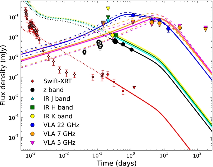
Figure 23. Same as Figure 17, with an additional reverse shock component to account for the mm detections at 0.4 and 1.3 d. The combined RS + FS model over-predicts the NIR K-band data between 0.01 and 0.05 d. See Appendix D for details.
Download figure:
Standard image High-resolution image
In summary, a combined RS + FS model with Γ ∼ 500 can explain the significant excess flux density in the millimeter. The model overpredicts the NIR K-band observations at 0.01 to 0.05 d, which could potentially be explained by a lower contribution from the FS than expected, due to energy injection over this period.
Footnotes
- 7
- 8
IRAF is distributed by the National Optical Astronomy Observatory, which is operated by the Association of Universities for Research in Astronomy (AURA) under cooperative agreement with the National Science Foundation.
- 9
All magnitudes are in the AB system and not corrected for Galactic extinction, unless otherwise mentioned.
- 10
We impose a floor of 5% on the uncertainty of each data point, as explained in Section 4.
- 11
Credible intervals are summary statistics for posterior density functions and are Bayesian analogues to the "confidence intervals" used in frequentist statistics. In this article, we use credible intervals based on percentiles of the posterior density, defined such that the probability of the parameter lying below and above the interval are equal. Such an interval includes the median of the posterior density by construction.
- 12
We set s = 5 for the jet break (Granot et al. 2001), the precise value having negligible impact on derived physical parameters.
- 13
Wherever light curves do not show any signature of flattening at late times, or when the last data point in a light curve is a deep non-detection, we assume the host flux is negligible and set it to zero to avoid biasing the model.
- 14
When plotting histograms of the logarithm of a quantity, we transform the width of the bins appropriately such that the height of the bin is equal to the value of the posterior density.
- 15
The uncertainty on the median is computed using Greenwood's formula for the variance of the Kaplan–Meier estimate of the cumulative distribution function. This method accounts for both upper and lower limits, which exist in the data.
- 16