


ABSTRACT
We present a combined X-ray, optical, and radio analysis of the galaxy group IC 1860 using the currently available Chandra and XMM data, multi-object spectroscopy data from the literature, and Giant Metrewave Radio Telescope (GMRT) data. The Chandra and XMM imaging and spectroscopy reveal two surface brightness discontinuities at 45 and 76 kpc shown to be consistent with a pair of cold fronts. These features are interpreted as due to sloshing of the central gas induced by an off-axis minor merger with a perturber. This scenario is further supported by the presence of a peculiar velocity of the central galaxy IC 1860 and the identification of a possible perturber in the optically disturbed spiral galaxy IC 1859. The identification of the perturber is consistent with the comparison with numerical simulations of sloshing. The GMRT observation at 325 MHz shows faint, extended radio emission contained within the inner cold front, as seen in some galaxy clusters hosting diffuse radio mini-halos. However, unlike mini-halos, no particle reacceleration is needed to explain the extended radio emission, which is consistent with aged radio plasma redistributed by the sloshing. There is a strong analogy between the X-ray and optical phenomenology of the IC 1860 group and that of two other groups, NGC 5044 and NGC 5846, showing cold fronts. The evidence presented in this paper is among the strongest supporting the currently favored model of cold-front formation in relaxed objects and establishes the group scale as a chief environment for studying this phenomenon.
1. INTRODUCTION
The current generation of X-ray telescopes (XMM and, to a greater degree, Chandra) with their angular resolution and sensitivity has revealed a wealth of small scale features in the intra-cluster medium (ICM) and intra-group medium. One particularly interesting feature is the phenomenon of "cold fronts," i.e., sharp surface brightness discontinuities, interpreted as contact edges between regions of gas with different entropies (see the review by Markevitch & Vikhlinin 2007). Cold fronts appear to be almost ubiquitous in galaxy clusters (Markevitch et al. 2003; Ghizzardi et al. 2010; Laganá et al. 2010) and they are found both in dynamically active objects and in cool core relaxed clusters. In merging clusters, cold fronts arise during merger events through ram-pressure stripping mechanisms that induce discontinuity among the merging dense subcluster and the less dense surrounding ICM (e.g., Vikhlinin et al. 2001). In relaxed clusters, cold fronts are most likely induced by minor mergers that produce a disturbance on the gas in the core of the main cluster, displace it from the center of the potential well, and decouple it from the underlying dark matter halo through ram pressure (Markevitch et al. 2001; Churazov et al. 2003; Ascasibar & Markevitch 2006). The oscillation of the gas of the core around the minimum of the potential generates a succession of radially propagating cold fronts, appearing as concentric edges in the surface brightness distribution of the cluster. These fronts may form a spiral structure when the sloshing direction is near the plane of the sky. When the sloshing direction is not in the plane of the sky, concentric arcs are observed. The sequence of events is described in great detail in the simulations presented in Ascasibar & Markevitch (2006).
Cold fronts are unique tools for understanding the physical properties of the ICM (e.g., Markevitch & Vikhlinin 2007). They can also be used in principle as a gauge of the merger activity (Owers et al. 2009a), in particular of the more frequent minor merging of smaller subsystems compared to the less frequent and more spectacular major mergers. Cold fronts do not need a favorable geometry for being detected like the more elusive shock fronts (e.g., Markevitch 2010) and they may provide the only indication at X-ray wavelengths of a minor merger in a seemingly relaxed cluster. Cold fronts can be used, with the help of simulations, to infer many merger characteristics, such as the presence and size of a spiral pattern in the surface brightness distribution being inferred from the direction and time of peri-center passage of the perturber (Ascasibar & Markevitch 2006; Johnson et al. 2010; Roediger et al. 2011).
Recently, gas sloshing in the core has also been invoked to explain the formation of diffuse radio minihalos in relaxed, cool-core clusters. These faint, steep-spectrum radio sources are relatively rare, with only a few clusters with confirmed detections (Feretti et al. 2012). A spatial correlation between the minihalo emission and cold fronts has been observed in a few clusters (Mazzotta & Giacintucci 2008; S. Giacintucci et al., in preparation), with the minihalos contained within the region confined by the cold fronts, suggesting a tight connection between sloshing motions and the origin of minihalos. Recently, ZuHone et al. (2013) showed with high resolution MHD simulations that gas sloshing can lead to turbulent reacceleration of relativistic electron seeds (e.g., from past active galactic nucleus (AGN) activity) and can produce diffuse radio emission within the envelope of the sloshing cold fronts.
Another complementary path to the study of the presence and dynamics of cluster mergers uses optical data to perform a spatial and kinematical analysis of member galaxies. These types of studies allow us to reveal and measure the amount of substructure, and to detect and analyze possible pre-merging clumps or merger remnants (e.g., Girardi & Biviano 2002). This is certainly interesting for major merger clusters which are very rich in optical substructures (see, for example, the DARC—Dynamical Analysis of Radio Clusters—project; Girardi et al. 2007) but even more so in the case of the minor merger scenario for sloshing. The assumption of a single Gaussian distribution is a good description for the galaxy velocities of the main cluster and the recently merged perturber may be identified by means of an optical/dynamical substructure search (e.g., Owers et al. 2011a). Optical studies can also investigate the presence of peculiar velocities of the bright central galaxy (BCG). One of the observable effects of the merger scenario discussed by Ascasibar & Markevitch (2006) is the fact that, if the BCG sits at the peak of the dark matter distribution, it is expected to start oscillating along with it after each subcluster flyby. Gas sloshing and BCG peculiar velocities are caused by the same minor mergers. Given the increasing number of objects showing sloshing cold fronts, this can also explain the large and apparently puzzling number of systems showing peculiar velocities of their BCGs (e.g., van den Bosch et al. 2005; Coziol et al. 2009). As a matter of fact, Miralda-Escude (1995, p. 515) looking at the early evidence of BCGs spatially coincident with the centers of dark matter halos producing lensing features, commented that "the fact that cD galaxies often have large peculiar velocities relative to the average of the cluster galaxies has been used as an argument against their identification as cluster centers: however, clusters are continuously merging, and their density peaks do not need to coincide with their centers of mass. Substructure will cause the density peaks to move, in response to the gravitational forces of the in-falling material."
The fact that sloshing cold fronts have also been detected at the smaller mass scales of poor clusters (e.g., Virgo; Simionescu et al. 2010) and of groups of galaxies (Gastaldello et al. 2009; Randall et al. 2009; Machacek et al. 2011) is yet another manifestation of the hierarchical nature of structure formation. At this mass scale even a single massive galaxy can be the responsible perturber and the X-ray signature of the sloshing cold front is a signature of the gravitational interaction between the galaxy (and its halo) and its host group.
The aim of this paper is to investigate sloshing features, such as cold fronts and spirals in the surface brightness distribution, in the nearby, X-ray-bright galaxy group IC 1860. We will look for other observable properties of the sloshing scenario such as a peculiar velocity of the BCG and extended radio emission possibly related to the presence of sloshing. We present in detail the results of the available XMM and Chandra data of the object, the available optical data in the literature, and new Giant Metrewave Radio Telescope (GMRT) data. We will then compare the observed features in IC 1860 with two other groups hosting cold fronts, NGC 5044 and NGC 5846.
The group IC 1860 was originally classified as a Dressler cluster (DC-0247-31; Dressler 1980) and it is also known as AS301 (Abell et al. 1989). It appears in many other catalogs, in particular the catalog of Maia et al. (1989). It is a nearby group of galaxies at z = 0.022 (at a distance of 97 Mpc with the cosmology adopted in this paper) and its optical structure/membership has been studied in Dressler & Shectman (1988) and, in particular, given the many additional redshifts provided by the 2dF redshift survey, by Burgett et al. (2004). It has been discovered in the X-ray band by the Einstein X-Ray Observatory (Burstein et al. 1997) and ROSAT showed the presence of extended and diffuse group X-ray emission at a temperature of ∼1 keV (Mulchaey et al. 2003). Chandra imaging showed no evidence of AGN-induced activity in the form of cavities in the core (Dunn et al. 2010). In our previous XMM analysis (Gastaldello et al. 2007) we mainly focused on the azimuthally averaged radial properties of the system for the purpose of mass analysis, however, noticing the presence of a possible disturbance in the surface brightness distribution.
The paper is organized as follows: in Section 2 we summarize the XMM and Chandra data reduction and analysis; in Section 3 we analyze the X-ray images and surface brightness profiles finding evidence of a set of two surface brightness discontinuities and an excess brightness spiral feature; in Section 4 we perform a spectral analysis of the temperature structure of the group finding evidence that the surface brightness discontinuities are cold fronts; in Section 5 we model the pressure jumps between the cold fronts and in Section 6 we discuss the possible systematics of our X-ray analysis; in Section 7 and in Section 8 we present the analysis of the available optical and GMRT data, respectively. In Section 9 we use simulations to constrain the merger geometry of IC 1860 and in Section 10 we discuss our results, making comparisons with the groups NGC 5044 and NGC 5846. Additional analysis performed on these groups is presented in Appendix A; in Section 11 we summarize our results. We also report on the narrow angle tail radio galaxy IC 1858 in Appendix C.
The cosmology adopted in this paper assumes a flat universe with H0 = 70 km s−1 Mpc−1, Ωm = 0.3, and ΩΛ = 0.7. All the errors quoted are at the 68% confidence limit. At the distance of IC 1860, 1' corresponds to 26.7 kpc.
2. OBSERVATIONS AND DATA PREPARATION
IC 1860 has been observed by XMM on 2003 February 4 (ObsID 0146510401) with the EPIC MOS and pn cameras for 39 and 38 ks respectively and by Chandra with the ACIS-S configuration on 2009 September (ObsID 10537) for 40 ks. We used both Chandra and XMM available archival data and we took advantage of the different characteristic of the two satellites. We exploited the wider field of view provided by XMM to analyze the source structure at larger radii while the higher resolution of Chandra allowed us to explore the details of the source in the inner region. We processed the data following the standard SAS15 and CIAO16 threads; in the following subsections we briefly describe the data preparation.
2.1. XMM
Starting from the Observation Data Files retrieved from the XMM-Newton archive, we generated calibrated event files with SAS, version 11.0, using the tasks emchain and epchain. We removed proton flares both from the hard and the soft light curve, using respectively a fixed threshold criterion and a σ-clipping technique, as described in Rossetti & Molendi (2010). We also checked for residual contamination by a quiescent soft-proton component, evaluating the in-over-out ratio as defined in De Luca & Molendi (2004). Net exposure time after proton flare correction is 34.5 ks for MOS-1, 34.8 ks for MOS-2, and 29.4 ks for pn. We checked the observation for contamination by solar wind charge exchange: the Advanced Composition Explorer (ACE) SWEPAM17 proton flux was less than 4 × 10⁸ protons s−1 cm−2 and the SWICS O+7/O+6 ratio was less than 0.3, values which are typical of the quiescent Sun (Snowden et al. 2004). The spectra of the out-of-field-of-view events of CCD 4 of MOS1 showed an anomalously high flux in the soft band (see Kuntz & Snowden 2008) and it was therefore excluded from our analysis.
We then filtered the events according to standard pattern and flag criteria and we performed out-of-time correction for pn. For each detector we created images in the 0.5–2 keV band and exposure maps. We detected point sources using the task ewavelet and masked them using a circular region centered at the source position and with a 25'' radius. Using the task emosaic, we combined the MOS images into a single exposure-corrected image shown Figure 1 and discussed in Section 3.1.

Figure 1. Exposure-corrected mosaic of the XMM MOS1 and MOS2 images Gaussian-smoothed on a 3'' scale. Superposed over the image are the angular sectors used for the surface brightness profiles of Figure 2 and discussed in the text.
Download figure:
Standard image High-resolution image2.2. Chandra
In order to ensure the most up-to-date calibration, we reprocessed all Chandra data starting from level 1 event files, using the X-ray analysis package CIAO 4.3 in conjunction with the Chandra calibration database (Caldb) version 4.1.3. We took into account time-dependent drift in the detector gain and charge transfer inefficiency as implemented in the CIAO tools. To clean the data from periods of enhanced background, we performed a σ-clipping to the light curve in the 0.5–7 keV band. The final exposure time after deflaring is 35.7 ks. Point sources were detected with the CIAO tool wavdetect and then excluded from all the following steps of the data analysis using an appropriate mask region. We used the blank-sky data set provided in the CALDB to perform background analysis, after properly re-processing and re-projecting it. To take into account possible temporal variations of instrumental background, we rescaled the background file for the ratio between the count-rate of the observation and the background. To calculate the proper rescaling factor, we extracted spectra for both background and source files from an external region not contaminated by source emission and we quantified the count-rate ratio in the hard band 9–12 keV. We then generated an image the 0.7–2.0 keV band and corrected it for its exposure map. The analysis we performed on the Chandra image is discussed in Section 3.2.
3. X-RAY IMAGES AND SURFACE BRIGHTNESS PROFILES
The sloshing scenario has been introduced to explain a number of features present in the surface brightness distribution of relaxed clusters and groups, in particular the presence of concentric sharp surface brightness edges which have a temperature jump consistent with being cold fronts and the presence of an excess corresponding to spiral- or arc-shaped brighter regions inside the actual fronts. The morphology depends mainly on the angle between our line-of-sight (LOS) and the orbital plane of the subcluster: a spiral-like structure is seen if the interaction is seen face-on; if, by contrast, the LOS is parallel to the orbital plane, arcs are seen on alternating sides of the cluster core (Ascasibar & Markevitch 2006; Roediger et al. 2011). In the following sections we will investigate the surface brightness distribution of the X-ray emission of IC 1860 as revealed by the XMM and Chandra data to look for such features.
3.1. The Outer Surface Brightness Edge
Visual inspection of the mosaic image of the two MOS cameras (Figure 1) clearly reveals the presence of a sharp brightness discontinuity in the northwest direction (P.A. 250°–340°, position angles measured from the N direction). In the opposite direction (P.A. 70°–160°), at large radii the group is more elongated and in the inner region a luminous plume is seen; this feature is sharper in the Chandra image so we will focus on it in Section 3.2. To confirm this qualitative impression, we compared the surface brightness profiles in four angular sectors 90° wide as depicted in Figure 1. An evident slope change is seen in the 250°–340° profile, at a radius of ∼170'' (Figure 2); conversely, the profiles of the other three control sectors are fairly smooth with a continuous derivative. In the right panel of Figure 2 we provide a zoom over the interesting radial region where the edge is seen. The feature is also detected in the pn and the ACIS data (Figure 3), however, it is less evident in the Chandra image, being close to the outer edge of the CCD.

Figure 2. Left panel: XMM surface brightness profiles in the selected angular sectors discussed in the text (Section 3.1) and shown in Figure 1. Green circles: sector P.A. 340°–70°. Blue circles: sector P.A. 70°–160°. Black circles: sector P.A. 160°–250°. Red circles: sector P.A. 250°–340°. The outer edge can be easily seen in the sector P.A. 250°–340°. Right panel: zoom over the interesting radial region for the outer edge. The slope of the source profile is steeper in the sector P.A. 250°–340° than in the control sector P.A. 340°–70°.
Download figure:
Standard image High-resolution image
Figure 3. Chandra 0.7–2.0 keV image Gaussian smoothed on a 3'' scale and corrected for exposure map. Superposed over the image are the angular sectors used for the surface brightness profiles of Figure 4 and discussed in the text.
Download figure:
Standard image High-resolution image3.2. The Inner Surface Brightness Edge
The Chandra image of Figure 3 provides more detailed insight into the inner region of IC 1860, confirming what we have already pointed out in Section 3.1: in a narrow sector at P.A. 130°–160° the source is elongated in a luminous tail ending in a surface brightness edge. In Figure 4 we compare the profile of the source in this sector with the profile of the source in two other control sectors as depicted in Figure 4. The profile of the source in the sector at P.A. 130°–160° is clearly different with respect to the other control profiles in the radial range 20''–100''; the feature is more evident in the zoom of the left panel of Figure 4: a peak corresponding to the luminous tail is seen, then at a radius of ∼100'', the profile flattens out. The feature is also clearly seen in the XMM data.

Figure 4. Left panel: Chandra surface brightness profiles in the selected angular sectors discussed in the text (Section 3.2) and shown in Figure 3. Black circles: sector P.A. 340°–130°. Red circles: sector P.A. 130°–160°. Green circles: sector P.A. 160°–250°. Blue circles: sector 250°–340°. The inner edge and enhancement of the surface brightness profile are evident in the sector P.A. 130°–160°. A steepening of the sector P.A. 250°–340° profile can also be seen at the edge of Chandra field of view, consistent with the XMM feature of Figure 2. Right panel: zoom over the interesting radial region for the inner edge. The slope of the source profile is rapidly changing in the sector P.A. 130°–160° than in the control sector P.A. 340°–130°.
Download figure:
Standard image High-resolution image3.3. The Spiral Feature
In Figure 5 we present the surface brightness residual map between the XMM data and the best-fit radially symmetric two-dimensional β-model describing the surface brightness distribution obtained with Sherpa: the residual map highlights the appearance of sloshing features. A characteristic spiral pattern in surface brightness can be seen, with the tail being confined by the outer cold front. The qualitative impression is that the overall morphology is tilted with respect to the plane of the sky, with the mushroom structure formed by the coolest gas and seen in many hydrodynamic simulations (e.g., the snapshot at 1.9 Gyr of Figure 7 of Ascasibar & Markevitch 2006) seen almost face on. The southern edge of this "mushroom head" coincides with the inner surface brightness discontinuity.
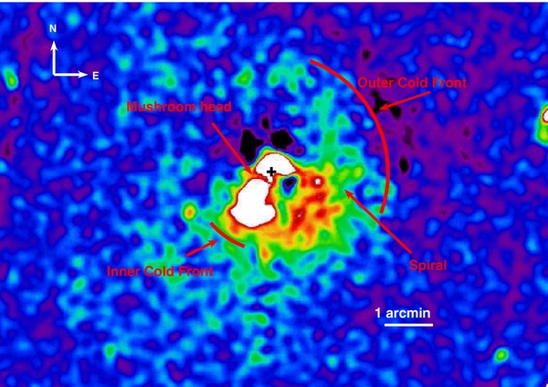
Figure 5. XMM residual map, obtained by subtracting to the image of Figure 1 the best fit beta model for the data. The center of IC 1860 is shown by the black cross and the position and extent of the surface brightness edges by the red arcs. The "mushroom head" discussed in the text is the central region with white color. The image has been processed to remove point sources.
Download figure:
Standard image High-resolution image4. X-RAY SPECTRAL ANALYSIS
To further investigate the nature of the brightness discontinuities we analyzed the temperature profiles across them. For this purpose we extracted XMM and Chandra spectra in several radial bins,18 along the angular sectors containing the edges (P.A. 250°–340° and P.A. 130°–160°) and in two other control sectors (P.A. 340°–70°; P.A. 160°–250°) in order to measure the temperature trend across the edges and check if it is actually different from the overall undisturbed temperature profile.
We extracted XMM spectra generating a response file and an ancillary response file using the standard SAS tasks rmfgen and arfgen in extended source mode; we extracted Chandra spectra generating count-weighted spectral response matrices appropriate for each region using the task specextract. For each region, we also extracted background spectra from the blank-field event files. All spectra were re-binned to ensure a minimum 20 counts bin−1 and fitted in the 0.5–5.0 keV band, with an APEC (Smith et al. 2001) plasma model as implemented in Xspec version 11.0. We take into account galactic absorption using a phabs model with the hydrogen column density frozen to the value provided in Kalberla et al. (2005). In Section 6 we will explore the sensitivity of the results to the above assumptions.
In Table 1 we present the results of the spectral fits in the interesting radial bins inside and outside the edges and in the same radial bins in the control sectors. In Figure 6 we show the temperature profile along the sectors containing the edges as obtained with XMM (left panel) and Chandra (right panel): the vertical dashed lines mark the radius of the two brightness discontinuities. The region outside the outer edge is covered only by the larger XMM field of view; therefore the complete temperature profile along the outer edge is available only in the left panel of Figure 6.

Figure 6. Left panel: XMM temperature profile along the sectors containing the surface brightness edge. Blue points: outer edge sector, P.A. 250°–340°. Red points: inner edge sector, P.A. 130°–160°. Horizontal error bars marks the radial extensions of the bins we used for the spectral analysis. The vertical dashed lines mark the radial position of inner and outer surface brightness edges. Right panel: Chandra temperature profile along the sectors containing the surface brightness edge. Green points: outer edge sector, P.A. 250°–340°. Magenta points: inner edge sector, P.A. 130°–160°. Horizontal error bars marks the radial extensions of the bin for the spectral analysis. The vertical dashed lines marks the radial position of the surface brightness edge as in the left panel: note that the more external radial bin of the XMM temperature profile falls outside Chandra field of view and for clarity of the plot the temperature axes do not have the same extent in the two profiles.
Download figure:
Standard image High-resolution imageTable 1. Parameters from the Spectral Fits across the Edges
| Radii P.A. | XMM | Chandra | ||||
|---|---|---|---|---|---|---|
| T | ZFe | T | ZFe | |||
| χ2/dof | (keV) | Solar | χ2/dof | (keV) | Solar | |
| Outer edge | ||||||
| 100''–150'' 250°–340° | 98/105 | 64/70 | ||||
| 180''–230'' 250°–340° | 55/68 | ... | ... | ... | ||
| Control regions | ||||||
| 100''–150'' 340°–70° | 84/122 | 58/66 | ||||
| 180''–230'' 340°–70° | 73/91 | ... | ... | ... | ||
| 100''–150'' 160°–250° | 139/150 | 72/72 | ||||
| 180''–230'' 160°–250° | 94/113 | ... | ... | ... | ||
| Inner edge | ||||||
| 60''–90'' 130°–160° | 48/54 | 24/21 | ||||
| 100''–150'' 130°–160°a | 29/50 | 39/47 | ||||
| Control regions | ||||||
| 60''–90'' 340°–70° | 63/81 | 29/41 | ||||
| 100''–150'' 340°–70° | 84/122 | 58/66 | ||||
| 60''–90'' 160°–250° | 126/123 | 60/55 | ||||
| 100''–150'' 160°–250° | 139/150 | 72/72 | ||||


Notes. Results of XMM and Chandra spectral fits, in the radial bins inside and outside the surface brightness edges, as discussed in Section 4. The first and the second columns refers to the radial and angular range of each bins. XMM and Chandra are reported as labeled on the top of the table. No entry in the Chandra rows means that the referred bins falls out the available field of view. aThe Chandra data have been extracted in a 100°–160° P.A. region to increase the statistics.
Download table as: ASCIITypeset image
For the inner edge both XMM and Chandra temperature profiles show an enhancement of the gas temperature across the discontinuity; the same behavior is not observed in the control sectors. It is also clear that as expected there is asymmetry in the temperature profile, in particular the part of the "mushroom head" of emission in the SE leading to the inner edge is cooler than the surroundings. The temperature trend observed by the two instruments is the same, although in the outer radial bin the Chandra temperature is 38% higher than the XMM one. We interpreted this discrepancy as due to a temperature mixing in the XMM spectrum, induced by its larger point-spread function (PSF). To check this hypothesis we compared XMM and Chandra temperatures in two wider (P.A: 100°–1600°) radial bins at the same radii where we observed the temperature discrepancy (100''–150'') and further away (150''–210''). With the given interpretation, away from the disturbed region where the edge is seen, the discrepancy between Chandra and XMM temperatures falls to the 12% level.
There is no statistically significant change in the temperature across the outer edge. The quality of the data allows us only to measure projected temperatures meaning that the true de-projected difference of temperatures across the front can be lower. Furthermore, when contrasted with the declining trend of the control regions at different azimuthal angles, the picture is consistent with cooler gas inside the edge. Similar behavior has been seen for the outer edge in the NGC 5044 (Gastaldello et al. 2009) and NGC 5846 (Machacek et al. 2011) groups.
5. FITS OF THE SURFACE BRIGHTNESS EDGES
In order to characterize in a quantitative way the density jump across the cold front we modeled the surface brightness profile across the discontinuity following the approach of Rossetti et al. (2007) and Gastaldello et al. (2010). We assume that the gas density profile is described by a power law on either side of the edge,

where rcf is the cold front radius and we derive the parameters of this model from the fit of the projected surface brightness profile, which can be expressed as the integral of the emissivity along the LOS:

where K is a constant and we took into account the dependence of the emissivity of the temperature T and metal abundance Z.
We fit the outer part of the surface brightness profile to set the external component parameters and we successively derive the best fit parameters of the innermost part. We applied this method to the XMM profile across the outer edge and to the Chandra profile across the inner edge. Our results are summarized in Table 2 and in Figure 7 we plot the surface brightness profile and the best fit model respectively for the outer (left panel) and inner edges (right panel).

Figure 7. Left panel: fit of the XMM surface brightness profile along the outer edge. The superposed solid line represents the best fit two power law model, as discussed in Section 5. Right panel: fit of the Chandra surface brightness profile along the outer edge. The superposed solid line represents the best fit two power law model. Note that, as discussed in Section 5, the model does not fit the profile in the radial range ∼20''–∼50'', where the source is elongated in a narrow luminous tail.
Download figure:
Standard image High-resolution imageTable 2. Parameters from the Fits of the Surface Brightness Profiles across the Edges
| r (kpc) | γin | γout | M | |||
|---|---|---|---|---|---|---|
| Outer edge P.A. 130°–160° | 76 | 0.88 ± 0.09 | 0.85 ± 0.03 | 1.28 ± 0.03 | 1.27 ± 0.10 | 0.55 ± 0.08 |
| Inner edge P.A. 250°–340° | 45 | 0.90 ± 0.05 | 1.00 ± 0.06 | 1.65 ± 0.06 | 1.30 ± 0.13 |


Notes. Results from the XMM and Chandra profiles fits, along the outer and the inner edges respectively. The first two columns refer to the internal and external power-law indices, as discussed in the text, Section 5. We then report the derived density and pressure jumps and the Mach number M.
Download table as: ASCIITypeset image
For the outer edge the agreement between the chosen model and the data is good. We find a density jump of nin/nout = 1.28 ± 0.03 that, when combined with the temperature and abundance information in the regions inside and outside the front reported in Table 1, gives a pressure ratio of Pin/Pout = 1.27 ± 0.10. If this pressure ratio is interpreted as evidence for bulk motion of the cold front then following Vikhlinin et al. (2001) we infer that the front is moving subsonically with a Mach number M = 0.55 ± 0.08.
In the profile of the inner edge a surface brightness bump is seen between ∼20'' and ∼50'', which is not well fitted by the adopted double power law model. This discrepancy was expected, given the peculiar shape of the source in the sector containing the edge; the observed bump corresponds roughly to the region where the source is elongated in a narrow luminous tongue. Except for this peculiar structure, the profile inside and outside the edge is well described by the model and then internal and external power law indices are well determined. We find a density jump of nin/nout = 1.65 ± 0.06 and, using the Chandra temperature and abundance determination, the pressure ratio is Pin/Pout = 1.30 ± 0.13 corresponding to a Mach number . We will explore the robustness of this result with respect to various analysis choices in Section 6.5.

6. SYSTEMATIC ERRORS
In this section we provide an investigation of the possible systematic errors affecting the temperatures and abundances across the edges quoted in Table 1. Readers who are uninterested in these technical details can safely skip to the following section.
6.1. Plasma Codes
We compared the results obtained using the APEC code to those obtained using the MEKAL code (Kaastra & Mewe 1993). The different implementations of the atomic physics and different emission line lists in the plasma codes produce no qualitative differences between the fits and no significative variations of χ2. Variations of the fitted XMM temperatures are all within ∼5% and well within the statistical errors; all fitted XMM abundance agrees within ∼9%.
For the Chandra data the use of the different plasma code produces a 5% variation in the inner spectral temperature and a 4% variation in the outer one.
6.2. Bandwidth
We explored the sensitivity of our results to the default lower limit of the bandpass, keV. For comparison we performed spectral fits with keV and keV. The fitted temperatures are substantially unchanged and consistent within the statistical errors, both for XMM and for Chandra; an analogous result holds for the iron abundances.


6.3. Variable NH
To check for possible deviations of NH from the galactic value of Kalberla et al. (2005), we perform a spectral fit leaving NH as a free parameter. For the XMM spectra the fitted NH values are higher by a factor ∼3 with respect to the Galactic value; the correspondent variations of fitted temperatures are within ∼9%; absolute variations of temperatures and abundances are, however, well accounted for by the quoted statistical errors.
The parameters of the Chandra spectrum of the region inside the inner edge are basically unchanged and the fitted NH agrees with the Galactic value within 1σ. The spectral fits of the region outside the inner edge give instead a higher NH by a factor of ∼4; the corresponding fitted temperature (), however, agrees with the quoted one within the statistical errors and its lower limit is still consistent with an enhancement of the temperature outside the inner edge.

6.4. Background
To account for systematic errors in background normalization, we performed spectral fits allowing it to vary ±5%. Temperatures and abundances are insensitive to this variation in all the considered XMM spectra; variations of Chandra temperatures are all within 10%, while iron abundances are basically unchanged.
6.5. Cold Front Modeling
The inner cold front is not perfectly modeled by the expression given in Equation (1) and there are discrepancies between the spectral parameters at either side of the front between the Chandra and XMM values. We explore the sensitivity of the derived Mach number with respect to the choice of the fitting range of the surface brightness profiles and the adopted temperature and abundance values. The fiducial measurement is derived by using the Chandra spectral values and fitting the internal component in the range 7''–40''. If we fit the internal component in the range 7''–30'' we obtain a worse fit and a Mach number and if we use instead a 60''–90'' range to better model the excess, with the problem of deriving a very high density in the inner regions, we obtain a Mach number . Using the XMM spectral parameters instead of the Chandra values we obtain . We therefore conclude that our determination in Section 5 is rather robust to possible systematic errors.


7. OPTICAL ANALYSIS
In this section we present our optical analysis which includes the determination of group membership and substructure detection. The Digital Sky Survey (DSS) image of the central region of the group is shown in Figure 8. The purpose of the optical analysis is to search for substructures and to use them together with the X-ray observations to investigate the dynamical state of the IC 1860 group.

Figure 8. DSS image of the central region of the IC 1860 group. IC 1860, IC 1859, and ESO 416-G033 are indicated (see discussion in Section 7.3.3). IC 1858 is also indicated (see discussion in Appendix C). Red labels refer to galaxies rejected by the shifting gapper method (see Section 7.1), with numbers referring to the number entry in the catalog of Table 3.
Download figure:
Standard image High-resolution image7.1. Sample Selection and Group Membership
We used the NASA/IPAC Extragalactic Database (NED) to collect galaxies with known recession velocities within 60' (1.6 Mpc at the redshift of the source) of the optical position of the galaxy IC 1860 which coincides with the peak of the diffuse X-ray emission of the group. This corresponds to 1.7 times the virial radius (r100) estimated from hydrostatic mass analysis of the XMM data in Gastaldello et al. (2007); this is justified by the search for a possible perturber following the scenario of Ascasibar & Markevitch (2006). The primary sources of these velocities are: 2dFGRS (Colless et al. 2003), the redshift catalog of Dressler & Shectman (1988), the Southern Sky Redshift Survey (da Costa et al. 1998), the redshift survey using the ESO OPTOPUS multifiber instrument performed by Stein (1996), the 6dFGS (Jones et al. 2009), and the Durham/UKST (DUKST) redshift survey (Ratcliffe et al. 1998). Group members have been selected through the elimination of background and foreground galaxies along the LOS to IC1860. An initial rejection was performed using the "velocity gap" method outlined by De Propris et al. (2002) where the galaxies are sorted in redshift space and their velocity gap, defined for the nth galaxy as Δvn = czn + 1 − czn is calculated. Clusters and groups appear as well populated peaks in redshift space which are well separated by velocity gaps from the nearest foreground and background galaxies: we uses 1000 km s−1 as velocity gap and Figure 9 shows that this procedure clearly detects IC 1860 as a peak at z = 0.02 populated by 81 galaxies. This initial eighty-one-member list for the IC1860 group is shown in Table 3, based mainly on the homogeneous 2dF sample which consists of 74 objects. Additional objects come from the other catalogs and in Appendix B we checked the consistency of the various measurements.

Figure 9. Histogram of all the available redshifts in NED within a 60' field around IC 1860 (galaxies with z > 0.25 are not shown for display purposes). The IC1860 group stands out as the redshift peak at z = 0.02.
Download figure:
Standard image High-resolution imageTable 3. IC1860 Group Galaxies
| ID | Galaxy Identifier | R.A. | Decl. | cz | cz Error | Source |
|---|---|---|---|---|---|---|
| 1 | IC 1860 | 42.39047 | −31.1891 | 6866 | 20 | Stein (1996) |
| 2 | 2MASX J02493302-3111569 | 42.38674 | −31.19923 | 7532 | 33 | Stein (1996) |
| 3 | 2MASX J02493200-3110229 | 42.38304 | −31.17301 | 6865 | 64 | 2dF |
| 4 | 2dFGRS S394Z186 | 42.38183 | −31.16742 | 7525 | 89 | 2dF |
| 5 | 2MASX J02493933-3112169 | 42.41373 | −31.20474 | 7905 | 20 | Stein (1996) |
| 6* | 2MASX J02494174-3112139 | 42.42371 | −31.20347 | 8664 | 64 | 2dF |
| 7 | 2dFGRS S394Z183 | 42.4035 | −31.2205 | 6416 | 123 | 2dF |
| 8* | 2dFGRS S394Z176 | 42.4285 | −31.19736 | 8784 | 64 | 2dF |
| 9 | 2MASX J02492990-3109249 | 42.37436 | −31.15675 | 7945 | 64 | 2dF |
| 10 | MCG -05-07-036 | 42.34263 | −31.18172 | 6835 | 64 | 2dF |
| 11 | 2dFGRS S467Z174 | 42.43247 | −31.15795 | 6985 | 64 | 2dF |
| 12 | 2MASX J02493349-3107159 | 42.38908 | −31.12111 | 6985 | 64 | 2dF |
| 13 | 2dFGRS S467Z173 | 42.45072 | −31.13592 | 6835 | 64 | 2dF |
| 14 | 2MASXi J0249572-311036 | 42.4886 | −31.17639 | 6086 | 64 | 2dF |
| 15 | 2dFGRS S394Z181 | 42.398 | −31.09167 | 6266 | 64 | 2dF |
| 16 | 2MASX J02495627-3107599 | 42.48442 | −31.13339 | 7195 | 64 | 2dF |
| 17 | IC 1859 | 42.26635 | −31.17251 | 5966 | 64 | 2dF |
| 18 | 2dFGRS S467Z168 | 42.52021 | −31.13019 | 7664 | 64 | 2dF |
| 19 | 2MFGC 02270 | 42.48279 | −31.2875 | 6356 | 64 | 2dF |
| 20 | IC 1858 | 42.28504 | −31.28958 | 6056 | 89 | 2dF |
| 21 | 2dFGRS S394Z189 | 42.30958 | −31.06367 | 6446 | 89 | 2dF |
| 22 | LSBG F416-020 | 42.50358 | −31.30597 | 6835 | 89 | 2dF |
| 23 | 2MASX J02485680-3106431 | 42.23634 | −31.11194 | 6835 | 64 | 2dF |
| 24 | 2MASX J02491494-3103060 | 42.31196 | −31.05162 | 6760 | 23 | Stein (1996) |
| 25 | 2MASX J02493567-3101249 | 42.39858 | −31.02364 | 6955 | 64 | 2dF |
| 26 | 2dFGRS S394Z174 | 42.45371 | −31.03258 | 7345 | 123 | 2dF |
| 27 | 2dFGRS S467Z163 | 42.56 | −31.29644 | 7315 | 89 | 2dF |
| 28 | ESO 416- G 033 | 42.40642 | −30.99583 | 6595 | 123 | 2dF |
| 29 | 2dFGRS S466Z088 | 42.23542 | −31.38433 | 6685 | 89 | 2dF |
| 30 | 2dFGRS S394Z172 | 42.47059 | −30.95476 | 7045 | 64 | 2dF |
| 31 | 2dFGRS S394Z162 | 42.68179 | −31.04658 | 7045 | 123 | 2dF |
| 32 | ESO 416- G 035 | 42.63233 | −31.39464 | 6535 | 64 | 2dF |
| 33 | 2dFGRS S394Z161 | 42.68804 | −31.04619 | 6625 | 89 | 2dF |
| 34 | DUKST 416-040 | 42.1205 | −31.37789 | 6026 | 123 | 2dF |
| 35 | 2dFGRS S394Z115 | 42.22129 | −30.88644 | 6505 | 123 | 2dF |
| 36 | 2MASX J02511626-3119392 | 42.81783 | −31.32758 | 6559 | 45 | 6dF |
| 37* | ESO 416- G 025 | 42.16992 | −31.53622 | 4977 | 64 | 2dF |
| 38 | ESO 416- G 036 | 42.64808 | −31.52008 | 7015 | 64 | 2dF |
| 39 | 2MASX J02504193-3130145 | 42.67467 | −31.50403 | 7135 | 64 | 2dF |
| 40 | ESO 416- G 034 | 42.60833 | −31.55828 | 7045 | 64 | 2dF |
| 41 | ESO 416- G 027 | 42.23883 | −30.79289 | 6835 | 64 | 2dF |
| 42 | LCSB S0441P | 41.89725 | −31.10831 | 6925 | 64 | 2dF |
| 43 | 2dFGRS S467Z150 | 42.70867 | −31.53058 | 6026 | 89 | 2dF |
| 44 | 2dFGRS S467Z190 | 42.28596 | −31.68119 | 6745 | 89 | 2dF |
| 45* | 2dFGRS S466Z100 | 42.13721 | −31.64678 | 5516 | 89 | 2dF |
| 46 | 2dFGRS S394Z155 | 42.919 | −30.94231 | 6446 | 123 | 2dF |
| 47 | 2dFGRS S467Z121 | 42.9955 | −31.09386 | 6386 | 64 | 2dF |
| 48 | 2dFGRS S467Z134 | 42.9345 | −31.48431 | 6865 | 64 | 2dF |
| 49 | LCSB L0144P | 42.83546 | −30.78181 | 7010 | 31 | 6dF |
| 50 | 2MASX J02483150-3142206 | 42.13125 | −31.70575 | 6835 | 64 | 2dF |
| 51 | 2MASX J02493534-3145319 | 42.39725 | −31.75886 | 6955 | 89 | 2dF |
| 52 | ESO 416- G 021 | 41.78033 | −31.48347 | 7435 | 89 | 2dF |
| 53 | 2dFGRS S467Z114 | 43.11317 | −31.32844 | 6505 | 123 | 2dF |
| 54 | DUKST 416-030 | 43.07238 | −30.94333 | 6655 | 64 | 2dF |
| 55 | 2MASX J02483040-3147366 | 42.12675 | −31.79356 | 6356 | 64 | 2dF |
| 56 | 2dFGRS S466Z087 | 42.24479 | −31.83344 | 6955 | 89 | 2dF |
| 57 | 2dFGRS S466Z140 | 41.79083 | −31.60678 | 6595 | 89 | 2dF |
| 58 | 2MASXi J0250166-303222 | 42.5695 | −30.5395 | 7075 | 64 | 2dF |
| 59 | 2dFGRS S467Z135 | 42.91488 | −31.73853 | 6895 | 123 | 2dF |
| 60* | 2dFGRS S393Z037 | 41.68479 | −30.78836 | 4707 | 123 | 2dF |
| 61 | DUKST 416-043 | 41.63875 | −31.54614 | 7345 | 89 | 2dF |
| 62 | ESO 416- G 040 | 43.11304 | −30.77653 | 6775 | 89 | 2dF |
| 63 | 2dFGRS S467Z137 | 42.854 | −31.82 | 6775 | 89 | 2dF |
| 64 | 2dFGRS S394Z041 | 42.92617 | −30.5975 | 6745 | 89 | 2dF |
| 65 | 2dFGRS S466Z101 | 42.14604 | −31.91153 | 6865 | 89 | 2dF |
| 66 | LCSB S0440P | 41.86242 | −31.81589 | 6838 | 150 | DUKST |
| 67 | AM 0250-310 | 43.22633 | −30.85742 | 6745 | 64 | 2dF |
| 68* | 2dFGRS S393Z025 | 41.89079 | −30.50036 | 5216 | 89 | 2dF |
| 69 | 2dFGRS S395Z027 | 43.00417 | −30.56647 | 6955 | 89 | 2dF |
| 70 | 2dFGRS S467Z136 | 42.87258 | −31.92583 | 6146 | 123 | 2dF |
| 71 | 2dFGRS S395Z037 | 43.33496 | −30.91456 | 6715 | 89 | 2dF |
| 72 | ESO 416-G 039 | 43.09304 | −31.81728 | 6625 | 64 | 2dF |
| 73 | 2dFGRS S394Z015 | 43.28067 | −30.77533 | 6416 | 64 | 2dF |
| 74 | 2dFGRS S393Z030 | 41.80092 | −30.47836 | 6805 | 89 | 2dF |
| 75 | 2dFGRS S395Z035 | 43.41779 | −31.16642 | 6386 | 64 | 2dF |
| 76 | ESO 416-G 041 | 43.37237 | −30.86036 | 6416 | 64 | 2dF |
| 77* | 2dFGRS S466Z122 | 41.98921 | −32.05119 | 4947 | 64 | 2dF |
| 78 | LSBG F416-018 | 43.264 | −31.75997 | 6296 | 123 | 2dF |
| 79 | 2dFGRS S466Z183 | 41.43917 | −31.69525 | 6595 | 89 | 2dF |
| 80 | 2dFGRS S466Z167 | 41.55225 | −31.85869 | 6446 | 123 | 2dF |
| 81 | 2dFGRS S466Z166 | 41.55658 | −31.88614 | 6985 | 89 | 2dF |
Notes. Columns are as follows: (1) galaxy identifier (2) right ascension (J2000), (3) declination (J2000), (4) recession velocity, (5) error on the recession velocity, (6) source of the measurement. The galaxies with entries in italics and marked with an asterisk are the galaxies rejected from membership by the shifting gapper method.
As a further refinement of the membership allocation process we used the slightly modified version of the "shifting gapper," first employed by Fadda et al. (1996), as described by Owers et al. (2009b). The method utilizes both radial and peculiar velocity information to separate interlopers from members as a function of groupcentric radius. The data are binned radially such that each bin contains at least 20 objects. Within each bin galaxies are sorted by peculiar velocity with velocity gaps determined in the peculiar velocity. Peculiar velocities were determined by estimating the mean group velocity using the biweight location estimator (Beers et al. 1990) which was assumed to represent the cosmological redshift of the group, zcos. The peculiar redshift of the galaxy is zpec = (zgal − zcos)/(1 + zcos) and the peculiar velocity is derived using the special relativistic formula vpec = c((1 + zpec)2 − 1)/((1 + zpec)2 + 1), where c is the speed of light. The "f pseudosigma" (Beers et al. 1990) derived from the first and third quartiles of the peculiar velocity distribution was used as the fixed gap to separate the group from the interlopers because of its robustness to the presence of interlopers. The above procedure was iterated until the number of members was stable. The results are shown in Figure 10 and the rejected galaxies are highlighted in Table 3.

Figure 10. Peculiar velocities as a function of the distance from the center of the IC 1860 group, illustrating the procedure of refinement of the membership using the shifting gapper technique (see text). The black circles represent galaxies allocated as group members while the red triangles are rejected foreground and background galaxies lying close to the group in redshift space.
Download figure:
Standard image High-resolution imageThe final group sample contains 74 members. The value for the biweight location estimator of the mean group velocity is 6753 ± 44 km s−1 which corresponds to zcos = 0.02252 ± 0.00015. We used the biweight scale estimator to estimate a velocity dispersion of 401 ± 46 km s−1. The errors for the redshift and velocity dispersion are 1σ and are estimated using the jackknife resampling technique.
In Figure 11 we show the velocity dispersion profile derived for the data. Bins contain 10 galaxies each and velocity dispersions have been calculated using the gapper algorithm (Beers et al. 1990). The profile shows the typical falling behavior with the radius expected for a relaxed object.

Figure 11. Velocity dispersion profile of the IC 1860 group, where IC 1860 is assumed to be the center of the group. Bins contain 10 galaxies each and 1σ jackknife errors are shown.
Download figure:
Standard image High-resolution image7.2. Peculiar Velocity of the Central Galaxy
We calculated the peculiar velocity of the central galaxy IC 1860 which is 113 ± 50 km s−1, just adding in quadrature the errors on the galaxy and group velocities. An offset velocity must lie outside a range defined by the cluster velocity dispersion to be significant (Gebhardt & Beers 1991). We therefore calculated the Z-score for the central galaxy (Equation (7) of Gebhardt & Beers 1991) which is 0.279 and its 90% confidence limits are (0.036, 0.520). The confidence interval has been calculated using 10,000 bootstrap resamplings and allowing for the measurement error of the central galaxy velocity by sampling from a Gaussian distribution with standard deviation set to the reported error as part of the bootstrap. The velocity offset is marginally significant at the 2.3σ level.
7.3. Substructure Detection
Given the presence of sloshing cold fronts in the X-ray-emitting medium of the IC 1860 group it is relevant to look for the presence of substructure and to possibly identify the merging sub-halo responsible for the onset of sloshing.
In general the higher the dimensionality of the substructure test, the more sensitive it is to substructure; however, the sensitivity of individual diagnostics depends on the LOS relative to the merger axis and therefore no single substructure test is the most sensitive in all situations; it is essential to apply a full range of statistical tests (e.g., Pinkney et al. 1996). In this section we apply a battery of statistical methods to the detection of substructure in IC 1860.
7.3.1. One-dimensional Tests for Substructure
We analyze the velocity distribution to look for departures from Gaussianity which can be attributed to dynamical activity. As a first test of Gaussianity, following Hou et al. (2009), we applied the Anderson–Darling (AD) test as the more reliable and powerful test at detecting real departures from an underlying Gaussian distribution. We used the AD test as implemented in the task ad.test of the package nortest in version 2.10 of the R statistical software environment19 (R Development Core Team 2011). When applied to the final group sample of 74 objects (the galaxies not highlighted in Table 3) the AD test returns a A2 statistic (following the notation of Hou et al. 2009, just A in the ad.test documentation) of 0.6146 which corresponds to a p value of 0.1059 (computed using the modified statistic A2*), therefore consistent with having a Gaussian distribution.
We estimated three shape indicators: the skewness, the kurtosis, and the scaled tail index, a robust indicator (Bird & Beers 1993). The values for the sample are 0.429 and 0.386 for skewness and kurtosis respectively and they show no departure from a Gaussian distribution (see Table 2 of Bird & Beers 1993 for 75 data points). The scaled tail index is 1.14, again consistent with a Gaussian distribution.
We investigated the presence of significant gaps in the velocity distribution following the weighted gap analysis of Beers et al. (1991) looking for normalized gaps larger than 2.25 since in random draws of a Gaussian distribution they arise at most in about 3% of the cases, independent of the sample size. We did not find any significant gap in the sample.
To detect subsets in the velocity distribution we also applied to the data Kaye's mixture model (KMM) test (Ashman et al. 1994). The KMM algorithm fits a user-specified number of Gaussian distributions to a data set and assesses the improvement of that fit over a single Gaussian. In addition, it provides an assignment of objects into groups. The KMM test is more appropriate in situations where theoretical and empirical arguments indicate that a Gaussian model is reasonable, such as for the LOS velocities in a dynamically relaxed cluster. Again, we did not find any significant partition of the sample.
To summarize the results of the one-dimensional (1D) tests, we found no evidence of substructure in the velocity distribution in the final group sample. Note that the same battery of tests applied to the unrefined sample would detect a significant departure from the Gaussianity. Thus, the shifting gapper refinement of the membership allocation has been effective in removing small foreground and background groups; in particular the central group of high velocity interlopers was already noticed by Burgett et al. (2004).
7.3.2. Three-dimensional Tests for Substructure
The existence of correlations between positions and velocities of cluster galaxies is a signature of true substructures. As a first approach we adopt the Dressler–Shectman Δ statistic (Dressler & Shectman 1988) which tests for differences in the local mean and dispersion compared to the global mean and dispersion and it is recommended by Pinkney et al. (1996) as the most sensitive three-dimensional (3D) test. Calculation of the Δ statistic involves the summation of local velocity anisotropy, δ, for each galaxy in the group, defined as

where Nnn is the number of nearest neighbors over which the local recession velocity () and velocity dispersion (σlocal) are calculated. Here we adopt , following Pinkney et al. (1996). The significance of Δ is estimated using 10,000 Monte Carlo simulations randomly shuffling the galaxy velocities. We find suggestions of substructure with the DS test at the marginal level 96.7% level. A similar result (95.8%) is obtained when using the κ test of Colless & Dunn (1996). The κ test searches for local departures from the global velocity distribution around each cluster member galaxy by using the Kolmogorov–Smirnov (K-S) test which determines the likelihood that the velocity distribution of the nearest neighbors around the galaxy of interest and the global cluster velocity distribution are drawn from the same parent distribution. Calculation of the κ statistic involves the summation of the negative log likelihood for each galaxy defined as


over the entire sample. By inspecting the bubble plot of Figure 12, one can see that the galaxies contributing to the signal of the κ statistic are the galaxies with high velocities in the center of the group (including the galaxy IC 1860 itself) and a subclump in the northeast outskirts of the group (the galaxies with ID 75, ID 76, ID 73, ID 81, ID 54, and ID 56). Removing these galaxies and re-running the test results in a Δ value being significant at only the 71% level. If, by contrast, we remove the galaxies identified in the center with high values of δ and we re-run the test we obtain a Δ value being significant at the 81% level. It is important to bear in mind that the Δ statistic is particularly insensitive to superimposed substructures (Dressler & Shectman 1988; Pinkney et al. 1996) and that it has the highest false positive detection of substructures due to velocity gradients across the group (Pinkney et al. 1996).

Figure 12. Results for the κ substructure test. Each dot represents a galaxy in the IC 1860 group and the size of the circle around the dot gives an indication of the difference of the local velocity distribution compared to the global group velocity distribution (the size is scaled by κi where κi is given by Equation (4)). Clustering of large circles would indicate significant departures and the likely presence of a substructure.
Download figure:
Standard image High-resolution imageWe further tested the presence of these two candidate subgroups by applying the full 3D-KMM method. The 3D-KMM test, starting from the abovementioned seeds, can allocate galaxies in subclusters. Using the NE subgroup and the rest of the galaxies as the initial two-group partition, we did not find any significant allocation.
By contrast, a two-group partition with the inner subgroup and the rest of the members as initial seeds we find that a partition of 60 and 14 galaxies is a more accurate description of the 3D distribution than a single Gaussian at more than a 99.999% level.
To summarize the results of the 3D tests we found marginal evidence of substructure related to a possible subgroup in the NE outskirts of the group and a central structure with relatively high peculiar velocities.
7.3.3. Candidate Perturbers
The possible substructures identified by the statistical tests applied above do not seem likely to be the perturbers. The central substructure comprises the central galaxy, IC 1860, itself and the northeast substructure is a loose aggregate of very faint and small galaxies.
A visual inspection (see Figure 8) revealed two possible candidates: IC 1859 and ESO 416-G033. IC 1859 is a Seyfert 2 galaxy with a peculiar optical morphology showing a pair of spurs in its eastern spiral arm; it was already classified as peculiar in Kelm et al. (1998). It is at a projected distance of 172 kpc from IC 1860 (corresponding to 0.18 rvir; Gastaldello et al. 2007) and it has a velocity difference of −900 ± 67 km s−1 with respect to IC 1860 and of −787 ± 78 km s−1 with respect to the group mean velocity. ESO 416-G033 has a mildly disturbed optical morphology, in particular if compared to IC 1859, and it is at a projected distance of 310 kpc (0.33 rvir) from IC 1860 and it has a velocity difference of −271 ± 124 km s−1 with respect to IC 1860 and of −158 ± 130 km s−1 with respect to the group mean velocity. A third galaxy SW of IC 1858, the S0 IC 1858, is a striking narrow-angle-tail radio galaxy (NAT) as shown by the GMRT data and discussed in Appendix C. Thanks also to the radio tail constraining the motion in the plane of the sky we are able to rule out this galaxy as the perturber (see Section 9).
8. RADIO ANALYSIS
A radio image of IC1860 has been presented by Dunn et al. (2010), who analyzed Very Large Array (VLA) A-configuration data at 1.4 GHz with an angular resolution of ∼3''. A point source with two faint, small-scale extensions was found associated with the galaxy, but no correlation between these radio features and the X-ray emission was observed.
In the search for possible extended radio emission, undetected in the current radio images, we analyzed low radio-frequency observations of IC1860 extracted from the GMRT archive (project 06EFA01). The source was observed at 325 MHz in 2004 September for approximately 8 hr on source, using only the upper side band with 16 MHz bandwidth. We calibrated and reduced the data set using the NRAO Astronomical Image Processing System package, following the procedure described in Giacintucci et al. (2008). We applied phase-only self-calibration to reduce residual phase variations and improve the quality of the final images. The scale of Baars et al. (1977) was adopted for the flux density calibration. Residual amplitude errors are within 8% (e.g., Chandra et al. 2004).
Figure 13 shows the GMRT contours at 325 MHz overlaid on the map of XMM residuals shown in Figure 5. To highlight the extended emission, the radio image has been produced with a resolution of ∼30'', obtained by applying a taper to the uv-data through the parameters ROBUST and UVTAPER in the task IMAGR. The radio image of the central region is also shown at higher resolution (18''), overlaid on the Chandra image. The image shows an unresolved central component, spatially coincident with the emission detected at higher frequency and higher resolution by Dunn et al. (2010). Its flux density at 325 MHz is 60.3 ± 4.8 mJy, as measured on the full resolution image (14'' × 9''; not shown here), and a total flux density of 13.9 mJy is reported at 1.4 GHz by Dunn et al. (2010), implying a spectral index20 of α = 1.0.

Figure 13. GMRT radio contours at 325 MHz overlaid on the map of XMM residuals (Figure 5). The restoring beam is 30'' × 29'', in P.A. 6° (white ellipse). The rms noise level is 0.6 mJy beam−1. Contours are spaced by a factor of two starting from 2 mJy beam−1. The emission seen in the south is coincident with an X-ray point source. The inset shows the 325 MHz image at higher resolution (18'' × 14'', in P.A. −24°; black ellipse), overlaid on the Chandra image. The rms noise level is 0.5 mJy beam−1. Contours start at 1.5 mJy beam−1 and then scale by a factor of two. No negative levels, corresponding to −3σ, are present in the portion of the image shown.
Download figure:
Standard image High-resolution imageIn addition to the central point source, the GMRT image reveals an extended feature with very low surface brightness which originates at the IC1860 center and extends ∼100'' (45 kpc) from the center toward the southeast. This radio emission is contained within the inner cold front and traces the "mushroom head" feature interpreted as the tip of the sloshing spiral in Section 3.3. A flux density of ∼22 mJy is associated with this component. A second patch of faint radio emission is visible ∼2' southwest of the central source, with a flux density of ∼20 mJy. Neither of these extended features is visible in the image by Dunn et al. (2010), due to the lack of short spacings in the uv coverage of their data set (the largest angular scale that can be imaged with the VLA in A configuration at 1.4 GHz is ∼38''). We thus inspected the NRAO VLA Sky Survey (NVSS; Condon et al. 1998) image at 1.4 GHz, but found no evidence of significant extended emission over the two extended structures detected by the GMRT. Given the sensitivity level of the NVSS image (1σ = 0.45 mJy beam−1, one beam corresponding to 45''), we imposed a lower limit of α > 1.9 for the spectral index of the SE extension and α > 1.8 for the SW emission. Both spectral index limits are very steep and suggest that the extended emission originates from aged radio plasma, perhaps associated with a past episode of activity of the central radio galaxy.
9. COMPARISON WITH SIMULATIONS
The analysis of the available Chandra and XMM data for the IC 1860 group has revealed a pair of surface brightness discontinuities at 45 kpc and 67 kpc which the spectral analysis indicated to be cold fronts. We also detected a spiral-shaped excess in the core with the outer edges of this spiral being the cold fronts. These features are all indicators of ongoing sloshing in the scenario put forward to explain these phenomena (Ascasibar & Markevitch 2006; Roediger et al. 2011).
Following Roediger et al. (2011, 2012b), we use the sloshing signatures to derive the merger history. We perform a qualitative comparison to the sloshing simulations Roediger et al. (2011) performed for the Virgo Cluster. The sloshing structure appears clearest in brightness residual maps and we show such maps derived from the simulations for different LOSs in Figure 14. The top row shows the residual map for the LOS perpendicular to the orbital plane. In the left-hand column the cluster rotates around the horizontal axis; in the right-hand column it rotates around the vertical axis. When the LOS is perpendicular to the orbital plane, the residual map shows the well-known spiral morphology. This morphology can be clearly recognized for inclinations of the orbital plane up to 45° away from this configuration. Beyond 70° the spiral morphology becomes weak. The residual map of the IC 1860 displays a spiral-like morphology; therefore we conclude that our LOS is within 70° of the face-on view. We note that only the rotation around the horizontal axis in Figure 14 (i.e., the cases in the left-hand-side column) leads to a substantial radial component for the orbit of the perturber, i.e., a LOS velocity component. The configurations in the right-hand column lead to a progressively smaller angle between the LOS and the orbital plane, but the LOS is always perpendicular to the orbit itself. A characteristic feature of all cases in the left-hand column and the top panels in the right-hand column is the pronounced large-scale asymmetry, with a clear brightness excess in the right, i.e., at the side of the cluster center opposite of the perturber's pericenter. In all these cases, also in projection the pericenter of the perturber orbit is left of the cluster center. Only in the two or three bottom panels of the right-hand column, where the pericenter is seen increasingly behind/in front of the cluster center, this large-scale asymmetry is weak or absent. In IC 1860, the brightness outside the radius of the western cold front does not seem strongly asymmetrical.

Figure 14. Brightness residuals with respect to azimuthally averaged brightness for different LOSs of the simulation performed for the Virgo cluster by Roediger et al. (2011). Only the inner 500 kpc of the cluster have been used to create these images. This slightly affects the quantitative values of the brightness residuals at the periphery of the images, but they are qualitatively correct. In the top left panel we mark the orbit of the perturber.
Download figure:
Standard image High-resolution imageThe simulations (e.g., Ascasibar & Markevitch 2006) show that following the spiral structure from the outside inward indicates the direction of the infall of the perturbing object. Given that the direction of the spiral inflow is clockwise the perturber also has a clockwise orbit. We find two configurations of the orbit projected onto the sky fit the observation best.
- E–N–W.The perturber approaches approximately from the east, passes the group center in the north, and departs approximately toward the west (case E–N–W). The IC 1860 observation matches this configuration if IC 1860's western cold front corresponds to the excess region to the left in the top panels in Figure 14 (what was called the cold fan by Roediger et al. 2011), and IC 1860's southeastern cold front to the outermost cold front to the right of the core in the top panels in Figure 14, which was called the major cold front in Roediger et al. (2011). In the Virgo simulations, this cold front moved outward with a velocity of ∼55 kpc per Gyr. Assuming that in the IC 1860 group the cold front moves at comparable velocity, the groupcentric distance of 46 kpc of this cold front indicates that the pericenter passage of the perturber took place about 1 Gyr ago. This configuration predicts a large-scale brightness excess to the south.
- S–E–N.The perturber approaches approximately from the south, passes the group center in the east, and departs approximately toward the north (case S–E–N). The IC 1860 observation matches this configuration if IC 1860's western cold front corresponds to the major cold front (outermost to the right in the top panels of Figure 14), and the SE front to the secondary front just left of the simulated cluster core. A close inspection of IC 1860's brightness residual map suggests that the spiral-shaped brightness excess may continue beyond the excess just inside the cold front in the west; it may continue outward anti-clockwise north to the northeast, maybe even east. The faint outer eastern end of the brightness excess spiral would correspond to the brightness excess fan in the left of the simulated images. If the western, now identified as the major, cold front expands at the same velocity as the major cold front in the Virgo simulations, its groupcentric distance of 76 kpc indicates that the pericenter passage of the perturber took place about 1.5 Gyr ago. This configuration predicts a large-scale brightness excess to the west.
Correspondingly, orbits W–S–E and N–W–S do not match the structure of the brightness residual map of the ICM 1860 group well, and we regard them as unlikely. Consequently, we expect the perturber approximately in the north or the west or in between, and the pericenter passage has taken place 1–1.5 Gyr ago. The discussion above is based on the LOS being perpendicular to the orbital plane, but is valid to configurations at least 45° away from this. Only beyond 70° does the spiral morphology become weak.
The group gas temperature is approximately 1.5 keV. This corresponds to a sound speed of approximately. 600 km s−1. If we assume an average relative velocity of the perturber between Mach 1.5 and Mach 2, within 1 Gyr it can move around 1 Mpc away from the group center in real space.
The optical image in Figure 8 shows three giant galaxies as potential perturber candidates in the IC 1860 group. There are two big distorted spirals in N and W, which fit either orbit configurations E–N–W or S–E–N. IC 1859 in the W has strong radial velocity (∼800 km s−1) with respect to the group, and is quite close to IC1860 in projection (176 kpc). In the north, ESO 416 has only mild radial velocity (160 and 270 with respect to IC1860 or group mean, respectively), and is also slightly further away (310 kpc). If we assume both galaxies are about 1 Mpc from the group center in real space, it means the orbit of ESO 416 makes an angle of 70° with sky, the orbit of IC 1859 an angle of 80° to achieve correct projected distance. According to the simulated brightness residual maps, this is just within the range of inclinations where the central brightness excess takes on a clear spiral structure. If the galaxies were passing the group at high velocity, their real-space distance and thus the inclination angle between their orbit and the plane of the sky might be somewhat smaller. On the basis of the current X-ray data, either of these galaxies may have been the perturber. A clear detection of the large-scale brightness asymmetry would be helpful to distinguish both cases. The S0 galaxy in the south is an NAT with the tail pointing southward, indicating a projected motion toward the group center (see Appendix C). Therefore, both its position and its possible orbit disfavor this galaxy as the perturber.
10. DISCUSSION
10.1. The Sloshing Scenario on the Group Scale: Cold Fronts, Peculiar Velocities of BCGs, and Perturbers
The evidence presented in this paper indicates the presence of cold fronts in the galaxy group IC 1860 associated with a spiral excess in surface brightness in its core. These features fit nicely in the sloshing scenario put forward by Ascasibar & Markevitch (2006). Furthermore, as qualitatively shown in Section 9, the observed geometry of the sloshing features (cold fronts and surface brightness excess) can be reproduced by simulations and can constrain the recent merger history, as done quantitatively for the Virgo Cluster and A496 (Roediger et al. 2011, 2012b). Simulations tailored specifically to IC 1860 and in general to the groups showing sloshing will allow another step forward in interpreting the data.
Another tell-tale sign of the off-axis merger with a satellite is the presence of a peculiar velocity of the central galaxy, as also suggested by Ascasibar & Markevitch (2006). The elliptical galaxy IC 1860, the BCG of the group, has a peculiar velocity of 113 km s−1 with respect to the group velocity distribution, a difference significant at the 2.3σ level. If we identify the BCG position with the bottom of the potential well (i.e., the dark matter peak), the order of magnitude of the measured velocity is consistent with Figure 4 of Ascasibar & Markevitch (2006) where one can roughly estimate a dark matter peak velocity of ∼100 kpc Gyr−1, i.e., ∼100 km s−1. It would be interesting to estimate this parameter from simulations also for a group size main halo and for different merger geometries. The presence of BCG peculiar velocities is another piece of evidence in favor of the sloshing scenario: for example, an alternative to displacing the ICM by gravitational interaction with a subcluster is the passage of a shock as proposed by Churazov et al. (2003). Roediger et al. (2011) showed in the case of Virgo that the bow shock of a fast moving galaxy causes sloshing and leads to very similar cold front structures as observed. However, in this scenario no BCG peculiar velocity should be observed. The same minor mergers which are a common phenomena in the growth of galaxy groups and clusters are therefore the origin of both the sloshing features in the X-ray-emitting gas and the peculiar velocities of the central galaxies, now consistently found in massive halos (>1013 M☉) such as, for example, in van den Bosch et al. (2005). Van den Bosch et al. (2005) in fact suggest that the preferred explanation for the latter finding is the scenario of a non-relaxed halo, meaning that the BCG is located at rest with respect to the minimum of the dark matter potential, but the dark matter mass distribution is not fully relaxed and the potential minimum does not coincide with the barycenter. This is the same scenario put forward by Ascasibar & Markevitch (2006) and envisaged by Miralda-Escude (1995). Therefore both sloshing and peculiar velocities of the BCGs are a natural outcome of a hierarchical picture of structure formation.
The key ingredient in the sloshing scenario is the presence of a perturber. The identification of the perturber is straightforward in the case of double gaseous components as in A1644 (Johnson et al. 2010) and in the groups NGC 7618–UGC 12491 (Roediger et al. 2012a); it is also identified in a convincing manner by means of optical substructure investigations (e.g., Owers et al. 2011a). However, in some cases, such as, for example, A496, notwithstanding many observed X-ray features, in particular the key presence of a large-scale asymmetry, consistent with a dedicated hydrodynamical simulation, it was not possible to identify the perturber. It may be impossible to ever identify it because tidal forces can disperse the galaxies in the subcluster which might not be recognizable as a compact structure anymore (Roediger et al. 2012b). On the group scale we might have a cleaner test case in this respect for the sloshing scenario than in more massive clusters: in a group environment the halo of a single moderately massive spiral galaxy can be the perturber. In Section 9 we explored two possible scenarios consistent with the identification of two big distorted spirals, ESO 416 and IC 1859. Given the optical appearance of tidal features pointing in the projected direction of the central galaxy IC 1860, a preference for the most likely candidate can be given to IC 1859.
This interpretation is strengthened by the analogy with two other groups reported to host sloshing cold fronts, NGC 5044 and NGC 5846. These two groups also have an optically disturbed spiral galaxy which can be identified as the possible perturber. For the NGC 5044 group we highlighted in Appendix A.1 a key feature not reported in previous analysis: the presence of a large scale asymmetry in terms of a brightness excess in the east (see Figure 15). From their sloshing simulations for the Virgo Cluster, Roediger et al. (2011) predicted the existence of a large scale asymmetry. In Virgo the asymmetry could not be confirmed observationally due to incomplete data coverage and to the fact that Virgo is still a very dynamic cluster where sloshing-related asymmetry may be difficult to be disentangled from other perturbations. In the cluster A 496 for the first time the connection between gas sloshing and the presence of a large-scale asymmetry was confirmed: the asymmetry was found in simulations and observations at the same position (Roediger et al. 2012b). The galaxy group NGC 5044 is therefore another example which confirms the picture of gas sloshing. Given the presence of almost concentric arcs on opposite sides of the cluster core (the identified cold fronts) and the orientation of the large-scale asymmetry, it will be possible to constrain quantitatively the merger scenario. The LOS can already be constrained qualitatively to be almost parallel to the orbital plane of the perturber and consistent with a position east of the center of the group. All these constraints are compatible with the identification of the perturber as the tidally disturbed spiral galaxy NGC 5054 (see Figure 18), as already suggested by David et al. (2009). For the NGC 5846 group the characterization of the cold fronts, the possible merger geometry, and the identification with the optically (and H i; Higdon et al. 1998) disturbed ringed spiral galaxy NGC 5850 (see Figure 20) have already been discussed in Machacek et al. (2011). In Appendix A.2 we report the XMM MOS surface brightness residual map which is consistent with the Chandra map of Machacek et al. (2011) and we report possible evidence of a peculiar velocity of the BCG NGC 5846 with respect to the mean group velocity, as observed in other cases of sloshing systems. The analysis and interpretation may be challenging even if more data are collected given the possible identification of the NGC 5846 group as a subgroup of a more extended system also comprising the NGC 5813 group (Mahdavi et al. 2005).
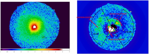
Figure 15. Left panel: 0.5–2 keV XMM MOS image of the galaxy group NGC 5044. Point sources have been removed using the CIAO task dmfilth. An excess of emission in the east direction is clearly seen. Right panel: map of the residuals between the 0.5 and 2 keV MOS image of the left panel and the best fit beta model for the data smoothed on a 20'' scale. The center of NGC 5044 is shown by the red cross and the position and extent of the cold fronts discussed in Gastaldello et al. (2009) are shown by the red arcs. Another relevant feature, the eastern excess, and the sectors used for extraction of the surface brightness profiles discussed in the text are also shown.
Download figure:
Standard image High-resolution imageX-ray sloshing features are witnessing the interaction of the perturber with the group halo. If the perturber as in the case of the three groups discussed above is an optically disturbed spiral galaxy, further constraints might in principle be obtained by comparisons of the optical distortion of the spiral arms produced in simulations following the evolution of disk galaxies within the global tidal field of the group (Villalobos et al. 2012).
10.2. The Low Frequency Radio Emission in IC 1860
Mini radio halos, faint diffuse radio emission with a radius of 100–300 kpc, and a steep spectrum (α ∼ 1.3), are present in a number of relaxed cool-core clusters. The central active galaxies of these clusters are not directly powering the diffuse radio emission as the radiative timescale of the electrons responsible of the observed emission is much shorter than the time required for these electrons to diffuse across the cooling region (Brunetti 2003). Reacceleration of pre-existing, low-energy electrons in the ICM by turbulence in the core region is a possible mechanism responsible for the radio emission. Sloshing motions can produce significant turbulence in the cluster core (Fujita et al. 2004; ZuHone et al. 2013) and this solution is strengthened by the spatial correlation between radio mini-halo emission and cold fronts in some clusters hosting mini-radio halos (Mazzotta & Giacintucci 2008).
An ongoing statistical study of the properties of clusters with and without a minihalo shows that minihalos tend to occur only in very massive, cool-core clusters (S. Giacintucci et al., in preparation). Indeed, no clear detection of a minihalo on the group scale has been reported so far. In IC 1860 we have an indication of a spatial coincidence between a cold front and extended radio emission, similar to what is seen in some minihalo clusters. The GMRT radio emission at 325 MHz is much more extended than the 1.4 GHz emission presented in Dunn et al. (2010) which shows a clear point source with faint extensions in the northeast and southwest directions with no clear correlation with the X-ray extension toward the southeast. Instead, one component of the 325 MHz emission traces the bright tip of the excess spiral feature and is confined within the inner cold front, very much like the spatial coincidence found in clusters with mini radio-halos. Another component is more detached lying in projection at the edge of the spiral. This latter feature resembles the detached components found at 235 MHz in NGC 5044 (Giacintucci et al. 2011; David et al. 2009). However, the extension (only 45 kpc) and the ultra-steep spectral index (α > 1.9) of the radio emission can be explained without the need for in situ re-acceleration as for radio halos and radio mini-halos in galaxy clusters. Indeed, as discussed in Jaffe (1977), a possibility for the transport of the electrons responsible for the radio emission is large-scale motions of the gas carrying the electrons along. ZuHone et al. (2013) showed how relativistic electrons preferentially located in AGN-blown bubbles are redistributed by sloshing motions so that most of them end up within the spiral shape traced out by the cold fronts. Observations at different radio frequencies and simulations tailored for the group's mass scale are needed to investigate the possibility that re-acceleration might take place.
10.3. Reconstructing the Mass Distribution in a Sloshing Group
Since the introduction of the sloshing paradigm in the cluster A1795, it was pointed out that the presence of cold front discontinuities in the ICM density and temperature profiles can cause flawed results in cluster mass estimates (Markevitch et al. 2001). Unphysical discontinuities arise at the cold front in the derived cluster mass profile assuming hydrostatic equilibrium. This is true for most of the published cold front profiles and this fact seems consistent with tangential flows associated with sloshing contributing an additional centrifugal acceleration (Keshet et al. 2010). Roediger et al. (2012b) address the issue of what extent of the underlying mass distribution can be inferred from fully azimuthally averaged temperature and density profiles with the presence of cold fronts in their simulations for the case of the A496 cluster. They found that sloshing modifies the azimuthally averaged profiles by less than 10% and concluded that given the quality of the current available data, the distortion of the profiles due to sloshing does not seem to introduce an observable difference and will not be a major error source for the cluster mass profile. This is also true on the group mass scale. In Gastaldello et al. (2007) this issue was addressed directly in IC 1860 by comparing the mass profile reconstructed in two sectors with P.A. 15°–95° and 195°–15° finding results on the derived total mass (and Navarro–Frenk–White concentration parameter) within their 2σ errors. Therefore the low-level disturbances due to sloshing do not indicate a significant violation of hydrostatic equilibrium.
11. SUMMARY AND CONCLUSIONS
We have presented results of a combined analysis of the currently available XMM and Chandra X-ray data, optical spectroscopy, and radio GMRT for the bright nearby galaxy group IC1860. The results can be summarized as follows.
- 1.The X-ray imaging and spectroscopy reveal the presence of a set of two cold fronts at 45 and 76 kpc and of a spiral of excess surface brightness. Those features are consistent with the sloshing scenario put forward to explain these features, as further supported by the presence of a peculiar velocity of the central galaxy IC 1860 and the identification of a possible perturber in the optically disturbed spiral galaxy IC 1859.
- 2.The analogy of the IC 1860 group with two other X-ray groups showing cold fronts, NGC 5044 and NGC 5846, is tantalizing in terms of the identification of the possible perturber with an optically disturbed spiral galaxy and peculiar velocity of the BCG. We reported further evidence for the sloshing scenario in those two systems. We detected a large scale surface brightness excess in NGC 5044 which strengthen earlier suggestions by David et al. (2009) of the identification of the perturber with the disturbed spiral NGC 5054. We detected hint of a peculiar velocity of the central galaxy NGC 5846.
- 3.The presence of X-ray sloshing features, peculiar velocity of the BCG, and optically disturbed features in the perturbing spiral galaxies are signatures of the interaction of the group tidal field with a disk galaxy and also an indication that this process is actively participating in the transformation of late-type galaxies in the group environment.
- 4.The low frequency GMRT radio data show extended emission with a component confined by the inner cold front as seen in some clusters with mini-halos. Unlike minihalos that require in situ particle reacceleration, the extended emission in IC 1860 is consistent with aged radio plasma redistributed by the sloshing motions.
The case studies presented in this paper show the rich phenomenology and the constraining power that X-ray, optical, and radio data can provide in assessing the dynamical state and past merging history of galaxy groups and their galaxies. We have provided the strongest evidence to date that cold fronts in groups exist and have similar properties to those in massive clusters. This is critical confirmation of the currently favored model of cold-front formation in relaxed objects.
We thank M. Markevitch and T. Venturi for useful discussions and the anonymous referee for suggestions that improved the work presented here. F.G. acknowledges financial contributions by the Italian Space Agency through ASI/INAF agreements I/023/05/0 and I/088/06/0 for the data analysis and I/032/10/0 for the XMM-Newton operations. S.G. acknowledges the support of NASA through Einstein Postdoctoral Fellowship PF0-110071 awarded by the Chandra X-Ray Center (CXC), which is operated by the Smithsonian Astrophysical Observatory (SAO). We are grateful to the ACE SWEPAM instrument team and the ACE Science Center for providing the ACE data and to the 2dF team for the data of the 2dF survey. This research has made use of the NASA/IPAC Extragalactic Database (NED) which is operated by the Jet Propulsion Laboratory, California Institute of Technology, under contract with the National Aeronautics and Space Administration.
APPENDIX A: THE NGC 5044 AND NGC 5846 GROUPS
In this section we report additional X-ray and optical analysis for the NGC 5044 and NGC 5846 groups, which show sloshing cold fronts. The analogy of the IC 1860 group with these systems will reinforce the suggestion of an optically disturbed spiral galaxy as the candidate perturber and provide further evidence of the sloshing scenario on the group scale.
A.1. NGC 5044
The dynamical status of the NGC 5044 group (z = 0.009) as revealed by the presence of cold fronts and sloshing features in its X-ray-emitting gas has been discussed extensively using XMM and Chandra data (Gastaldello et al. 2009; David et al. 2009, and references therein). Here we report additional features in the X-ray morphology in this group, one of the brightest in X-rays, which further support the interpretation of the sloshing scenario and the identification of the perturber.
In the left panel of Figure 15 we report the MOS image of the group already reported in Gastaldello et al. (2009) with a better color coding which highlights the overall extension toward the east direction of the X-ray emission in the 6'–10' (66–110 kpc at the redshift of NGC 5044 for the cosmology adopted in this paper) radial range. In the right panel of Figure 15 we present the surface brightness residual map between the XMM data and the best fit 1D β-model describing the surface brightness radial profile. The cold fronts discovered and discussed in Gastaldello et al. (2009) are shown and the eastern excess clearly stands out in this residual map. The surface brightness profile in Figure 16 show a factor of ∼4 enhancement compared to the symmetrical sector in the west. The presence of almost concentric arcs on opposite sides of the group core and the large-scale asymmetry point toward the orbital plane of the perturber almost parallel to the LOS (e.g., Roediger et al. 2012b, and references therein). The SE (small-scale) spiral feature extending from the SE cold front discussed in David et al. (2009) seems to be a brightness enhancement that connects the inner surface brightness excess marked by the cold front to the large-scale SE excess. The same argument can be made for the NW small spiral, also discussed in David et al. (2009), which seems to connect the core with the NW concentric arc marked by the outer cold front at 67 kpc. These small-scale features are qualitatively seen in simulations and can further constrain the geometry of the merging.

Figure 16. Surface brightness profiles in the angular sectors shown in Figure 15, with position angle measured counterclockwise from the north direction. The surface brightness excess in the east can be seen in the 6'–10' radial range.
Download figure:
Standard image High-resolution imageFrom an optical point of view (see Figure 17) NGC 5044 is also an outstanding object in the local universe for its notable population of dwarf galaxies (e.g., Ferguson & Sandage 1990; Mathews et al. 2004; Faltenbacher & Mathews 2005; Cellone & Buzzoni 2005; Mendel et al. 2008, 2009; Buzzoni et al. 2012). Mendel et al. (2008) using new, deep spectroscopic observations in conjunction with archival velocity information provided a sample of 111 spectroscopically confirmed members. We used that sample to gain further information on the dynamical status of the NGC 5044 group. As already reported by Mendel et al. (2008) the biweight location and scale estimators give a mean group velocity of 2577 ± 33 km s−1 and a velocity dispersion of 331 ± 26 km s−1. Using a velocity for the NGC 5044 galaxy of 2733 ± 51 km s−1 we calculate that its peculiar velocity is 156 ± 61 (just adding errors in quadrature) which corresponds to a Z-score of 0.473 ± 0.098; therefore, the velocity offset is significant at the 4.8σ level.

Figure 17. DSS image of the central region of the NGC 5044 group. NGC 5044 and NGC 5054 are indicated.
Download figure:
Standard image High-resolution imageAs for the candidate perturber, Mendel et al. (2008) reported a low-mass substructure detected by means of the Δ test with six members ∼1.4 Mpc from the group center to the NE. However, as suggested by David et al. (2009), this subgroup is too far away in the outskirts of the group to be a likely candidate, also because it has a very small component of the velocity in the LOS (the biweight mean velocity of the subgroup is 2819 km s−1). A more likely candidate suggested by David et al. (2009) is the giant perturbed spiral NGC 5054 (see Figure 18): it is one of the brightest members of the group and it has a stellar mass of 2.5 × 10¹¹ M☉ comprising 11% of the total stellar mass of the group (Buzzoni et al. 2012). It is at a projected distance of 300 kpc from NGC 5054 and it has a velocity of 1658 km s−1 (Mendel et al. 2008) corresponding to a peculiar velocity of −919 ± 61 km s−1 with respect to the group velocity. At a projected distance of 2 6 (29 kpc) from NGC 5054 lies the Sm/Im galaxy N134, one of the bluest dwarf galaxies of the group, partially overlapping with the north arm; their interaction is likely the cause of the intense star formation activity in N134 and whether or not the interaction is also responsible for the peculiar arm morphology of NGC 5054 is a matter of debate (Buzzoni et al. 2012, and references therein). However, we reinforce David et al.'s (2009) suggestion that NGC 5054 is the likely perturber also given the X-ray evidence presented in Figure 15 and suggest that the peculiar morphology of NGC 5054 is mainly caused by interaction with the global tidal field of the NGC 5044 group halo.

Figure 18. DSS image of the galaxy NGC 5054 together with the companion N134.
Download figure:
Standard image High-resolution imageA.2. NGC 5846
NGC 5846 is a nearby group (z = 0.0056) where evidence for gas sloshing with multiple cold fronts has been presented using a deep (120 ks) Chandra exposure in Machacek et al. (2011). Numerous ring-like structures are present; in particular, the SW feature was already pointed out in the XMM observation presented in Finoguenov et al. (2006). In the left panel of Figure 19 we report the MOS image of the group (taken from the XMM observation ObsID 0021540501) and in the right panel we report the surface brightness residual map between the XMM data and the best fit 1D β-model describing the surface brightness radial profile. The outer cold fronts discussed in Machacek et al. (2011) are shown and the residual map is in agreement with the Chandra one reported in Machacek et al. (2011, see their Figure 4) with a less pronounced tail-like feature given the shorter (15 ks) XMM exposure.

Figure 19. Left panel: 0.5–2 keV XMM MOS image of the galaxy group NGC 5846. Point sources have been removed using the CIAO task dmfilth. An excess of emission is clearly seen in the east direction. Right panel: map of the residuals between the 0.5 and 2 keV MOS image of the left panel and the best fit beta model for the data smoothed on a 20'' scale. The center of NGC 5846 is shown by the red cross and the position and extent of the outer cold fronts discussed in Machacek et al. (2011) are shown by the red arcs.
Download figure:
Standard image High-resolution imageMahdavi et al. (2005) performed a photometric and spectroscopic survey of a 10 deg2 surrounding NGC 5846 and together with ROSAT, XMM, and ASCA data they suggested that NGC 5846 together with the other giant elliptical NGC 5813 are the dominant components of two distinct subgroups separated by 600 kpc in projection and embedded in a larger 1.6 Mpc diameter dark matter halo. Both the NGC 5813 and NGC 5846 galaxy groups are in the ROSAT-ESO Flux-Limited X-Ray catalog (Böhringer et al. 2004). Given the presence of the subgroup associated with NGC 5813 we restricted the spectroscopically confirmed sample of 83 galaxies of Mahdavi et al. (2005) to the members within 400 kpc (0.9 deg) of NGC 5846 resulting in a sample of 39 objects. The biweight location and scale estimators give a mean subgroup velocity of 1833 ± 78 km s−1 and a velocity dispersion of 386 ± 41 km s−1. Using a velocity for the NGC 5846 galaxy of 1714 ± 5 km s−1 (Trager et al. 2000) we calculate that its peculiar velocity is −119 ± 78 corresponding to a Z-score of −0.339 ± 0.206 therefore the velocity offset is marginally significant at the 1.6σ level.
As suggested by Machacek et al. (2011) a likely perturber is the big spiral galaxy NGC 5850 (see Figure 20) which is located 10' (71 kpc) in projection to the east of NGC 5846 and it has a velocity of 2556 ± 4 km s−1 (de Vaucouleurs et al. 1991). It therefore has a relative velocity of 842 ± 6 km s−1 with respect to NGC 5846 and of 723 ± 78 km s−1 with respect to the mean group velocity. The optical image reveal numerous morphological peculiarities, particularly in the spiral arms and structural asymmetries in the H i gas in the direction of NGC 5846 are even more pronounced (Higdon et al. 1998). These features already suggested a recent (≲ 200 Myr) tidal interaction between the two galaxies (Higdon et al. 1998); the new element suggested by the X-ray evidence is that the interaction has been between NGC 5850 and the overall mass of the group halo interior to the orbit of NGC 5850.

Figure 20. DSS image of the central region of the NGC 5846 group. NGC 5846 and NGC 5850 are indicated.
Download figure:
Standard image High-resolution imageAPPENDIX B: REDSHIFT UNCERTAINTIES IN THE CATALOG OF MEMBERS OF THE IC 1860 GROUP
Following Owers et al. (2011b) we performed an independent check of the measured velocities and their uncertainties for the galaxies in the IC 1860 group by cross-correlating the catalogs from different sources. We used as reference the more homogeneous 2dF sample which consists of 74 objects and correlated it with the 6dFGS, the Stein (1996), the Dressler & Shectman (1988), the da Costa et al. (1998), and the RC3 (de Vaucouleurs et al. 1991) redshifts catalogs. The results of the comparisons are shown in Table 4.
Table 4. Comparison of 2dF Redshift Measurements with Literature Values
| Literature Source | Nmatch | σ(Δcz) | Literature Redshift | Quadrature Difference | Ratio | |
|---|---|---|---|---|---|---|
| Uncertainty | ||||||
| (km s−1) | (km s−1) | (km s−1) | ||||
| 6dF | 10 | −17 ± 20 | 52 ± 11 | 31 | 42 ± 14 | 0.35 |
| Stein (1996) | 9 | −7 ± 18 | 60 ± 13 | 23 | 55 ± 14 | 0.26 |
| Dressler & Shectman (1988) | 23 | −61 ± 22 | 90 ± 13 | 45 | 78 ± 15 | 0.50 |
| RC3 | 11 | −30 ± 29 | 75 ± 22 | 43 | 61 ± 27 | 0.48 |
| da Costa et al. (1998) | 14 | −46 ± 19 | 56 ± 15 | 37 | 42 ± 18 | 0.41 |

Notes. Columns are as follows. (1) Origin of external redshift catalog for comparison; (2) number of redshifts in common with the 2dF, Nmatch; (3) the mean redshift difference, , as determined by the biweight estimator; (4) dispersion in the Δcz distribution, σ(Δcz), determined with the biweight estimator; (5) the redshift uncertainty for the external redshift measurements; (6) the quadrature difference between σ(Δcz) and the external redshift error which gives an external estimate of the uncertainty on the 2dF measurements; (7) the ratio of the external uncertainty measurement to the median uncertainty measurement of the 2dF sample which is 89 km s−1. The errors for and σ(Δcz) are obtained as one standard deviation of the distribution obtained by 10,000 bootstrap resamplings of the data.


Download table as: ASCIITypeset image
As can be seen there are no significant offsets from a zero mean for all the redshift differences between the various catalogs, also ensuring that the few external redshifts are consistent with the 2dF ones.
APPENDIX C: THE NARROW-ANGLE-TAIL RADIO GALAXY IC 1858
Radio galaxies located in dense environments often show complex and prominently distorted radio structures. A common morphology is represented by tailed radio galaxies, i.e., double sources whose jets and lobes are bent. Sources whose jets and lobes form a small angle are referred to as narrow-angle-tail radio galaxies (NAT, or U-shaped; Feretti & Venturi 2002, and references therein). Many NAT galaxies reside in clusters, however, an increasing number are found in lower mass environments like groups of galaxies (Freeland et al. 2008, and references therein). Here we report on the GMRT data showing a typical NAT morphology for the IC 1858 galaxy (see left panel of Figure 21). The total flux at 325 MHz is 880 ± 70 mJy and it has a largest angular size of ∼11' corresponding at ∼300 kpc at the redshift of the source. It is also detected in the NVSS with a flux of ∼180 mJy in the same region of the 325 MHz emission (see right panel of Figure 21) implying a spectral index of α ∼ 1.1 typical for such extended sources. Its radio power at 1.4 GHz is 2.0 × 10²³ W Hz−1, again typical for NAT sources. It is at a projected distance of 216 kpc from IC 1860 and it has a velocity difference of −697 ± 99 km s−1 with respect to the mean group velocity. Hence there is a substantial component of the velocity of the galaxy along the LOS; the overall bending of the radio jets points to a component in the plane of the sky pointing in the N–NE direction. The galaxy could therefore just be falling in for the first time, given that it has probably already had time to experience the action of the group environment transforming its morphology into S0, having already experienced its first core passage.

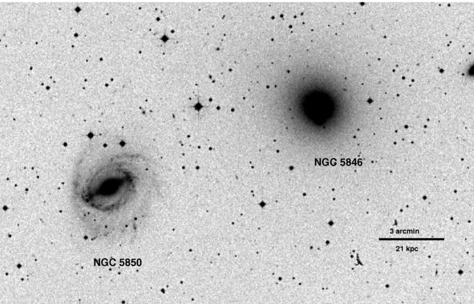
Figure 21. Left panel: GMRT image (contours and gray scale) at 325 MHz of the NAT associated with IC 1858. The restoring beam is 44'' × 40'', in P.A. 0°. The rms noise level is 1 mJy beam−1. Contours are spaced by a factor of two starting from 3 mJy beam−1. The inset shows the GMRT full-resolution (14'' × 9'', −22°) contours overlaid on the DSS image of IC 1858. Contours are spaced by a factor of two starting from 1.2 mJy beam−1. The rms noise level is 0.36 mJy beam−1. Right panel: 1.4 NVSS image of IC 1858. The restoring beam is 45'' × 45'', in P.A. 0°. The rms noise level is 0.5 mJy beam−1. Contours are spaced by a factor of two starting from 1 mJy beam−1.
Download figure:
Standard image High-resolution image
Footnotes
- 15
- 16
- 17
The data are available at http://www.srl.caltech.edu/ACE/.
- 18
The range of the radial bins used for the spectral analysis are: 20''–40''; 40''–60''; 60''–90''; 100''–150''; 180''–230''.
- 19
- 20
We adopt the convention Sν∝ν−α for the synchrotron spectrum, where Sν is the flux density at the frequency ν.