


Abstract
We report multiple lines of evidence for a stochastic signal that is correlated among 67 pulsars from the 15 yr pulsar timing data set collected by the North American Nanohertz Observatory for Gravitational Waves. The correlations follow the Hellings–Downs pattern expected for a stochastic gravitational-wave background. The presence of such a gravitational-wave background with a power-law spectrum is favored over a model with only independent pulsar noises with a Bayes factor in excess of 1014, and this same model is favored over an uncorrelated common power-law spectrum model with Bayes factors of 200–1000, depending on spectral modeling choices. We have built a statistical background distribution for the latter Bayes factors using a method that removes interpulsar correlations from our data set, finding p = 10−3 (≈3σ) for the observed Bayes factors in the null no-correlation scenario. A frequentist test statistic built directly as a weighted sum of interpulsar correlations yields p = 5 × 10⁻⁵ to 1.9 × 10⁻⁴ (≈3.5σ–4σ). Assuming a fiducial f−2/3 characteristic strain spectrum, as appropriate for an ensemble of binary supermassive black hole inspirals, the strain amplitude is  (median + 90% credible interval) at a reference frequency of 1 yr−1. The inferred gravitational-wave background amplitude and spectrum are consistent with astrophysical expectations for a signal from a population of supermassive black hole binaries, although more exotic cosmological and astrophysical sources cannot be excluded. The observation of Hellings–Downs correlations points to the gravitational-wave origin of this signal.
Export citation and abstract BibTeX RIS

Original content from this work may be used under the terms of the Creative Commons Attribution 4.0 licence. Any further distribution of this work must maintain attribution to the author(s) and the title of the work, journal citation and DOI.
1. Introduction
Almost a century had to elapse between Einstein's prediction of gravitational waves (GWs; Einstein 1916) and their measurement from a coalescing binary of stellar-mass black holes (Abbott et al. 2016). However, their existence had been confirmed in the late 1970s through measurements of the orbital decay of the Hulse–Taylor binary pulsar (Hulse & Taylor 1975; Taylor et al. 1979). Today, pulsars are again at the forefront of the quest to detect GWs, this time from binary systems of central galactic black holes.
Black holes with masses of 105–1010 M⊙ exist at the center of most galaxies and are closely correlated with the global properties of the host, suggesting a symbiotic evolution (Magorrian et al. 1998; McConnell & Ma 2013). Galaxy mergers are the main drivers of hierarchical structure formation over cosmic time (Blumenthal et al. 1984) and lead to the formation of close massive black hole binaries long after the mergers (Begelman et al. 1980; Milosavljević & Merritt 2003). The most massive of these (supermassive black hole binaries (SMBHBs), with masses 108–1010 M⊙) emit GWs with slowly evolving frequencies, contributing to a noise-like broadband signal in the nHz range (the GW background (GWB); Rajagopal & Romani 1995; Jaffe & Backer 2003; Wyithe & Loeb 2003; Sesana et al. 2004; McWilliams et al. 2014; Burke-Spolaor et al. 2019). If all contributing SMBHBs evolve purely by loss of circular orbital energy to gravitational radiation, the resultant GWB spectrum is well described by a simple f−2/3 characteristic strain power law (Phinney 2001). However, GWB signals that are not produced by populations of inspiraling black holes may also lie within the nanohertz band; these include primordial GWs from inflation, scalar-induced GWs, and GW signals from multiple processes arising as a result of cosmological phase transitions, such as collisions of bubbles of the post-transition vacuum state, sound waves, turbulence, and the decay of any defects such as cosmic strings or domain walls that may have formed (see, e.g., Guzzetti et al. 2016; Caprini & Figueroa 2018; Domènech 2021, and references therein).
The detection of nanohertz GWs follows the template outlined by Pirani (1956, 2009), whereby we time the propagation of light to measure modulations in the distance between freely falling reference masses. Estabrook & Wahlquist (1975) derived the GW response of electromagnetic signals traveling between Earth and distant spacecraft, sparking interest in low-frequency GW detection. Sazhin (1978) and Detweiler (1979) described nanohertz GW detection using Galactic pulsars and (effectively) the solar system barycenter as references, relying on the regularity of pulsar emission and planetary motions to highlight GW effects. The fact that pulsars are such accurate clocks enables precise measurements of their rotational, astrometric, and binary parameters (and more) from the times of arrival (TOAs) of their pulses, which are used to develop ever-refining end-to-end timing models. Hellings & Downs (1983) made the crucial suggestion that the correlations between the time-of-arrival perturbations of multiple pulsars could reveal a GW signal buried in pulsar noise; Romani (1989) and Foster & Backer (1990) proposed that a pulsar timing array (PTA) of highly stable millisecond pulsars (Backer et al. 1982) could be used to search for a GWB. Nevertheless, the first multipulsar, long-term GWB limits were obtained by analyzing millisecond pulsar residuals independently, rather than as an array (Stinebring et al. 1990; Kaspi et al. 1994).
From a statistical inference standpoint, the problem of detecting nanohertz GWs in PTA data is analogous to GW searches with terrestrial and future space-borne experiments, in which the propagation of light between reference masses is modeled with physical and phenomenological descriptions of signal and noise processes. It is distinguished by the irregular observation times, which encourage a time-domain rather than Fourier-domain formulation, and by noise sources (intrinsic pulsar noise, interstellar-medium-induced radio-frequency-dependent fluctuations, and timing model errors) that are correlated on timescales common to the GWs of interest. This requires the joint estimation of GW signals and noise, which is similar to the kinds of global fitting procedures already used in terrestrial GW experiments and proposed for space-borne experiments. GW analysts have therefore converged on a Bayesian framework that represents all noise sources as Gaussian processes (van Haasteren et al. 2009; van Haasteren & Vallisneri 2014) and relies on model comparison (i.e., Bayes factors, which are ratios of fully marginalized likelihoods) to define detection (see, e.g., Taylor 2021). This Bayesian approach is nevertheless complemented by null hypothesis testing, using a frequentist detection statistic 74 (the "optimal statistic" of Anholm et al. 2009; Demorest et al. 2013; Chamberlin et al. 2015) averaged over Bayesian posteriors of the noise parameters (Vigeland et al. 2018).
The GWB—rather than GW signals from individually resolved binary systems—is likely to become the first nanohertz source accessible to PTA observations (Rosado et al. 2015). Because of its stochastic nature, the GWB cannot be identified as a distinctive phase-coherent signal in the way of individual compact-binary-coalescence GWs. Rather, as PTA data sets grow in extent and sensitivity, one expects to first observe the GWB as excess low-frequency residual power of consistent amplitude and spectral shape across multiple pulsars (Pol et al. 2021; Romano et al. 2021). An observation following this behavior was reported in 2020 (Arzoumanian et al. 2020; hereafter NG12gwb) for the 12.5 yr data set collected by the North American Nanohertz Observatory for Gravitational waves (NANOGrav; McLaughlin 2013; Ransom et al. 2019) and then confirmed (Chen et al. 2021; Goncharov et al. 2021b) by the Parkes PTA (PPTA; Manchester et al. 2013) and the European PTA (EPTA; Desvignes et al. 2016), following many years of null results and steadily decreasing upper limits on the GWB amplitude. A combined International PTA (IPTA; Perera et al. 2019) data release consisting of older data sets from the constituent PTAs also confirmed this observation (Antoniadis et al. 2022). Nevertheless, the finding of excess power cannot be attributed to a GWB origin merely by the consistency of amplitude and spectral shape, which could arise from intrinsic pulsar processes of similar magnitude (Goncharov et al. 2022; Zic et al. 2022), or from a common systematic noise such as clock errors (Tiburzi et al. 2016). Instead, definitive proof of GW origin is sought by establishing the presence of phase-coherent interpulsar correlations with the characteristic spatial pattern derived by Hellings and Downs (Hellings & Downs 1983, hereafter HD): for an isotropic GWB, the correlation between the GW-induced timing delays observed at Earth for any pair of pulsars is a universal, quasi-quadrupolar function of their angular separation in the sky. Even though this correlation pattern is modified if there is anisotropy in the GWB—which may be the case for a GWB generated by an SMBHB population (Cornish & Sesana 2013; Mingarelli et al. 2013, 2017; Taylor & Gair 2013; Mingarelli & Sidery 2014; Roebber & Holder 2017)—the HD template is effective for detecting even anisotropic GWBs in all but the most extreme scenarios (Cornish & Sesana 2013; Cornish & Sampson 2016; Taylor et al. 2020; Bécsy et al. 2022; Allen 2023).
In this letter we present multiple lines of evidence for an excess low-frequency signal with HD correlations in the NANOGrav 15 yr data set (Figure 1). Our key results are as follows. The Bayes factor between an HD-correlated, power-law GWB model and a spatially uncorrelated common-spectrum power-law model ranges from 200 to 1000, depending on modeling choices (Figure 2). The noise-marginalized optimal statistic, which is constructed to be selectively sensitive to HD-correlated power, achieves a signal-to-noise ratio (S/N) of ∼5 (Figures 3 and 4). We calibrated these detection statistics by removing correlations from the 15 yr data set using the phase-shift technique, which removes interpulsar correlations by adding random phase shifts to the Fourier components of the common process (Taylor et al. 2017). We find false-alarm probabilities of p = 10−3 and p = 5 × 10⁻⁵ for the observed Bayes factor and optimal statistic, respectively (see Figure 3).

Figure 1. Summary of the main Bayesian and optimal-statistic analyses presented in this paper, which establish multiple lines of evidence for the presence of Hellings–Downs correlations in the 15 yr NANOGrav data set. Throughout we refer to the 68.3%, 95.4%, and 99.7% regions of distributions as 1σ/2σ/3σ regions, even in two dimensions. (a) Bayesian "free-spectrum" analysis, showing posteriors (gray violins) of independent variance parameters for a Hellings–Downs-correlated stochastic process at frequencies i/T, with T the total data set time span. The blue represents the posterior median and 1σ/2σ posterior bands for a power-law model; the dashed black line corresponds to a γ = 13/3 (SMBHB-like) power law, plotted with the median posterior amplitude. See Section 3 for more details. (b) Posterior probability distribution of GWB amplitude and spectral exponent in an HD power-law model, showing 1σ/2σ/3σ credible regions. The value γGWB = 13/3 (dashed black line) is included in the 99% credible region. The amplitude is referenced to fref = 1 yr−1 (blue) and 0.1 yr−1 (orange). The dashed blue and orange curves in the  subpanel show its marginal posterior density for a γ = 13/3 model, with fref = 1 yr−1 and fref = 0.1 yr−1, respectively. See Section 3 for more details. (c) Angular-separation-binned interpulsar correlations, measured from 2211 distinct pairings in our 67-pulsar array using the frequentist optimal statistic, assuming maximum-a-posteriori pulsar noise parameters and γ = 13/3 common-process amplitude from a Bayesian inference analysis. The bin widths are chosen so that each includes approximately the same number of pulsar pairs, and central bin locations avoid zeros of the Hellings–Downs curve. This binned reconstruction accounts for correlations between pulsar pairs (Romano et al. 2021; Allen & Romano 2022). The dashed black line shows the Hellings–Downs correlation pattern, and the binned points are normalized by the amplitude of the γ = 13/3 common process to be on the same scale. Note that we do not employ binning of interpulsar correlations in our detection statistics; this panel serves as a visual consistency check only. See Section 4 for more frequentist results. (d) Bayesian reconstruction of normalized interpulsar correlations, modeled as a cubic spline within a variable-exponent power-law model. The violins plot the marginal posterior densities (plus median and 68% credible values) of the correlations at the knots. The knot positions are fixed and are chosen on the basis of features of the Hellings–Downs curve (also shown as a dashed black line for reference): they include the maximum and minimum angular separations, the two zero-crossings of the Hellings–Downs curve, and the position of minimum correlation. See Section 3 for more details.
Download figure:
Standard image High-resolution image
Figure 2. Bayes factors between models of correlated red noise in the NANOGrav 15 yr data set (see Section 5.3 and Appendix B). All models feature variable-γ power laws. curn γ is vastly favored over irn (i.e., we find very strong evidence for common-spectrum excess noise over pulsar intrinsic red noise alone); hd γ is favored over curn γ (i.e., we find evidence for Hellings–Downs correlations in the common-spectrum process); dipole and monopole processes are strongly disfavored with respect to curn γ ; adding correlated processes to hd γ is disfavored. While the interpretation of "raw" Bayes factors is somewhat subjective, they can be given a statistical significance within the hypothesis-testing framework by computing their background distributions and deriving the p-values of the observed factors, e.g., Figure 3.
Download figure:
Standard image High-resolution image
Figure 3. Empirical background distribution of hd γ -to-curn γ Bayes factor (left; see Section 3) and noise-marginalized optimal statistic (right; see Section 4), as computed by the phase-shift technique (Taylor et al. 2017) to remove interpulsar correlations. We only compute 5000 Bayesian phase shifts, compared to 400,000 optimal statistic phase shifts, because of the huge computational resources needed to perform the Bayesian analyses. For the optimal statistic, we also compute the background distribution using 27,000 simulations (orange line) and compare to an analytic calculation (green line). Dotted lines indicate Gaussian-equivalent 2σ, 3σ, and 4σ thresholds. The dashed vertical lines indicate the values of the detection statistics for the unshifted data sets. For the Bayesian analyses, we find p = 10−3 (≈3σ); for the optimal statistic analyses, we find p = 5 × 10⁻⁵ to 1.9 × 10⁻⁴ (≈3.5σ–4σ).
Download figure:
Standard image High-resolution imageFor our fiducial power-law model (f−2/3 for characteristic strain and f−13/3 for timing residuals) and a log-uniform amplitude prior, the Bayesian posterior of GWB amplitude at the customary reference frequency 1 yr−1 is  (median with 90% credible interval), which is compatible with current astrophysical estimates for the GWB from SMBHBs (e.g., Burke-Spolaor et al. 2019; Agazie et al. 2023b). This corresponds to a total integrated energy density of
  or
or  (assuming H0 = 70 km s−1 Mpc−1) in our sensitive frequency band. For a more general model of the timing-residual power spectral density with variable power-law exponent −γ, we find
  and
and  . See Figure 1(b) for AGWB and γ posteriors. The posterior for γ is consistent with the value of 13/3 predicted for a population of SMBHBs evolving by GW emission, although smaller values of γ are preferred; however, the recovered posteriors are consistent with predictions from astrophysical models (see Agazie et al. 2023b). We also note that, unlike our detection statistics (which are calibrated under our modeling assumptions), the estimation of γ is very sensitive to minor details in the data model of a few pulsars.
The rest of this paper is organized as follows. We briefly describe our data set and data model in Section 2. Our main results are discussed in detail in Sections 3 and 4; they are supported by a variety of robustness and validation studies, including a spectral analysis of the excess signal (Section 5.2), a correlation analysis that finds no significant evidence for additional spatially correlated processes (Section 5.3), and cross-validation studies with single-telescope data sets and leave-one-pulsar-out techniques (Section 5.4). In the past 2 yr we have performed an end-to-end review of the NANOGrav experiment, to identify and mitigate possible sources of systematic error or data set contamination; our improvements and considerations are partly described in a set of companion papers: on the NANOGrav statistical analysis as implemented in software (A. Johnson et al. 2023, in preparation), on the 15 yr data set (Agazie et al. 2023a, hereafter NG15), and on pulsar models (Agazie et al. 2023c, hereafter NG15detchar). More companion papers address the possible SMBHB (Agazie et al. 2023b) and cosmological (Afzal et al. 2023) interpretations of our results, with several more GW searches and signal studies in preparation. We look forward to the cross-validation analysis that will become possible with the independent data sets collected by other IPTA members.
2. The 15 yr Data Set and Data Model
The NANOGrav 15 yr data set 75 (NG15) contains observations of 68 pulsars obtained between 2004 July and 2020 August with the Arecibo Observatory (Arecibo), the Green Bank Telescope (GBT), and the Very Large Array (VLA), augmenting the 12.5 yr data set (Alam et al. 2021a, 2021b) with 2.9 yr of timing data for the 47 pulsars in the previous data set, and with 21 new pulsars. 76 For this paper we analyze narrowband TOAs, which are computed separately for subbands of each receiver, and focus on the 67 pulsars with a timing baseline ≥3 yr. We adopt the TT(BIPM2019) timescale and the JPL DE440 ephemeris (Park et al. 2021), which improves Jupiter's orbit with ranging and very long baseline interferometry observations of the Juno spacecraft. Uncertainties in the Jovian orbit impacted NANOGrav's 11 yr GWB search (Arzoumanian et al. 2018; Vallisneri et al. 2020), but they are now negligible.
For each pulsar, we fit the TOAs to a timing model that includes pulsar spin period, spin period derivative, sky location, proper motion, and parallax. While not all pulsars have measurable parallax and proper motion, we always include these parameters because they induce delays with the same frequencies for all pulsars (f = 0.5 yr−1 for parallax and f = yr−1 plus a linear envelope for proper motion), so there is a risk that a parallax or proper-motion signal could be misidentified as a GW signal. Fitting for these parameters in all pulsars reduces our sensitivity to GWs at those frequencies; however, this effect is minimal for GWB searches since these frequencies are much higher than the frequencies at which we expect the GWB to be significant. For binary pulsars, the timing model includes also five orbital elements for binary pulsars and additional non-Keplerian parameters when these improve the fit as determined by an F-test. We fit variations in dispersion measure (DM) as a piecewise-constant "DMX" function (Arzoumanian et al. 2015; Jones et al. 2017). The individual analysis of each pulsar provides best-fit estimates of the timing residuals δ t , of white measurement noise, and of intrinsic red noise, modeled as a power law (Cordes 2013; Jones et al. 2017; Lam et al. 2017). 77 White measurement noise is described by three parameters: a linear scaling of TOA uncertainties ("EFAC"), white noise added to the TOA uncertainties in quadrature ("EQUAD"), and noise common to all subbands at the same epoch ("ECORR"), with independent parameters for every receiver/back-end combination (see NG15detchar). We summarize white noise by its maximum a posteriori (MAP) covariance C . See Appendix A for more details of our instruments, observations, and data reduction pipeline; a complete discussion of the data set can be found in NG15.
In our Bayesian GWB analysis, we model
δ
t
as a finite Gaussian process consisting of time-correlated fluctuations that include intrinsic red pulsar noise and (potentially) a GW signal, along with timing model uncertainties (van Haasteren et al. 2009; van Haasteren & Vallisneri 2014; Taylor 2021). The red noise is modeled with Fourier basis
F
and amplitudes
c
(Lentati et al. 2013). All Fourier bases (the columns of
F
) are sines and cosines computed on the TOAs with frequencies fi
= i/T, where T = 16.03 yr is the TOA extent. The timing model uncertainties are modeled with design matrix basis
M
and coefficients
 . The single-pulsar log likelihood is then

with

The prior for the
is taken to be uniform with infinite extent, so the posterior is driven entirely by the likelihood. The set of the {
c
} for all pulsars take a joint normal prior with zero mean and covariance

here a, b range over pulsars and i, j over Fourier components, and δij
is Kronecker's delta. The term φai
describes the spectrum of intrinsic red noise in pulsar a, while Φab,i
describes processes with common spectrum across all pulsars and (potentially) phase-coherent interpulsar correlations. The {
c
} prior ties together the single-pulsar likelihoods given by Equation (1) into a joint posterior, p(
c
,
,
η
∣
δ
t
) ∝ p(
δ
t
∣
c
,
)p(
c
,
∣
η
)p(
η
), where we have dropped subscripts to denote the concatenation of vectors for all pulsars, and where
η
denotes all the hyperparameters (such as red-noise and GWB power-spectrum amplitudes) that determine the covariances. We marginalize over
c
and
analytically and use Markov chain Monte Carlo (MCMC) techniques (see Appendix B) to estimate p(
η
∣
δ
t
) for different models of the intrinsic red noise and common spectrum.
The data model variants adopted in this paper all share this probabilistic setup but differ in the structure and parameterization of Φab,i . For a model with intrinsic red noise only (henceforth irn), Φab,i = 0; for common-spectrum spatially uncorrelated red noise (curn), Φab,i = δab ΦCURN,i ; for an isotropic GWB with Hellings–Downs correlations (hd), Φab,i = Γ(ξab )ΦHD,i , with Γ the Hellings–Downs function of pulsar angular separations ξab ,


In NG12gwb we established strong Bayesian evidence for curn over irn; finding that hd is preferred over curn would point to the GWB origin of the common-spectrum signal. We also investigate other spatial correlation patterns, e.g., monopole or dipole, introduced in Section 5.3.
Throughout this paper, we set the spectral components φai of intrinsic pulsar noise (which have units of s2, as appropriate for the variance of timing residuals) to a power law,
introducing two dimensionless hyperparameters for each pulsar: the intrinsic noise amplitude Aa and spectral index γa . We use log-uniform and uniform priors, respectively, on these hyperparameters; their bounds are described in Appendix B. More sophisticated intrinsic noise models are discussed in Section 5.1 and NG15detchar. In models curn γ and hd γ , the common spectra ΦCURN,i and ΦHD,i follow Equation (6),
introducing hyperparameters ACURN, γCURN and AHD, γHD, respectively. However, we set γHD = 13/3 for the GWB from a stationary ensemble of inspiraling binaries and refer to that fiducial model as hd 13/3. For specific "free-spectrum" studies we will instead model the individual ΦCURN,i or ΦHD,i elements and refer to models curn free and hd free. Throughout this article we use frequencies fi = i/T with i = 1–30 for intrinsic noise (f = 2–59 nHz), covering a frequency range over which pulsar noise transitions from red noise dominated to white noise dominated. For common-spectrum noise, we limit the frequency range in order to reduce correlations with excess white noise at higher frequencies. Following NG12gwb, we fit a curn γ model enhanced with a power-law break to our data and limit frequencies to the MAP break frequencies (i = 1–14 or f = 2–28 nHz; see Appendix C).
3. Bayesian Analysis
When fit to the 15 yr data set, the curn
γ
and hd
γ
models agree on the presence of a loud time-correlated stochastic signal with common amplitude and spectrum across pulsars.
78
The joint AHD– γHD Bayesian posterior is shown in Figure 1(b), with 1D marginal posteriors in the horizontal and vertical subplots. The posterior medians and 5%–95% quantiles are  and
and  . The thicker curve in the vertical subplot is the AHD posterior for the hd
13/3 model, for which
. The thicker curve in the vertical subplot is the AHD posterior for the hd
13/3 model, for which  . These amplitudes are compatible with astrophysical expectations of a GWB from inspiraling SMBHBs (see Section 6). The AHD posterior has essentially no support below 10−15.
The strong AHD– γHD correlation is an artifact of using the fref = 1 yr−1 in Equation (6), and it largely disappears when fref is moved to the band of greatest PTA sensitivity; see the dashed contours in Figure 1(b) for fref = (10 yr)−1. The γHD posterior is in moderate tension with the theoretical universal binary inspiral value γHD = 13/3, which lies at the 99% credible boundary: smaller values of γHD could be an indication that astrophysical effects, such as stellar scattering and gas dynamics, play a role in the evolution of SMBHBs emitting GWs in this frequency range (see Section 6; Agazie et al. 2023b). This highlights the importance of measuring this parameter. Furthermore, its estimation is sensitive to details in the modeling of intrinsic red noise and of interstellar medium timing delays in a few pulsars (see the analysis in Section 5.2). Notably, in the 12.5 yr data set γHD = 13/3 was recovered at ∼1σ below the median (NG12gwb); this anomaly is reversed in the newer data set. It is likely that more expansive data sets or more sophisticated chromatic noise models, e.g., next-generation Gaussian process models such as in Section 5.1 (Lam et al. 2018; Goncharov et al. 2021a; Chalumeau et al. 2022), will be needed to infer the presence of possible systematic errors in γHD.
Our Bayesian analysis provides evidence that the common-spectrum signal includes Hellings–Downs interpulsar correlations. Specifically, the Bayes factor between the hd γ and curn γ models ranges from 200 (when 14 Fourier frequencies are included in Φi ) to 1000 (when five frequencies are included, as in NG12gwb). Results are similar for hd 13/3 versus curn 13/3. Figure 2 recapitulates Bayes factors between a variety of models, including some with the alternative spatial correlation structures discussed in Section 5.3. The very peaked AHD posterior in Figure 1(b), significantly separated from smaller amplitudes, supports the very large Bayes factor between irn and curn γ . The 15 yr data set favors hd γ over curn γ , as well as over models with monopolar or dipolar correlations, and it is inconclusive about, i.e., gives roughly even odds for, the presence of spatially correlated signals in addition to hd γ .
We can also regard the hd γ versus curn γ Bayes factor as a detection statistic in a hypothesis-testing framework and derive the p-value of the observed Bayes factor with respect to its empirical distribution under the curn γ model. We do so by computing Bayes factors on 5000 bootstrapped data sets where interpulsar spatial correlations are removed by introducing random phase shifts, drawn from a uniform distribution from 0 to 2π, to the common-process Fourier components (Taylor et al. 2017). This procedure alters interpulsar correlations to have a mean of zero, while leaving the amplitudes of intrinsic pulsar noise and CURN unchanged, thus providing a way to test the null hypothesis that no interpulsar correlations are present. The resulting background distribution of Bayes factors is shown in the left panel of Figure 3—they exceed the observed value in 5 of the 5000 phase shifts (p = 10−3). We also performed sky scramble analyses (Cornish & Sampson 2016), which remove the dependence of interpulsar spatial correlations on the angular separations between the pulsars by attributing random sky positions to the pulsars. Sky scrambles generate a background distribution for which interpulsar correlations are present in the data, but they are independent of the pulsars' angular separations; for this distribution, we find p = 1.6 × 10⁻³. A detailed discussion of sky scrambles and the results of these analyses can be found in Appendix F.
As in NG12gwb, we also carried out a minimally modeled Bayesian reconstruction of the interpulsar correlation pattern, using spline interpolation over seven spline-knot positions. The choice of seven spline-knot positions is based on features of the Hellings–Downs pattern: two correspond to the maximum and minimum angular separations (0° and 180°, respectively), two are chosen to be at the theoretical zero-crossings of the Hellings–Downs pattern (49.2° and 121.8°), one is at the theoretical minimum (82.5°), and the final two are between the end points and zero-crossings (25° and 150°) to allow additional flexibility in the fit. Figure 1(d) shows the marginal 1D posterior densities at these spline-knot positions for a power-law varied-exponent model. The reconstruction is consistent with the overplotted Hellings–Downs pattern; furthermore, the joint 2D marginal posterior densities for the knots, not shown in Figure 1(d), at the HD zero-crossings are consistent with (0, 0) within 1σ credibility.
4. Optimal Statistic Analysis
We complement our Bayesian search with a frequentist analysis using the optimal statistic (Anholm et al. 2009; Demorest et al. 2013; Chamberlin et al. 2015), a summary statistic designed to measure correlated excess power in PTA residuals. (Note that there is no accepted definition of "optimal statistic" in modern statistical usage, but the term has become established in the PTA literature to refer to this specific method, so we use it for this reason.) It is enlightening to describe the optimal statistic as a weighted average of the interpulsar correlation coefficients
where  are the residuals of pulsar a and
  is their total autocovariance matrix. The cross-covariance matrix
  encodes the spectrum of the HD-correlated signal, normalized so that
  (see Pol et al. 2022), and where elements of Φab
are given by Equation (3). Indeed, the ρab
have expectation value A2Γ(ξab
), but their variance
(see Pol et al. 2022), and where elements of Φab
are given by Equation (3). Indeed, the ρab
have expectation value A2Γ(ξab
), but their variance  is too large to use them directly as estimators. Thus, we assemble the optimal statistic as the variance-weighted, Γ-template-matched average of the ρab
,
is too large to use them directly as estimators. Thus, we assemble the optimal statistic as the variance-weighted, Γ-template-matched average of the ρab
,
This equation represents the optimal estimator of the HD amplitude A2; it can also be interpreted as the best-fit  obtained by least-squares fitting the ρab
to the Hellings–Downs model
obtained by least-squares fitting the ρab
to the Hellings–Downs model  . Because
  is a function of intrinsic red noise and common-process hyperparameters through the
  , we use the results of an initial Bayesian inference run to refer the statistic to MAP hyperparameters, or to marginalize it over their posteriors. As discussed in Vigeland et al. (2018), we obtain more accurate values of the amplitude by this marginalization.
To search for interpulsar correlations using the optimal statistic, we evaluate the frequency (the p-value) with which an uncorrelated common-spectrum process with parameters estimated from our data set would yield  greater than we observe. In the absence of a signal, the expectation value of
  is zero, and its distribution is approximately normal. Thus, we divide the observed
  by its standard deviation to define a formal S/N
Figure 4 shows the distribution of this S/N over curn γ and curn 13/3 noise parameter posteriors, with S/Ns of 5 ± 1 and 4 ± 1, respectively (means ± standard deviations across noise parameter posteriors). We use 14 frequency components to model the signal; the dependence on the number of frequency components is very weak.

Figure 4. Optimal statistic S/N for HD correlations, distributed over curn γ (solid lines) and curn 13/3 (dashed lines) noise parameter posteriors. The vertical lines indicate the mean S/Ns. We find S/Ns of 5 ± 1 and 4 ± 1 for curn γ and curn 13/3, respectively.
Download figure:
Standard image High-resolution imageBecause the distribution of  is only approximately normal (Hazboun et al. 2023), the S/N of Equation (11) does not map analytically to a p-value, and it cannot be interpreted as a "sigma" level. Instead, optimal statistic p-values can be computed empirically by removing interpulsar correlations from the 15 yr data set with phase shifts (Taylor et al. 2017). We draw random phase offsets from 0 to 2π for the common-process Fourier components, which is equivalent to making uniform draws from the background distribution of CURN, and ask how often a random choice of phase offsets produces an HD-correlated signal. The right panel of Figure 3 shows the distribution of noise-marginalized S/N over 400,000 phase shifts. There are 19 phase shifts with noise-marginalized S/N greater than observed, with p = 5 × 10⁻⁵. We compare the phase-shift distribution with backgrounds obtained by simulation (right panel of Figure 3, orange line) and analytic calculation (green line). For the former, we simulate 27,000 curn
γ
realizations using MAP hyperparameters from the 15 yr data and compute the optimal statistic S/N for each; for the latter, we evaluate the generalized χ2 distribution (Hazboun et al. 2023) with median curn
γ
hyperparameters. Although neither method includes the marginalization over noise parameter posteriors, we find good agreement with phase shifts, with p = 1.8 × 10⁻⁴ from simulations and p = 1.9 × 10⁻⁴ from the analytic calculation. Finally, we use sky scrambles to compute the p-value for the null hypothesis that interpulsar correlations are present, but they have no dependence on the angular separation between the pulsars, for which we find p < 10−4 (see Appendix F).
is only approximately normal (Hazboun et al. 2023), the S/N of Equation (11) does not map analytically to a p-value, and it cannot be interpreted as a "sigma" level. Instead, optimal statistic p-values can be computed empirically by removing interpulsar correlations from the 15 yr data set with phase shifts (Taylor et al. 2017). We draw random phase offsets from 0 to 2π for the common-process Fourier components, which is equivalent to making uniform draws from the background distribution of CURN, and ask how often a random choice of phase offsets produces an HD-correlated signal. The right panel of Figure 3 shows the distribution of noise-marginalized S/N over 400,000 phase shifts. There are 19 phase shifts with noise-marginalized S/N greater than observed, with p = 5 × 10⁻⁵. We compare the phase-shift distribution with backgrounds obtained by simulation (right panel of Figure 3, orange line) and analytic calculation (green line). For the former, we simulate 27,000 curn
γ
realizations using MAP hyperparameters from the 15 yr data and compute the optimal statistic S/N for each; for the latter, we evaluate the generalized χ2 distribution (Hazboun et al. 2023) with median curn
γ
hyperparameters. Although neither method includes the marginalization over noise parameter posteriors, we find good agreement with phase shifts, with p = 1.8 × 10⁻⁴ from simulations and p = 1.9 × 10⁻⁴ from the analytic calculation. Finally, we use sky scrambles to compute the p-value for the null hypothesis that interpulsar correlations are present, but they have no dependence on the angular separation between the pulsars, for which we find p < 10−4 (see Appendix F).
Averaging the cross-correlations ρab in angular separation bins with equal numbers of pulsar pairs reveals the Hellings–Downs pattern, as shown in Figure 1(c) for 15 bins. The ρab were evaluated with MAP curn 13/3 noise parameters. The black dashed curve traces the expected correlations for an HD-correlated background with the MAP amplitude; the vertical error bars display the expected 1σ spreads of the binned cross-correlations, accounting for the 〈ρab ρcd 〉 covariances induced by the HD-correlated process (Romano et al. 2021; Allen & Romano 2022). (Neglecting those covariances yields 20%–40% smaller spreads. Note that they are not included in p-value estimates because those are calculated under the null hypothesis of no spatially correlated process.)
Although each draw from the noise parameter posterior would generate a slightly different plot, as would different binnings, the quality of the fit seen in Figure 1 provides a visual indication that the excess low-frequency power in the 15 yr data set harbors HD correlations. The χ2 for this 15-bin reconstruction with respect to the Hellings–Downs curve is 8.1, where we account for ρab covariance in constructing the bins and the covariance between bins in constructing the χ2 (Allen & Romano 2022). This corresponds to a p-value of 0.75, calculated using simulations based on the hd γ model, or 0.92 if one assumes that this value follows a canonical χ2 with 15 degrees of freedom. These p-values are representative of what we find with different binnings: we find p > 0.3 when using 8–20 bins (assuming a canonical χ2 distribution).
5. Checks and Validation
Prior to analyzing the 15 yr data set, we extensively reviewed our data collection and analysis procedures, methods, and tools, in an effort to eliminate contamination from systematic effects and human error. Furthermore, the results presented in Sections 3 and 4 are supported by a variety of consistency checks and auxiliary studies. In this section we present those that offer evidence for or against the presence of HD correlations, reveal anomalies, or otherwise highlight features of note in the data: alternative DM modeling (Section 5.1), the spectral content (Section 5.2), and correlation pattern (Section 5.3) of the excess-noise signal, as well as the consistency of our findings across data set "slices," pulsars, and telescopes (Section 5.4).
5.1. Alternative DM Models
In this paper and in previous GW searches (e.g., NG12gwb), we model fluctuations in the DM using DMX parameters (a piecewise-constant representation; see NG15). Adopting this DM model as the standard makes it easier to directly compare the results here to those in NG12gwb. An alternative model where DM variations are modeled as a Fourier-domain Gaussian process, DMGP, has been used by Antoniadis et al. (2022), Chen et al. (2021), and Goncharov et al. (2021b). The Fourier coefficients follow a power law similar to those of intrinsic and common-spectrum red noise, but their basis vectors include a ν−2 radio frequency dependence, and the component frequencies fi = i/T range through i = 1–100. Under the DMGP model we also include a deterministic solar-wind model (Hazboun et al. 2022) and the two chromatic events in PSR J1713+0747 reported in Lam et al. (2018), which are modeled as deterministic exponential dips with the chromatic index quantifying the radio frequency dependence of the dips left as a free parameter. If these chromatic events are not modeled, they raise estimated white noise (Hazboun et al. 2020). A detailed discussion of chromatic noise effects can be found in NG15detchar.
Using the DMGP model in place of DMX has minimal effects on nearly all pulsars in the array. Only PSR J1713+0747 and PSR J1600−3053 show notable differences in their recovered intrinsic noise parameters. However, DMGP does affect the parameter estimation of common red noise, as seen in Figure 5, shifting the posterior for γ to higher values that are more consistent with 13/3. Despite this, we still recover HD correlations at the same significance as when we use DMX to model fluctuations in the DM, implying that the evidence reported for the presence of correlations in this work is independent of the choice of DM noise modeling.

Figure 5. curn γ posterior distributions using DMGP (red) and DMX (blue) to model DM variations. The dashed line marks γCURN = 13/3. While the posteriors are broadly consistent, DMGP shifts the γCURN posterior to higher values, making it more consistent with γCURN = 13/3.
Download figure:
Standard image High-resolution image5.2. Spectral Analysis
Adopting power-law spectra for curn and hd is a useful simplification that reduces the number of fit parameters and yields more informative constraints; furthermore, it is expedient to identify hd 13/3 with the hypothesis that we are observing the GWB from SMBHBs. Nevertheless, the standard γ = 13/3 power law for GW inspirals may be altered by astrophysical processes such as stellar and gas friction in nuclei (see, e.g., Merritt & Milosavljević 2005 for a review), by appreciable eccentricity in SMBHB orbits (Enoki & Nagashima 2007), and by low-number SMBHB statistics (Sesana et al. 2008). hd γ parameter recovery may also be biased if intrinsic pulsar noise is not modeled well by a power law. Indeed, our data show hints of a discrepancy from the idealized hd 13/3 model: the γHD posterior in Figure 1(b) favors slopes much shallower than 13/3, and the hd γ -to-curn γ Bayes factor drops from 1000 to 200 when Fourier components at more than five frequencies are included in the model.
We examine the spectral content of the 15 yr data set using the curn free and hd free models, which are parameterized by the variances of the Fourier components at each frequency. Their marginal posteriors are shown in the left panel of Figure 6, where bin number i corresponds to fi = i/T, with T = 16.03 yr the extent of the data set. For the purpose of illustration, we overlay best-fit power laws that thread the posteriors in a way similar to the factorized PTA likelihood of Taylor et al. (2022) and Lamb et al. (2023).

Figure 6. Left: posteriors of Fourier component variance Φi for the curn free (left) and hd free (right) models (see Section 2), plotted at their corresponding frequencies fi = i/T, with T the 16.03 yr extent of the data set. Excess power is observed in bins 1–8 (somewhat marginally in bin 6); Hellings–Downs-correlated power in bins 1–5 and 8. The dashed line plots the best-fit power law, which has γ ≃ 3.2 (as in Figure 1(d)); the fit is pushed to lower γ by bins 1 and 8. The dotted line plots the best-fit power law when γ is fixed to 13/3; it overshoots in bin 1 and undershoots in bin 8. Right: posteriors of variance Φ2 in Fourier bin 2 (f2 = 3.95 nHz) in a curn free + hd free + monopole free + dipole free model, showing evidence of a quasi-monochromatic monopole process (dashed). No monopole or dipole power is observed in all other bins of that joint model, with ΦCURN,i and ΦHD,i posteriors consistent with the left panel.
Download figure:
Standard image High-resolution imageWe deem excess power, either uncorrelated for curn free or correlated for hd free, to be observed in a bin when the support of the posterior is concentrated away from the lowest amplitudes. No power of either kind is observed above f8, consistent with the presence of a floor of white measurement noise. Furthermore, no correlated power is observed in bins 6 and 7, where a power-law model would expect a smooth continuation of the trend of bins 1–5 (see the dashed fit of Figure 6); this may explain the drop in the Bayes factor. However, correlated power reappears in bin 8, pushing the fit toward shallower slopes. Indeed, repeating the fit by omitting subsets of the bins suggests that the low recovered γHD is due mostly to bin 8 and to the lower-than-expected correlated power found in bin 1. Obviously, excluding those bins leads to higher γHD estimates.
To explore deviations from a pure power law that may arise from statistical fluctuations of the astrophysical background or from unmodeled systematics (perhaps related to the timing model), in Appendix D we relax the normal ck
prior (see Equation (3)) to a multivariate Student's t-distribution that is more accepting of mild outliers. The resulting estimate of γCURN peaks at a higher value and is broader than in curn
γ
, with posterior medians and 5%–95% quantiles of  .
.
Similarly, spectral turnovers due to interactions between SMBHBs and their environments can result in reduced GWB power at lower frequencies, which might explain the slightly lower correlated power in bin 1. We investigate this hypothesis in Appendix E using the turnover spectrum of Sampson et al. (2015). For this curn turnover model, the 15 yr data favor a spectral bend below 10 nHz (near f5), but the Bayes factor against the standard hd γ is inconclusive.
Future data sets with longer time spans and the comparison of our data set with those of other PTAs should help clarify the astrophysical or systematic origin of these possible spectral features.
5.3. Alternative Correlation Patterns
Sources other than GWs can produce interpulsar residual correlations with spatial patterns other than HD. For example, errors in the solar system ephemerides create time-dependent Roemer delays with dipolar correlations (Roebber 2019; Vallisneri et al. 2020), and errors in the correction of telescope time to an inertial timescale (Hobbs et al. 2012, 2020) create an identical time-dependent delay for all pulsars (i.e., a delay with monopolar correlations).
Gair et al. (2014) showed that, for a pulsar array distributed uniformly across the sky, HD correlations can be decomposed as
where the  are Legendre polynomials of order l evaluated at the pulsar angular separation ξab
. In other words, an HD-correlated signal should have no power at l = 0 or l = 1.
are Legendre polynomials of order l evaluated at the pulsar angular separation ξab
. In other words, an HD-correlated signal should have no power at l = 0 or l = 1.
We can perform a frequentist generic correlation search using Legendre polynomials
79
with the multiple-component optimal statistic (MCOS; Sardesai & Vigeland 2023)—a generalized statistic that allows multiple correlation patterns to be fit simultaneously to the correlation coefficients ρab
. Figure 7 shows the constraints on  obtained by fitting the correlations ρab
to this Legendre series using the MCOS and marginalizing over curn
γ
noise parameter posteriors. The quadrupolar structure of the data is evident, along with a small but significant monopolar contribution.
obtained by fitting the correlations ρab
to this Legendre series using the MCOS and marginalizing over curn
γ
noise parameter posteriors. The quadrupolar structure of the data is evident, along with a small but significant monopolar contribution.

Figure 7. Multiple-component optimal statistic for a Legendre polynomial basis Equation (12) with  . The violin plots show the distributions of the normalized Legendre coefficients
  over curn
γ
noise parameter posteriors. The black dashed line shows the Legendre spectrum of a pure-HD signal, with the median posterior
over curn
γ
noise parameter posteriors. The black dashed line shows the Legendre spectrum of a pure-HD signal, with the median posterior  .
.
Download figure:
Standard image High-resolution imageThe same feature from the Legendre decomposition appears if we use the MCOS to search for multiple correlations simultaneously: a multiple regression analysis favors models that contain both significant HD and monopole correlations (see Appendix G). From simulations of 15 yr–like data sets (see Appendix H.1), we find a p-value of 0.11 (~2σ) for observing a monopole at this significance or higher with a pure-HD injection of amplitude similar to what we observe. We also perform a model-checking study to assess whether the observed monopole is consistent with the hd 13/3 model (see Appendix H.2), and we find a p-value of 0.11 for producing an apparent monopole when the signal is purely hd 13/3. Thus, we conclude that it is possible for an HD-correlated signal to appear to have monopole correlations in an optimal statistic analysis at this significance level.
In contrast, Bayesian searches for additional correlations do not find evidence of additional monopole- or dipole-correlated red-noise processes; as shown in Figure 2, the Bayes factors for these processes are ∼1. We also perform a general Bayesian search for correlations using a curn free + hd free + monopole free + dipole free model, which allows for independent uncorrelated and correlated components at every frequency bin. We note that this analysis is more flexible than the ones described above, which assume a power-law power spectral density. We find no significant dipole-correlated power at any frequency, and we find monopole-correlated power only in the second frequency bin (f2 = 3.95 nHz); posteriors of variance for that bin are shown in the right panel of Figure 6.
Motivated by this finding, we perform a search for hd γ + sinusoid, which includes a deterministic sinusoidal delay (applied to all pulsars alike, as appropriate for a monopole) with free frequency, amplitude, and phase. The sinusoid's posteriors match the free-spectral analysis in frequency and amplitude; however, the Bayes factor between hd γ + sinusoid and hd γ calculated using two methods (Hee et al. 2015; Hourihane et al. 2023) is only ∼1, so the signal cannot be considered statistically significant. Astrophysically motivated searches for sources that produce sinusoidal or sinusoid-like delays in the residuals, such as an individual SMBHB or perturbations to the local gravitational field induced by fuzzy dark matter (Khmelnitsky & Rubakov 2014), also yield Bayes factors ∼1. Thus, we conclude that there is some evidence of additional power at 3.95 nHz with monopole correlations; however, the significance in the Bayesian analyses is low, while the optimal statistic S/N could be produced by an HD-correlated signal. Therefore, we cannot definitively say whether the signal is present, or determine the source. We note that performing an MCOS analysis after subtracting off realizations of a sinusoid using hd γ + sinusoid posteriors reduces the (S/N)monopole ≃ 0 while (S/N)HD remains unchanged, indicating that this single-frequency monopole-correlated signal is likely causing the nonzero monopole signal observed in the MCOS analysis.
Similar hints of a monopolar signal (though weaker) were found in the NANOGrav 12.5 yr data set, unsurprisingly given that it is a subset of the current data set. To exercise due diligence, we audited the correction of telescope time to GPS time at Arecibo and at GBT and found nothing that could explain our observations. The subsequent steps in the time correction pipeline rely on very accurate atomic clocks and are unlikely to introduce considerable systematics (G. Petit 2022, personal communication). An important test will be whether this signal persists in future data sets. If this monopolar feature is truly an astrophysical signal, we would expect it to increase in significance as our data set grows. Comparisons with other PTAs and combined IPTA data sets will also provide crucial insight.
5.4. Dropout and Cross-validation
The GWB is by its nature a signal affecting all of the pulsars in the PTA, although it may appear more significant in some based on their observing time span, noise properties, and the particular realization of pulsar and Earth contributions (Speri et al. 2023). One way to assess the significance of the GWB in each pulsar is a Bayesian dropout analysis (Aggarwal et al. 2019; Arzoumanian et al. 2020), which introduces a binary parameter that turns on and off the common signal (or its interpulsar correlations) for a single pulsar, leaving all other pulsars unchanged. The Bayes factor associated with this parameter, also referred to as the "dropout factor," describes how much each pulsar likes to "participate" in the common signal.
Figure 8 plots curn γ versus irn dropout factors for all 67 pulsars (blue). We find positive dropout factors (i.e., dropout factors >2) for an uncorrelated common process in 20 pulsars, while only one has a dropout factor <0.5. For comparison, in the NANOGrav 12.5 yr data set 10 pulsars showed positive dropout factors for an uncorrelated common process, while three had negative dropout factors. We also show HD correlations versus curn γ dropout factors (orange). For these, the uncorrelated common process is always present in all pulsars, but the cross-correlations for all pulsar pairs involving a given pulsar may be dropped from the likelihood. We find positive factors for HD correlations versus curn γ in seven pulsars, while three are negative. We expect more pulsars to have positive dropout factors for curn γ versus irn than for Hellings–Downs versus curn γ because the Bayes factor comparing the first two models is significantly higher than the one comparing the second two models (see Figure 2). Negative dropout factors could be caused by noise fluctuations, or they could be an indication that more advanced chromatic noise modeling is necessary (Alam et al. 2021a). They could also be caused by the GWB itself, which induces both correlated and uncorrelated noise in the pulsars (the so-called "Earth terms" and "pulsar terms"; Mingarelli & Mingarelli2018).

Figure 8. Support for curn γ (blue) and hd γ correlations (orange) in each pulsar, as measured by a dropout analysis. Dropout factors greater than 1 indicate support for the curn γ or hd γ , while those less than 1 show that the pulsar disfavors it. We find significant spread in the dropout factors among pulsars with long observation times, but overall more pulsars favor curn γ participation and hd γ correlations than disfavor them.
Download figure:
Standard image High-resolution imageIn addition to Bayes factors, the goodness of fit of probabilistic models can be evaluated by assessing their predictive performance (Gelman et al. 2013). Specifically, given that the GWB is correlated across pulsars, we can (partially) predict the timing residuals δ t a of pulsar a from the residuals δt −a of all other pulsars by way of the "leave-one-out" posterior predictive likelihood (PPL)

where
θ
a
are all the parameters and hyperparameters that affect pulsar a in a given model. As discussed in Meyers et al. (2023), we compare the predictive performance of curn
13/3 and hd
13/3 for each pulsar in turn by taking the ratio of the corresponding leave-one-out PPLs. These ratios are closely related to the dropout factors plotted in Figure 8. Multiplying the PPL ratios for all pulsars yields the pseudo-Bayes factor (PBF). For the 15 yr data set we find PBF15 yr = 1400 in favor of hd
13/3 over curn
13/3. The PBF does not have a "betting odds" interpretation, but we obtain a crude estimate of its significance by building its background distribution on 40 curn
13/3 simulations with the MAP  inferred from the 15 yr data set. For all simulations except one, the PBF favors the null hypothesis, and
  is displaced by approximately three standard deviations from the mean
  .
.
A different sort of cross-validation relies on evaluating the optimal statistic for temporal subsets of the data set, as in Hazboun et al. (2020). In the regime where the lowest frequencies of our data are dominated by the GWB, the optimal statistic S/N should grow with the square root of the time span of the data and linearly with the number of pulsars in the array (Siemens et al. 2013); in this regime increasing the number of pulsars is the best way to boost PTA sensitivity to the GWB. To verify that this is indeed the case, we analyze "slices" of the data set in 6-month increments, starting from a 6 yr data set. Once a new pulsar accumulates 3 yr of data, we add it to the array. We perform a separate Bayesian curn γ analysis for each slice and calculate the Hellings–Downs optimal statistic over the noise parameter posterior. In Figure 9, we plot the S/N distributions against time span and the number of pulsars. As expected, we observe essentially monotonic growth associated with the increase in the number of pulsars.

Figure 9. S/N growth as a function of time and number of pulsars. As we move from left to right we add an additional 6 months of data at each step. New pulsars are added when they accumulate 3 yr of data. The blue violin plot shows the distribution of the optimal statistic S/N over curn γ noise parameters. The dashed orange line shows the number of pulsars used for each time slice.
Download figure:
Standard image High-resolution imageThe signal should also be consistent between timing observations made with Arecibo and GBT. To test this, we analyze the two split-telescope data sets (see Appendix A); both show evidence of common-spectrum excess noise. Figure 10 shows Arecibo (orange) and GBT (green) curn
γ
posteriors, which are broadly consistent with each other and with full-data posteriors (blue). Arecibo yields  and
and  (medians with 68% credible intervals), while GBT yields
  and
and  .
.

Figure 10. curn γ posterior distributions for Arecibo (orange) and GBT (green) split-telescope data sets, and for the full data set (blue). The dashed line marks γCURN = 13/3. The posteriors for the split-telescope data sets are consistent with each other and with the posteriors for the full data set.
Download figure:
Standard image High-resolution imageThe split-telescope data sets are significantly less sensitive to spatial correlations than the full data set because they have fewer pulsars and therefore fewer pulsar pairs. Nevertheless, we can search them for spatial correlations using the optimal statistic. We find a noise-marginalized Hellings–Downs S/N of 2.9 for Arecibo and 3.3 for GBT, consistent with the split-telescope data sets having about half the number of pulsars as the full data set. The S/Ns for Arecibo and GBT are comparable; while telescope sensitivity, observing cadence, and distribution of pulsars all affect GWB sensitivity, the dominant factor is the number of pulsars because the S/N scales linearly with the number of pulsars but only as  , where σ is the residual rms and c is the observing cadence (Siemens et al. 2013). We also note that the distributions of angular separations probed by Arecibo and GBT are similar, although GBT observes more pulsar pairs with large angular separations (see Appendix A).
6. Discussion
In this letter we have reported on a search for an isotropic stochastic GWB in the 15 yr NANOGrav data set. A previous analysis of the 12.5 yr NANOGrav data set found strong evidence for excess low-frequency noise with common spectral properties across the array but inconclusive evidence for Hellings–Downs interpulsar correlations, which would point to the GW origin of the background. By contrast, the 12.5 yr data disfavored purely monopolar (clock-error–like) and dipolar (ephemeris-error–like) correlations. Subsequent independent analyses by the PPTA and EPTA collaborations reported results consistent with ours (Chen et al. 2021; Goncharov et al. 2021b), as did the search of a combined data set (Antoniadis et al. 2022)—a syzygy of tantalizing discoveries that portend the rise of low-frequency GW astronomy.
We analyzed timing data for 67 pulsars in the 15 yr data set (those that span >3 yr), with a total time span of 16.03 yr, and more than twice the pulsar pairs than in the 12.5 yr data set. The common-spectrum stochastic signal gains even greater significance and is detected in a larger number of pulsars. For the first time, we find compelling evidence of Hellings–Downs interpulsar correlations, using both Bayesian and frequentist detection statistics (see Figure 1), with false-alarm probabilities of p = 10−3 and p = 5 × 10⁻⁵ to 1.9 × 10⁻⁴, respectively (see Figure 3).
The significance of Hellings–Downs correlations increases as we increase the number of frequency components in the analysis up to five, indicating that the correlated signal extends over a range of frequencies. A detailed spectral analysis supports a power-law signal, but at least two frequency bins show deviations that may skew the determination of spectral slope (Figure 6). These discrepancies may arise from astrophysical or systematic effects. Furthermore, slope determination changes significantly using an alternative DM model (Figure 5). The study of spatial correlations with the optimal statistic confirms a Hellings–Downs quasi-quadrupolar pattern (Figure 7 and Figure 1(c)), with some indications of an additional monopolar signal confined to a narrow frequency range near 4 nHz. However, the Bayesian evidence for this monopolar signal is inconclusive, and we could not ascribe it to any astrophysical or terrestrial source (e.g., an individual SMBHB or errors in the chain of timing corrections).
The GWB is a persistent signal that should increase in significance with number of pulsars and observing time span. This is indeed what we observe by analyzing slices of the data set (see Figure 9). Furthermore, the signal is present in multiple pulsars (Figure 8) and can be found in independent single-telescope data sets (Figure 10). We are preparing a number of other papers searching the 15 yr data set for stochastic and deterministic signals, including an all-sky, all-frequency search for GWs from individual circular SMBHBs. This search, together with the same analysis of the 12.5 yr data set (Arzoumanian et al. 2023), indicates that the spectrum and correlations we observe cannot be produced by an individual circular SMBHB.
If the Hellings–Downs-correlated signal is indeed an astrophysical GWB, its origin remains indeterminate. Among the many possible sources in the PTA frequency band, numerous studies have focused on the unresolved background from a population of close-separation SMBHBs. The SMBHB population is a direct by-product of hierarchical structure formation, which is driven by galaxy mergers (e.g., Blumenthal et al. 1984). In a post-merger galaxy, the SMBHs sink to the center of the common merger remnant through dynamical interactions with their astrophysical environment, eventually leading to the formation of a binary (Begelman et al. 1980). GW emission from an SMBHB at nanohertz frequencies is quasi-monochromatic because the binaries evolve very slowly. Under the assumption of purely GW-driven binary evolution, the expected characteristic strain spectrum is ∝f−2/3 (or f−13/3 for pulsar timing residuals).
The GWB spectrum may also feature a low-frequency turnover induced by the dynamical interactions of binaries with their astrophysical environment (e.g., with stars or gas; see Armitage & Natarajan 2002; Sesana et al. 2004; Merritt & Milosavljević 2005), or possibly by nonnegligible orbital eccentricities persisting to small separations (Enoki & Nagashima 2007). We find little support for a low-frequency turnover in our data (see Appendix E).
The GWB amplitude is determined primarily by SMBH masses and by the occurrence rate of close binaries, which in turn depends on the galaxy merger rate, the occupation fraction of SMBHs, and the binary evolution timescale; population models predict amplitudes ranging over more than an order of magnitude (Rajagopal & Romani 1995; Jaffe & Backer 2003; Wyithe & Loeb 2003; Sesana 2013; McWilliams et al. 2014), under a variety of assumptions. Figure 11 displays a comparison of hd γ parameter posteriors with power-law spectral fits from an observationally constrained semianalytic model of the SMBHB population constructed with the holodeck package (L. Z. Kelley et al. 2023, in preparation). This particular set of SMBHB populations assumes purely GW-driven binary evolution and uses relatively narrow distributions of model parameters based on literature constraints from galaxy merger observations (see, e.g., Tomczak et al. 2014). While the amplitude recovered in our analysis is consistent with models derived directly from our understanding of SMBH and galaxy evolution, it is toward the upper end of predictions implying a combination of relatively high SMBH masses and binary fractions. A detailed discussion of the GWB from SMBHBs in light of our results is given in Agazie et al. (2023b).

Figure 11. Posteriors of hd γ amplitude (for fref = 1 yr−1) and spectral slope for the 15 yr data set (blue), compared to power-law fits to simulated GWB spectra (red dashed) from a population of SMBHBs generated by holodeck (L. Z. Kelley et al. 2023, in preparation) under the assumption of purely GW-driven binary evolution and narrowly distributed model parameters based on galaxy merger observations. We show 1σ/2σ/3σ regions, and the dashed line indicates γ = 13/3. The broad contours confirm that population variance can lead to a significant spread of spectral characteristics.
Download figure:
Standard image High-resolution imageIn addition to SMBHBs, more exotic cosmological sources such as inflation, cosmic strings, phase transitions, domain walls, and curvature-induced GWs can also produce detectable GWBs in the nanohertz range (see, e.g., Guzzetti et al. 2016; Caprini & Figueroa 2018, and references therein). Similarities in the spectral shapes of cosmological and astrophysical signals make it challenging to determine the origin of the background from its spectral characterization (Kaiser et al. 2022). The question could be settled by the detection of signals from individual loud SMBHBs or by the observation of spatial anisotropies, since the anisotropies expected from SMBHBs are orders of magnitude larger than those produced by most cosmological sources (Caprini & Figueroa 2018; Bartolo et al. 2022). We discuss these models in the context of our results in Afzal et al. (2023).
The EPTA and Indian PTA (InPTA; Joshi et al. 2018), PPTA, and Chinese PTA (CPTA; Lee 2016) Collaborations have also recently searched their most recent data for signatures of a GWB (J. Antoniadis et al. 2023, in preparation; D. J. Reardon et al. 2023, in preparation; H. Xu et al. 2023, in preparation), and an upcoming IPTA paper will compare the results of these searches. The IPTA's forthcoming Data Release 3 will combine the NANOGrav 15 yr data set with observations from the EPTA, PPTA, and InPTA collaborations, comprising about 80 pulsars with time spans up to 24 yr and offering significantly greater sensitivity to spatial correlations and spectral characteristics than single-PTA data sets. Future PTA observation campaigns will improve our understanding of this signal and of its astrophysical and cosmological interpretation. Longer data sets will tighten spectral constraints on the GWB, clarifying its origin (Pol et al. 2021). Greater numbers of pulsars will allow us to probe anisotropy in the GWB (Pol et al. 2022) and its polarization structure (see, e.g., Arzoumanian et al. 2021, and references therein). The observation of a stochastic signal with spatial correlations in PTA data, suggesting a GWB origin, expands the horizon of GW astronomy with a new galaxy-scale observatory sensitive to the most massive black hole systems in the universe and to exotic cosmological processes.
Acknowledgments
The NANOGrav Collaboration receives support from National Science Foundation (NSF) Physics Frontiers Center award Nos. 1430284 and 2020265, the Gordon and Betty Moore Foundation, NSF AccelNet award No. 2114721, an NSERC Discovery Grant, and CIFAR. The Arecibo Observatory is a facility of the NSF operated under cooperative agreement (AST-1744119) by the University of Central Florida (UCF) in alliance with Universidad Ana G. Méndez (UAGM) and Yang Enterprises (YEI), Inc. The Green Bank Observatory is a facility of the NSF operated under cooperative agreement by Associated Universities, Inc. The National Radio Astronomy Observatory is a facility of the NSF operated under cooperative agreement by Associated Universities, Inc. This work used the Extreme Science and Engineering Discovery Environment (XSEDE), which is supported by National Science Foundation grant No. ACI-1548562. Specifically, it used the Bridges-2 system, which is supported by NSF award No. ACI-1928147, at the Pittsburgh Supercomputing Center (PSC). This work was conducted using the Thorny Flat HPC Cluster at West Virginia University (WVU), which is funded in part by National Science Foundation (NSF) Major Research Instrumentation Program (MRI) award No. 1726534 and West Virginia University. This work was also conducted in part using the resources of the Advanced Computing Center for Research and Education (ACCRE) at Vanderbilt University, Nashville, TN. This work was facilitated through the use of advanced computational, storage, and networking infrastructure provided by the Hyak supercomputer system at the University of Washington. This research was supported in part through computational resources and services provided by Advanced Research Computing at the University of Michigan, Ann Arbor. NANOGrav is part of the International Pulsar Timing Array (IPTA); we would like to thank our IPTA colleagues for their feedback on this paper. We thank members of the IPTA Detection Committee for developing the IPTA Detection Checklist. We thank Bruce Allen for useful feedback. We thank Valentina Di Marco and Eric Thrane for uncovering a bug in the sky scramble code. We thank Jolien Creighton and Leo Stein for helpful conversations about background estimation. L.B. acknowledges support from the National Science Foundation under award AST-1909933 and from the Research Corporation for Science Advancement under Cottrell Scholar Award No. 27553. P.R.B. is supported by the Science and Technology Facilities Council, grant No. ST/W000946/1. S.B. gratefully acknowledges the support of a Sloan Fellowship and the support of NSF under award No. 1815664. The work of R.B., R.C., D.D., N.La., X.S., J.P.S., and J.T. is partly supported by the George and Hannah Bolinger Memorial Fund in the College of Science at Oregon State University. M.C., P.P., and S.R.T. acknowledge support from NSF AST-2007993. M.C. and N.S.P. were supported by the Vanderbilt Initiative in Data Intensive Astrophysics (VIDA) Fellowship. K.Ch., A.D.J., and M.V. acknowledge support from the Caltech and Jet Propulsion Laboratory President's and Director's Research and Development Fund. K.Ch. and A.D.J. acknowledge support from the Sloan Foundation. Support for this work was provided by the NSF through the Grote Reber Fellowship Program administered by Associated Universities, Inc./National Radio Astronomy Observatory. Support for H.T.C. is provided by NASA through the NASA Hubble Fellowship Program grant No. HST-HF2-51453.001 awarded by the Space Telescope Science Institute, which is operated by the Association of Universities for Research in Astronomy, Inc., for NASA, under contract NAS5-26555. K.Cr. is supported by a UBC Four Year Fellowship (6456). M.E.D. acknowledges support from the Naval Research Laboratory by NASA under contract S-15633Y. T.D. and M.T.L. are supported by an NSF Astronomy and Astrophysics grant (AAG) award No. 2009468. E.C.F. is supported by NASA under award No. 80GSFC21M0002. G.E.F., S.C.S., and S.J.V. are supported by NSF award PHY-2011772. K.A.G. and S.R.T. acknowledge support from an NSF CAREER award No. 2146016. The Flatiron Institute is supported by the Simons Foundation. S.H. is supported by the National Science Foundation Graduate Research Fellowship under grant No. DGE-1745301. N.La. acknowledges support from the Larry W. Martin and Joyce B. O'Neill Endowed Fellowship in the College of Science at Oregon State University. Part of this research was carried out at the Jet Propulsion Laboratory, California Institute of Technology, under a contract with the National Aeronautics and Space Administration (80NM0018D0004). D.R.L. and M.A.Mc. are supported by NSF No. 1458952. M.A.Mc. is supported by NSF No. 2009425. C.M.F.M. was supported in part by the National Science Foundation under grant Nos. NSF PHY-1748958 and AST-2106552. A.Mi. is supported by the Deutsche Forschungsgemeinschaft under Germany's Excellence Strategy—EXC 2121 Quantum Universe—390833306. P.N. acknowledges support from the BHI, funded by grants from the John Templeton Foundation and the Gordon and Betty Moore Foundation. The Dunlap Institute is funded by an endowment established by the David Dunlap family and the University of Toronto. K.D.O. was supported in part by NSF grant No. 2207267. T.T.P. acknowledges support from the Extragalactic Astrophysics Research Group at Eötvös Loránd University, funded by the Eötvös Loránd Research Network (ELKH), which was used during the development of this research. S.M.R. and I.H.S. are CIFAR Fellows. Portions of this work performed at NRL were supported by ONR 6.1 basic research funding. J.D.R. also acknowledges support from start-up funds from Texas Tech University. J.S. is supported by an NSF Astronomy and Astrophysics Postdoctoral Fellowship under award AST-2202388 and acknowledges previous support by the NSF under award 1847938. C.U. acknowledges support from BGU (Kreitman fellowship) and the Council for Higher Education and Israel Academy of Sciences and Humanities (Excellence fellowship). C.A.W. acknowledges support from CIERA, the Adler Planetarium, and the Brinson Foundation through a CIERA-Adler postdoctoral fellowship. O.Y. is supported by the National Science Foundation Graduate Research Fellowship under grant No. DGE-2139292.
Dedication. This paper is dedicated to the memory of Donald Backer: a pioneer in PTAs, a term he coined; a discoverer of the first millisecond pulsar; a master developer of pulsar timing instrumentation; a founding member of NANOGrav; and a friend and mentor to many of us.
Facilities: Arecibo - Arecibo observatory, GBT - , VLA. -
Software: acor, astropy (Astropy Collaboration et al. 2022), ceffyl (Lamb et al. 2023), chainconsumer (Hinton 2016), ENTERPRISE (Ellis et al. 2019), enterprise_extensions (Taylor et al. 2018), hasasia (Hazboun et al. 2019), holodeck (L. Z. Kelley et al. 2023, in preparation), Jupyter (Kluyver et al. 2016), libstempo (Vallisneri 2020), matplotlib (Hunter 2007), numpy (Harris et al. 2020), PINT (Luo et al. 2021), PTMCMC (Ellis & van Haasteren 2017), scipy (Virtanen et al. 2020), Tempo2 (Hobbs & Edwards 2012).
Author contributions
An alphabetical-order author list was used for this paper in recognition of the fact that a large, decade-timescale project such as NANOGrav is necessarily the result of the work of many people. All authors contributed to the activities of the NANOGrav Collaboration leading to the work presented here and reviewed the manuscript, text, and figures prior to the paper's submission. Additional specific contributions to this paper are as follows. G.A., A.A., A.M.A., Z.A., P.T.B., P.R.B., H.T.C., K.C., M.E.D., P.B.D., T.D., E.C.F., W.F., E.F., G.E.F., N.G., P.A.G., J.G., D.C.G., J.S.H., R.J.J., M.L.J., D.L.K., M.K., M.T.L., D.R.L., J.L., R.S.L., A.M., M.A.M., N.M., B.W.M., C.N., D.J.N., T.T.P., B.B.P.P., N.S.P., H.A.R., S.M.R., P.S.R., A.S., C.S., B.J.S., I.H.S., K.S., A.S., J.K.S., and H.M.W. developed the 15 yr data set through a combination of observations, arrival time calculations, data checks and refinements, and timing model development and analysis; additional specific contributions to the data set are summarized in NG15. S.R.T. and S.J.V. led the search and coordinated the writing of this paper. P.T.B., J.S.H., P.M.M., N.S.P., J.S., S.R.T., M.V., and S.J.V. wrote the paper, made the figures, and generated the bibliography. K.P.I., N.L., N.S.P., X.S., J.S., J.P.S., S.R.T., and S.J.V. performed analyses and developed new techniques on a preliminary 14 yr data set. P.T.B., B.B., B.D.C., S.C., B.D., G.E.F., K.G., A.D.J., A.R.K., L.Z.K., N.L., W.G.L., N.S.P., S.C.S., L.S., X.S., J.S., J.P.S., S.R.T., C.U., M.V., S.J.V., Q.W., and C.A.W. analyzed preliminary versions of the 15 yr data set. J.S.H., J.G., N.L., N.S.P., J.P.S., and J.K.S. performed noise analyses on the data set. P.T.B., B.B., R.B., R.C., M.C., N.J.C., D.D., H.D., G.E.F., K.A.G., S.H., A.D.J., N.L., W.G.L., P.M.M., P.P., N.S.P., S.C.S., X.S., J.S., J.P.S., J.T., S.R.T., M.V., S.J.V., and C.A.W. performed the Bayesian and frequentist analyses presented in this paper. K.G., J.S.H., P.M.M., J.D.R., and S.J.V. computed the background distribution of our detection statistics. P.R.B., P.M.M., N.S.P., and M.V. performed simulations that were used to compute false-alarm probabilities. A.M.A., P.T.B., B.B., B.D., S.C., J.A.E., G.E.F., J.S.H., A.D.J., A.R.K., N.L., M.T.L., K.D.O., T.T.P., N.S.P., J.S., J.P.S., J.K.S., S.R.T., M.V., and S.J.V. contributed to the development of our code. P.T.B., N.J.C., J.S.H., A.D.J., T.B.L., P.M.M., J.D.R., and M.V. performed an internal code review. K.C., C.C., J.A.E., J.S.H., D.R.M., M.A.Mc., C.M.F.M., K.D.O., N.S.P., S.R.T., M.V., R.v.H., and S.J.V. were part of a NANOGrav Detection Study Group. M.A.M. and P.N. served on the IPTA Detection Committee. K.C., J.S.H., T.J.W.L., P.M.M., N.S.P., J.D.R., X.S., S.R.T., S.J.V., and C.A.W. responded to the Detection Checklist from the IPTA Detection Committee.
Appendix A: Additional Data Set Details
The observations included in the NANOGrav 15 yr data set were performed between 2004 July and 2020 August with the 305 m Arecibo Observatory (Arecibo), the 100 m Green Bank Telescope (GBT), and, since 2015, the 27 25 m antennae of the Very Large Array (VLA). We used Arecibo to observe the 33 pulsars that lie within its decl. range (0° < δ < + 39°); GBT to observe the pulsars that lie outside of Arecibo's range, plus J1713 + 0747 and B1937 + 21, for a total of 36 pulsars; and the VLA to observe the seven pulsars J0437−4715, J1600−3053, J1643−1224, J1713 + 0747, J1903 + 0327, J1909−3744, and B1937 + 21. Six of these were also observed with Arecibo, GBT, or both; J0437−4715 was only visible to the VLA. Figure 12 shows the sky locations of the 67 pulsars used for the GWB search (top) and the distribution of angular separations for the pulsar pairs (bottom).

Figure 12. Top: sky locations of the 67 pulsars used in the 15 yr GWB analysis. Markers indicate which telescopes observed the pulsar. Bottom: distribution of angular separations probed by the pulsars in the full data set (orange), the Arecibo data set (blue), and the GBT data set (red). Because Arecibo and GBT mostly observed pulsars at different declinations, there are few intertelescope pairs at small angular separations, resulting in a deficit of pairs for the full data set in the first bin.
Download figure:
Standard image High-resolution imageInitial observations were performed with the ASP (Arecibo) and GASP (GBT) systems, with 64 MHz bandwidth (Demorest 2007). Between 2010 and 2012, we transitioned to the PUPPI (Arecibo) and GUPPI (GBT) systems, with bandwidths up to 800 MHz (DuPlain et al. 2008; Ford et al. 2010). We observe pulsars in two different radio frequency bands in order to measure pulse dispersion from the interstellar medium: at Arecibo, we use the 1.4 GHz receiver plus either the 430 MHz or 2.1 GHz receiver (and the 327 MHz receiver for early observations of J2317+1439); at GBT, we use the 820 MHz and 1.4 GHz receivers; at the VLA, we use the 1.4 and 3 GHz receivers with the YUPPI system.
In Section 5.4 we also analyze two split-telescope data sets: 33 pulsars for Arecibo, and 35 for GBT (excluding J0614−3329, which was observed for less than 3 yr). For the two pulsars timed by both telescopes (J1713+0747 and B1937+21), we partition the timing data between the telescopes and obtain independent timing solutions for each. We do not analyze a VLA-only data set, which would have shorter observation spans and significantly reduced sensitivity.
Appendix B: Bayesian Methods and Diagnostics
The prior probability distributions assumed for all analyses in this paper are listed in Table 1. We use MCMC techniques to sample randomly from the joint posterior distribution of our model parameters. Marginal distributions are obtained simply by considering only the parameter of interest in each sample. To assess convergence of our MCMC runs beyond visual inspection, we use the Gelman–Rubin statistic, requiring  for all parameters (Gelman & Rubin 1992; Vehtari et al. 2021). We performed most runs discussed in this paper with the PTMCMC sampler (Ellis & van Haasteren 2017) and post-processed samples with chainconsumer (Hinton2016).
Table 1. Prior Distributions Used in All Analyses Performed in This Paper
| Parameter | Description | Prior | Comments |
|---|---|---|---|
| White Noise | |||
| Ek | EFAC per back-end/receiver system | Uniform [0, 10] | Single-pulsar analysis only |
| Qk [s] | EQUAD per back-end/receiver system | Log-uniform [−8.5, − 5] | Single-pulsar analysis only |
| Jk [s] | ECORR per back-end/receiver system | Log-uniform [−8.5, − 5] | Single-pulsar analysis only |
| Intrinsic Red Noise | |||
| Ared | Red-noise power-law amplitude | Log-uniform [−20, − 11] | One parameter per pulsar |
| γred | Red-noise power-law spectral index | Uniform [0, 7] | One parameter per pulsar |
| All Common Processes, Free Spectrum | |||
| ρi [s2] | Power-spectrum coefficients at f = i/T | Log-uniform in ρi [−18, − 8] | One parameter per frequency |
| All Common Processes, Power-law Spectrum | |||
| A | Common-process strain amplitude | Log-uniform [−18, − 14] (γ = 13/3) | One parameter for PTA |
| Log-uniform [−18, − 11] (γ varied) | One parameter for PTA | ||
| γ | Common-process power-law spectral index | Delta function (γ = 13/3) | Fixed |
| Uniform [0, 7] | One parameter for PTA | ||
| All Common Processes, Broken Power-law Spectrum | |||
| A | Broken power-law amplitude | Log-uniform [−18, − 11] | One parameter for PTA |
| γ | Broken power-law low-frequency spectral index | Uniform [0, 7] | One parameter per PTA |
| δ | Broken power-law high-frequency spectral index | Delta function (δ = 0) | Fixed |
| fbend [Hz] | Broken power-law bend frequency | Log-uniform [−8.7,−7] | One parameter for PTA |
| ℓ | Broken power-law high-frequency transition sharpness | Delta function (ℓ = 0.1) | Fixed |
| All Common Processes, t-process Spectrum | |||
| A | Power-law amplitude | Log-uniform [−18, − 11] | One parameter for PTA |
| γ | Power-law spectral index | Uniform [0, 7] | One parameter per PTA |
| xi | Modification factor | Inverse gamma distribution | One parameter per frequency |
| All Common Processes, Turnover Spectrum | |||
| A | Turnover power-law amplitude | Log-uniform [−18, − 11] | One parameter for PTA |
| γ | Turnover power-law high-frequency spectral index | Uniform [0, 7] | One parameter per PTA |
| κ | Turnover power-law low-frequency spectral index | Uniform [0, 7] | One parameter per PTA |
| f0 [Hz] | Turnover power-law bend frequency | Log-uniform [−9,−7] | One parameter for PTA |
| All Common Processes, Cross-correlation Spline Model | |||
| y | Normalized cross-correlation values at spline | Uniform [−0.9, 0.9] | Seven parameters for PTA |
| knots (10−3, 25, 49.3, 82.5, 121.8, 150, 180)° | |||
Download table as: ASCIITypeset image
In NG12gwb we use an analytic approximation for the uncertainty of marginalized posterior statistics (Wilcox 2012). Here we instead adopt a bootstrap approach: we resample the original MCMC samples (with replacement) to generate new sets that act as independent sampling realizations. We then calculate the distributions of the desired summary statistics (e.g., quantiles and marginalized posterior values) over these sets. From these distributions, we determine central values and uncertainties (either medians and 68% confidence intervals, or means and standard deviations).
We rely on a variety of techniques to perform Bayesian model comparison. The first is thermodynamic integration (e.g., Ogata 1989; Gelman & Meng 1998), which computes Bayesian evidence integrals directly through parallel tempering: we run Nβ
MCMC chains that explore variants of the likelihood function raised to different exponents β and then approximate the evidence for model  as
as
where all likelihoods and posteriors are computed within model  , θ denotes all of the model's parameters, and the expectation
  is approximated by MCMC with respect to the posterior
  . The inverse temperatures β are spaced geometrically, as is the default in PTMCMC.
To compare nested models, which differ by "freezing" a subset of parameters, we also use the Savage–Dickey density ratio (Dickey 1971): if models  and
and  differ by the fact that (say) θ0 is frozen to 0 in the latter, then
  .
.
When comparing disjoint models with different likelihoods (e.g., hd vs. curn), we use product-space sampling (Carlin & Chib 1995; Godsill 2001). This method treats model comparison as a parameter estimation problem, where we sample the union of the unique parameters of all models, plus a model-indexing parameter that activates the relevant likelihood function and parameter space of one of the submodels. Bayes factors are then obtained by counting how often the model index falls in each activation region and taking ratios of those counts.
In some situations, it can be difficult to sample a computationally expensive model directly. In these cases, we sample a computationally cheaper approximate distribution and reweight those posterior samples to estimate the posterior for the computationally expensive model (Hourihane et al. 2023). The reweighted posterior can be used in the thermodynamic integration or Savage–Dickey methods. In addition, the mean of the weights yields the Bayes factor between the expensive and approximate models, which may be of direct interest (e.g., hd can be approximated by curn). We estimate Bayes factor uncertainties using bootstrapping and, for product-space sampling, with the Markov model techniques of Cornish & Littenberg (2015) and Heck et al. (2019).
Appendix C: Broken Power-law Model
As shown in NG12gwb, the simultaneous Bayesian estimation of white measurement noise and of red-noise processes described by power laws biases the recovery of the spectral index of the latter (Lam et al. 2017; Hazboun et al. 2019). Just as in NG12gwb and Antoniadis et al. (2022), we impose a high-frequency cutoff on the red-noise processes. To choose the cutoff frequency, we perform inference on our data with a curn γ model modified so that the common process has power spectral density
and then set the cutoff to the MAP fbreak. Equation (C1) is fairly generic, allowing for separate spectral indices at low (γ) and high (δ) frequencies. The break frequency fbreak dictates where the broken power law changes spectral index, while ℓ (which we set to 0.1) controls the smoothness of the transition.
The marginal posterior for fbreak, obtained in the factorized-likelihood approximation using the techniques of Lamb et al. (2023), has a median and 90% credible region of  Hz and a MAP value of 2.75 × 10⁻⁸ Hz. The latter is close to f14 = 14/T in our frequency basis (with T the total span of the data set), so we use 14 frequencies to model common-spectrum noise processes (see Section 2 and NG12gwb).
Appendix D: t-process Spectrum Model
The free-spectrum analysis of our data (Section 5.2 and Figure 6) shows that the frequency bins at f1, f6, f7, and f8 appear to be in tension with a pure power law, skewing the estimation of γ and reducing the hd 13/3 versus curn 13/3 Bayes factor. Assuming that those frequency components reflect unmodeled systematics or stronger-than-expected statistical fluctuations, we can make our inference more robust to such outliers with a "fuzzy" power-law model that allows the individual Φi to vary more freely around their expected values. To wit, we introduce the t-process spectrum (TPS)

where Φpowerlaw,i
follows Equation (6) and x follows the inverse gamma distribution with parameters α = β = 1; the resulting Gaussian mixture yields a Student's t-distribution for the ΦTPS,i
. Figure 13 shows curn
γ
power-law posteriors and curn
TPS modified power-law posteriors, obtained in the factorized-likelihood approximation (Taylor et al. 2022; Lamb et al. 2023) and compared to curn
free bin variances. The TPS model is spread more widely and deviates from the perfect power law at bins f1, f6, f7, and f8, as expected. The right panel of Figure 13 shows the joint  posteriors for curn
γ
and curn
TPS. The latter is more consistent with steeper power laws, and it includes γ = 13/3 at 1σ credibility.
posteriors for curn
γ
and curn
TPS. The latter is more consistent with steeper power laws, and it includes γ = 13/3 at 1σ credibility.

Figure 13. Power-law (curn
γ
; blue) and t-process power-law (curn
TPS; orange) spectral posteriors. Left: reconstructed spectra, compared to free-spectral bin-variance posteriors (curn
TPS; violin plots). Right: joint  posteriors. The "fuzzy" t-process allows local deviations from a perfect power law, producing wider constraints that are more consistent with γ = 13/3 (dashed line).
Download figure:
Standard image High-resolution imageAppendix E: Turnover Model
The final parameterized spectral model that we investigate is motivated by the idea that the dynamics of SMBHBs are influenced by their environments at subparsec separations (Armitage & Natarajan 2002; Sesana et al. 2004; Merritt & Milosavljević 2005). These interactions affect binary evolution and the resulting spectrum of the GWB. The process of bringing two SMBHs together after galaxy mergers involves a complex chain of interactions: despite significant theoretical work, the lack of observational constraints makes it difficult to draw any conclusions. PTAs, however, provide a unique opportunity to probe the timescale over which two SMBHs evolve from the merger of their galaxies to a bound binary that produces GW signals in the PTA sensitivity band.
When dynamical interactions dominate orbital evolution, binaries will traverse the GW spectrum more quickly, reducing GW emission compared to a GW-driven inspiral. This kind of behavior is captured by the turnover model (Sampson et al. 2015):
This is qualitatively similar to the broken power law discussed earlier, except that here f0 represents the GW frequency at which typical binary evolution transitions from environmentally dominated (at lower frequencies and wider separations) to GW dominated (at higher frequencies and smaller separations). The parameter κ controls the shape of the spectrum below f0 and depends on the orbital evolution mechanism. Note that the actual turning point of the spectrum is not at f0 but at fbend = f0 × (3κ/4 − 1)1/κ (NG9gwb).
Applying this model to our data, we find hints of departures from a pure power law: the transition frequency f0 lies below 10 nHz with 65% credibility, while the bend frequency lies below 10 nHz with 75% credibility. Nevertheless, Bayesian comparison of this curn turnover model with curn γ reports an inconclusive Bayes factor of 1.46 ± 0.02 in favor of curn turnover. Furthermore, the estimation of curn turnover parameters is sensitive to DM modeling (see Section 5.1). While the spectra are broadly consistent whether we use DMX or DMGP to model DM fluctuations, there are differences in the power at certain frequencies that lead to differences in the turnover parameters. This is discussed in greater detail in Agazie et al. (2023b).
Appendix F: Sky Scrambles
In the sky scramble method (Cornish & Sampson 2016), interpulsar correlations are analyzed as if the pulsars occupied random sky positions, with the purpose of creating a background distribution of PTA detection statistics for null hypothesis testing, as an alternative to phase shifts (Taylor et al. 2017; see Sections 3 and 4). If a correlated signal is present in the data, phase shifts and sky scrambles actually test different null hypotheses: phase shifts test the hypothesis that no interpulsar correlations are present, while sky scrambles assume that interpulsar correlations are present at the level measured in the data but test the hypothesis that these correlations have no dependence on angular separation.
As is the convention in the literature, we require that scrambled overlap reduction functions (ORFs) be independent of each other and of the unscrambled ORF using a match statistic,
where Γab
and  are two different ORFs. For the sky scrambles used in our analysis, the scrambled ORFs have
  with respect to the unscrambled ORF and
  with respect to each other. We generate 10,000 sky scrambles, owing to the difficulty in obtaining large numbers of scrambled ORFs that satisfy the match threshold; because of limitations of computational resources, we obtain our detection statistics for 5000 of those ORFs. Figure 14 shows the resulting background distributions for the hd
γ
-to-curn
γ
Bayes factor (left panel) and the optimal statistic S/N (right panel). The Bayes factors exceed the observed value in 8 of the 5000 sky scrambles (p = 1.6 × 10⁻³), while none of the sky scrambles have noise-marginalized mean S/N greater than observed (p < 10−4).
with respect to each other. We generate 10,000 sky scrambles, owing to the difficulty in obtaining large numbers of scrambled ORFs that satisfy the match threshold; because of limitations of computational resources, we obtain our detection statistics for 5000 of those ORFs. Figure 14 shows the resulting background distributions for the hd
γ
-to-curn
γ
Bayes factor (left panel) and the optimal statistic S/N (right panel). The Bayes factors exceed the observed value in 8 of the 5000 sky scrambles (p = 1.6 × 10⁻³), while none of the sky scrambles have noise-marginalized mean S/N greater than observed (p < 10−4).

Figure 14. Empirical background distribution of hd γ -to-curn γ Bayes factor (left; see Section 3) and noise-marginalized optimal statistic (right; see Section 4), as computed in 5000 sky scrambles, which erases the dependence of interpulsar correlations on the angular separation between the pulsars. Dotted lines indicate Gaussian-equivalent 2σ, 3σ, and 4σ thresholds. The dashed vertical lines indicate the values of the detection statistics for the unscrambled data set. We find p = 1.6 × 10⁻³ (~3σ) for the Bayesian analysis and p < 10−4 (>3σ) for the optimal statistic analysis.
Download figure:
Standard image High-resolution imageWe note that the null distribution recovered by the sky scrambles is not very sensitive to the choice of match threshold for  . Figure 15 compares the null distributions when the match threshold for all ORFs with each other and with the unscrambled ORF is set to
  (blue),
  (orange), and
  (green). There is very little difference among the distributions; however, imposing a smaller threshold means that fewer sky scrambles can be used (6043 with
  and 1534 with
  , compared to 10,000 with
  ), which limits the precision with which the p-value can be measured. We find no evidence that the recovered null distribution is biased when including sky scrambles with matches up to 0.17.

Figure 15. Comparison between empirical background distributions for the noise-marginalized optimal statistic, as computed by the sky scramble technique. We show distributions computed using a match threshold of  (blue),
  (orange), and
  (green). Dotted lines indicate Gaussian-equivalent 2σ, 3σ, and 4σ thresholds. The dashed vertical lines indicate the values of the detection statistics for the unscrambled data set. We find little difference between the background distributions computed using different match thresholds, modulo the fact that imposing a smaller threshold yields fewer sky scrambles, which limits the precision to which the p-value can be measured.
Download figure:
Standard image High-resolution imageAppendix G: Multiple-correlation Optimal Statistic
The multiple-correlation optimal statistic (MCOS; Sardesai & Vigeland 2023) fits the interpulsar correlation coefficients ρab with a linear model that includes multiple components with different correlation patterns, but with the same spectral shape. The linear model coefficients are the squared amplitudes of the components. Within such a model, the significance of each component can be quoted as an S/N given by its best-fit coefficient divided by the fit error. Just as for the noise-marginalized optimal statistic (Vigeland et al. 2018), the posterior distribution of pulsar noise parameters induces a distribution of MCOS statistics.
We fit the 15 yr data with models that include HD, monopole, and dipole-correlated components in various combinations. Table 2 lists the noise-marginalized amplitude estimates and S/N for all models. The goodness of fit of the models can be compared using the Akaike Information Criterion (AIC; Akaike 1998):

where k is the number of model parameters and χ2 is the fit's chi-squared, computed without accounting for GW-induced ρab correlations. (This can be thought of as a Bayes factor analog, with the factor of 2k imposing an Occam penalty.) The relative probability of a model compared to the most-favored model is then given by

where AICmin is the minimum AIC across all models.
Table 2. Multiple-correlation Optimal Statistic Best-fit Coefficients  , S/Ns, and AIC Probabilities
| HD Correlations | Monopole Correlations | Dipole Correlations | |||||
|---|---|---|---|---|---|---|---|
| Model |

| S/N |

| S/N | Mean 
| S/N | p(AIC) |
| HD only | 6.8(9) × 10−30 | 4(1) | ⋯ | ⋯ | ⋯ | ⋯ | 3 × 10⁻² |
| Monopole only | ⋯ | ⋯ | 1.1(1) × 10−30 | 4(1) | ⋯ | ⋯ | 6 × 10⁻³ |
| Dipole only | ⋯ | ⋯ | ⋯ | ⋯ | 1.5(3) × 10−30 | 4(1) | 8 × 10⁻⁴ |
| HD + monopole | 5.5(8) × 10−30 | 3.4(8) | 8(1) × 10−31 | 2.9(8) | ⋯ | ⋯ | 1 |
| HD + dipole | 5.5(8) × 10−30 | 3.2(7) | ⋯ | ⋯ | 8(2) × 10−31 | 1.7(7) | 6 × 10⁻² |
| Monopole + dipole | ⋯ | ⋯ | 8(1) × 10−31 | 2.7(7) | 9(2) × 10−31 | 1.9(6) | 1 × 10⁻² |
| HD + monopole + dipole | 5.1(8) × 10−30 | 2.9(6) | 7(1) × 10−31 | 2.4(6) | 3(2) × 10−31 | 0.6(4) | 0.48 |
Note. All values were computed for the 15 yr data set, assuming a power-law power spectral density using the 14 lowest-frequency components. Here  , S/N, and AIC are marginalized over pulsar noise parameters with fixed γ = 13/3. The numbers in parentheses represent the mean least-squares errors for the
  coefficients and standard deviations over noise parameter posteriors for S/Ns. We compute p(AIC) with respect to the model with the lowest mean AIC (i.e., HD + monopole).
Download table as: ASCIITypeset image
Table 2 lists the AIC probabilities, computed by averaging the AIC of each model over pulsar noise parameters. The HD-correlated model is preferred among the models with a single correlated process. The models with both HD and monopole correlations are preferred among all models: for a model with HD and monopole correlations, we find S/Ns of 3.4 ± 0.8 for HD correlations and 2.9 ± 0.8 for monopolar correlations (see Figure 16), while for a model with HD, monopole, and dipole correlations, we find S/Ns of 2.9 ± 0.6 for HD correlations, 2.4 ± 0.6 for monopole correlations, and 0.6 ± 0.4 for dipole correlations (means ± standard deviations across noise parameter posteriors). The statistical significance of these S/Ns can be quantified empirically using simulations of 15 yr–like data sets (see Appendix H.1), which report p-values <10−2 and ≃4 × 10⁻² for the observed mean HD and monopole statistics across data replications with no spatially correlated injections.
As discussed in Sardesai & Vigeland (2023), the optimal statistic and the MCOS are metrics of the apparent spatial correlation pattern of the data, but they have a limited ability to identify its actual source. That is because a real HD signal may also excite the monopole optimal statistic and the monopole component of the MCOS; conversely, a real monopolar signal may also excite the HD optimal statistic and the HD component of the MCOS; and so on. The S/Ns quoted in Table 2 quantify how often we would expect to measure the observed value of the optimal statistic if only uncorrelated noise is present, but they do not describe how often one type of correlated noise would produce a given value of the optimal statistic for a different type of correlation. This effect can be characterized using simulations (see Appendix H.1), which report a p-value of 0.11 for the observed mean monopole statistic when an HD-correlated signal with the MAP 15 yr amplitude is included in the simulated data sets. We conclude that there are some indications of a possible monopole-correlated signal in the data with S/N comparable to but smaller than the S/N for HD correlations; however, from simulations we conclude that it is possible for such a signal to appear in an MCOS analysis if only an HD-correlated stochastic process is present.
Appendix H: Multiple-correlation Optimal Statistic Simulations
In this appendix we obtain the distribution of the MCOS over an ensemble of simulated data sets, with the goal of characterizing the probability that the observed S/Ns could have been produced by pulsar noise alone, or by a GWB with HD correlations. Unlike our Bayesian analysis, the MCOS prefers a model that includes both HD and monopolar components. Hence, we are especially interested in asking how frequently we may expect the observed MCOS monopole if the data contain only the GWB. In Appendices H.1 and H.2 we present two different types of simulations: "astrophysical," where we generate synthetic data with MAP noise parameters inferred from the 15 yr data set, both with and without the GWB; and "model checking," where we create data replications following the hd 13/3 posteriors for the real data set. Note that neither simulation attempts to account for the monochromatic character of the putative monopolar signal (see Section 5.2).
H.1. Astrophysical Simulations
Following Pol et al. (2021), we generate simulated data sets adopting MAP pulsar noise parameters obtained from the real data independently for each pulsar; these "noise runs" include an additional power-law process to reduce contamination between the putative GWB and the pulsars' intrinsic red noise (Taylor et al. 2022). We produce 100 realizations each of three different simulations: (i) injecting no spatially correlated power-law GWB or excess uncorrelated common-spectrum noise; (ii) injecting a spatially correlated power-law GWB with amplitude 2.7 × 10⁻¹⁵ and spectral index 13/3; and (iii) injecting no GWB or common-spectrum noise, but omitting the additional power-law process in the estimation of intrinsic pulsar noise, with the goal of testing how often excess common-spectrum noise is recognized as a spatially correlated GWB.

Figure 16. Results of the MCOS analysis, which prefers a model including both HD and monopole correlations. Top: MCOS S/N for HD correlations (solid blue) and monopole correlations (dashed orange), marginalized over curn
13/3 noise parameter posteriors. The vertical lines indicate the mean S/Ns. We find S/Ns of 3.4 ± 0.8 for HD correlations and 2.9 ± 0.8 for monopole correlations. Bottom: binned cross-correlations ρab
(black error bars), computed with MAP noise parameters from a curn
13/3 run. The solid blue and dashed orange curves show best-fit HD and HD+monopole correlation patterns, corresponding to  and to
  ,
,  , respectively. The monopolar component accounts for the vertical shift of the cross-correlations with respect to the HD curve. We use the standard version of the optimal statistic that does not include interpulsar correlations to compute ρab
, so the points and errors do not match those shown in Figure 1(c).
, respectively. The monopolar component accounts for the vertical shift of the cross-correlations with respect to the HD curve. We use the standard version of the optimal statistic that does not include interpulsar correlations to compute ρab
, so the points and errors do not match those shown in Figure 1(c).
Download figure:
Standard image High-resolution imageWe compute HD + monopole + dipole MCOS S/Ns for all synthetic data sets (see Figure 17). The mean HD S/Ns observed in the real data (see Appendix G) correspond to p-values of <10−2 for simulations (i) and (iii) and 0.64 for simulation (ii). The mean monopole S/Ns observed in the real data set correspond to p-values of 4 × 10⁻², 1.1 × 10⁻¹, and <10−2 for simulations (i), (ii), and (iii), respectively. We conclude that it is unlikely that we would measure HD correlations at the level observed in real data when no correlated signal is present (simulation (i)) or when only uncorrelated common-spectrum red noise is present (simulation (iii)). In addition, the HD S/Ns obtained from an HD-correlated GWB injection (simulation (ii)) are fully consistent with the S/N observed in real data. By contrast, the observed monopole S/N could have been produced by intrinsic pulsar noise alone, or by a real HD signal.

Figure 17. Top: MCOS HD S/N values recovered in the three simulations described in Appendix H.1, compared to the MCOS HD S/N measured in the real data set (vertical dashed red line), which has p-values of <10−2 for simulations (i) and (iii) and 0.64 for simulation (ii). Bottom: MCOS monopole S/N values recovered in the three simulations, compared to the real-data MCOS monopole S/N (vertical dashed red line), which has p-values of 4 × 10⁻², 1.1 × 10⁻¹, and <10−2 for simulations (i), (ii), and (iii), respectively.
Download figure:
Standard image High-resolution imageH.2. Model-checking Simulations
In Appendix H.1 we have tackled the question of monopole S/N significance using simulations based on real-data MAP estimates η MAP of pulsar noise and GW parameters. In this appendix we adopt a procedure with a stronger Bayesian flavor, evaluating the MCOS on a population of data replications created using hd 13/3 as a generative model with noise hyperparameters η drawn from the hd 13/3 real-data posterior. This can be seen also as a Bayesian model-checking exercise (Gelman et al. 1996, 2013): if we find that the summary statistic of interest (the monopole MCOS) has a much more extreme value in real data than in data replications, we should suspect that the data model (here hd 13/3) is missing something.
We perform the test by drawing 500 parameter vectors {
η
(k)} from the hd
13/3 real-data posterior; for each
η
(k) we simulate a data set  and compare
  with
with  . Our notation emphasizes the dependence of the MCOS on the pulsar noise parameters through the P matrices in Equation (9). Figure 18 shows the resulting distribution of monopole S/Ns. The replicated monopole S/N is greater than its observed counterpart for 11% of the draws. Thus, it is plausible that the MCOS could measure the observed monopole S/N in data that contain only an HD-correlated GWB. Conversely, the observed monopole S/N does not by itself suggest that hd
13/3 is mis-specified.
. Our notation emphasizes the dependence of the MCOS on the pulsar noise parameters through the P matrices in Equation (9). Figure 18 shows the resulting distribution of monopole S/Ns. The replicated monopole S/N is greater than its observed counterpart for 11% of the draws. Thus, it is plausible that the MCOS could measure the observed monopole S/N in data that contain only an HD-correlated GWB. Conversely, the observed monopole S/N does not by itself suggest that hd
13/3 is mis-specified.

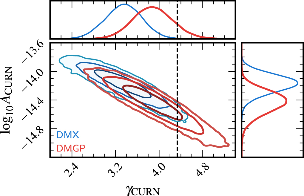
Figure 18. Distribution of real-data and replicated MCOS monopole S/Ns. Each point represents a draw
η
(k) from hd
13/3 posterior, which is used to simulate  and to compute both S/Ns. The replicated monopole S/N is greater for 11% of the simulations.
Download figure:
Standard image High-resolution image
Footnotes
- 74
See Jenet et al. (2006) for an early example of a cross-correlation statistic for PTA GWB detection.
- 75
While the time between the first and last observations we analyze is 16.03 yr, this data set is named "15 yr data set" since no single pulsar exceeds 16 yr of observation; we will use this nomenclature despite the discrepancy.
- 76
The data set is available at http://data.nanograv.org with the code used to process it.
- 77
Throughout the paper we use "red noise" to describe noise whose power spectrum decreases with increasing frequency.
- 78
See Appendix B for details about our Bayesian methods, including the calculation of Bayes factors.
- 79
A Bayesian method for fitting correlations using Legendre polynomials can be found in Nay et al. (2023).