


Abstract
We present the first Event Horizon Telescope (EHT) observations of Sagittarius A* (Sgr A*), the Galactic center source associated with a supermassive black hole. These observations were conducted in 2017 using a global interferometric array of eight telescopes operating at a wavelength of λ = 1.3 mm. The EHT data resolve a compact emission region with intrahour variability. A variety of imaging and modeling analyses all support an image that is dominated by a bright, thick ring with a diameter of 51.8 ± 2.3 μas (68% credible interval). The ring has modest azimuthal brightness asymmetry and a comparatively dim interior. Using a large suite of numerical simulations, we demonstrate that the EHT images of Sgr A* are consistent with the expected appearance of a Kerr black hole with mass ∼4 × 10⁶ M⊙, which is inferred to exist at this location based on previous infrared observations of individual stellar orbits, as well as maser proper-motion studies. Our model comparisons disfavor scenarios where the black hole is viewed at high inclination (i > 50°), as well as nonspinning black holes and those with retrograde accretion disks. Our results provide direct evidence for the presence of a supermassive black hole at the center of the Milky Way, and for the first time we connect the predictions from dynamical measurements of stellar orbits on scales of 103–105 gravitational radii to event-horizon-scale images and variability. Furthermore, a comparison with the EHT results for the supermassive black hole M87* shows consistency with the predictions of general relativity spanning over three orders of magnitude in central mass.
Export citation and abstract BibTeX RIS

Original content from this work may be used under the terms of the Creative Commons Attribution 4.0 licence. Any further distribution of this work must maintain attribution to the author(s) and the title of the work, journal citation and DOI.
1. Introduction
Black holes are among the boldest and most profound predictions of Einstein's theory of general relativity (GR; Einstein 1915). Originally studied as a mathematical consequence of GR rather than as physically relevant objects (Schwarzschild 1916), they are now believed to be generic and sometimes inevitable outcomes of gravitational collapse (Oppenheimer & Snyder 1939; Penrose 1965). In GR, the spacetime around astrophysical black holes is predicted to be uniquely described by the Kerr metric, which is entirely specified by the black hole's mass and angular momentum or "spin" (Kerr 1963).
The first empirical evidence for their existence was through stellar-mass black holes, beginning with observations of X-ray binary orbits (Bolton 1972; Webster & Murdin 1972; McClintock & Remillard 1986) and culminating in the detection of gravitational waves from merging stellar-mass black holes (Abbott et al. 2016). In parallel, the discovery that quasars are not stellar in nature but are rather extremely luminous, compact objects located in the centers of distant galaxies (Schmidt 1963) led to an intensive effort to identify and measure the supermassive black holes (SMBHs) energetically favored to power them (Lynden-Bell 1969). Observations now suggest that SMBHs not only lie at the center of nearly every galaxy (Richstone et al. 1998) but also may play a role in their evolution (see, e.g., Magorrian et al. 1998; Fabian 2012; Kormendy & Ho 2013), though how exactly the ebbs and flows of black hole activity and growth proceed is a major outstanding question in the field.
With the advent of the Event Horizon Telescope (EHT), SMBHs can now be studied with direct imaging (Event Horizon Telescope Collaboration et al. 2019a, 2019b, 2019c, 2019d, 2019e, 2019f, 2021a, 2021b, hereafter M87* Papers I–VIII). The combination of an event horizon and strong lensing near black holes is predicted to produce distinctive gravitational signatures in their images (e.g., Hilbert 1917; Bardeen 1973; Luminet 1979; Jaroszynski & Kurpiewski 1997; Falcke et al. 2000). In particular, simulated images of black holes typically have a central brightness depression encircled by a bright emission ring. The ring usually lies near the gravitationally lensed photon orbits that define the boundary of what we hereafter refer to as the black hole "shadow." The shadow has an angular diameter dsh ≈ 10GM/(c2 D) ≡ 10θ g , where G is the gravitational constant, c is the speed of light, M is the black hole mass, and D is the black hole distance.
From the first realization that SMBHs could power bright radio cores in many galactic nuclei (Lynden-Bell 1969, and references therein), the search has been on to identify them. Within our own Galaxy, the compact source Sgr A* has been intensely studied as a candidate SMBH since its discovery as a bright source of radio emission located near the Galactic center (Balick & Brown 1974; Ekers et al. 1975; Lo et al. 1975). Decades of monitoring its proper motion, as well as motions of individual stars in orbit around it, have revealed Sgr A* to be an extremely dense concentration of mass (M ≈ 4 × 10⁶ M⊙) that is located at and nearly motionless with respect to the dynamical center of the Galaxy (D ≈ 8 kpc), providing strong evidence that it is the nuclear SMBH in our Galaxy (e.g., Do et al. 2019; Gravity Collaboration et al. 2019; Reid & Brunthaler 2020). As the nearest SMBH, Sgr A* provides a unique opportunity to directly image such an object, together with its accretion system, in the most common, quiescent state of SMBHs across the universe. It also provides the chance to elucidate some of the drivers of observed cycles in accretion power and jet launching, via comparison with the more "active" galactic nucleus M87*.
In this paper, we present the first EHT observations of Sgr A* and put them into context with our previous results on M87*. In Section 2, we describe what was previously known about the physical properties of Sgr A* and compare them to M87*. We then summarize our Sgr A* observations with the EHT and other observatories in Section 3 and discuss its variability in Section 4. In Section 5, we present the first EHT images of Sgr A* and analyze its event-horizon-scale structure. In Section 6 we discuss the astrophysical interpretation of these results using an extensive suite of general relativistic magnetohydrodynamic (GRMHD) simulations, and in Section 7 we present the constraints that these results give for GR and black hole alternatives. We provide the overall conclusions and outlook in Section 8. The five companion papers of this series provide a more comprehensive discussion of all these topics (Event Horizon Telescope Collaboration et al. 2022a, 2022b, 2022c, 2022d, 2022e, hereafter Papers II–VI).
2. Sgr A* and M87*
Decades of observations have provided a picture of our local SMBH that is unmatched in any other galaxy (for details about the full spectrum, see Paper II). Sgr A* has been detected from long radio wavelengths (∼1 m) to the hard X-ray band, excepting approximately 1 μm to 1 nm owing to extinction from dust in the Galactic plane. Sgr A* is remarkable for its feeble emission, producing a bolometric luminosity of ≲1036 erg s−1, only ∼100 times that of the Sun. Were it located in another galaxy, it would likely go undetected. Nevertheless, by observing its spectrum and variability, its environment, and its influence on surrounding bodies, a great deal has been learned about this source specifically and about the astrophysical processes that operate around SMBHs. In this section we describe how we assembled our current knowledge of Sgr A*, discuss important theoretical uncertainties about its accretion and outflows, and compare it with the other horizon-scale EHT target, M87*.
2.1. Properties of Sgr A*
The proximity of Sgr A* permits precise measurements of its gravitating mass via the monitoring of resolved individual stellar orbits. High-resolution infrared (IR) observations, using increasingly sophisticated instrumentation and analyses, have traced out the three-dimensional orbits of several stars within the innermost arcsecond around Sgr A* (Schödel et al. 2002; Ghez et al. 2003, 2008; Gillessen et al. 2009; Gravity Collaboration et al. 2018a; Do et al. 2019; Gravity Collaboration et al. 2019). These orbits jointly determine the mass and distance to Sgr A* to high precision, particularly the ratio M/D that determines the angular size of the black hole on the sky. As discussed in Paper II and Paper VI, the current values for the mass and distance suggest an angular shadow diameter close to 50 μas, comparable to that of M87*. The closest orbital periapses confine the mass to within ∼1,000 Schwarzschild radii (RS = 2GM/c2).
Radio observations of SgrA* have provided a significant motivation for the development of the EHT experiment. SgrA* shows a flat/inverted radio spectrum, which often arises from compact jet emission (Blandford & Königl 1979) in other low-luminosity active galactic nuclei (LLAGNs; Ho 1999; Nagar et al. 2000). Such a spectrum can, however, result from any stratified, self-absorbed synchrotron source, where successively higher frequencies are produced at increasingly smaller scales, even without a jet (e.g., Narayan et al. 1995). SgrA* shows an excess of millimeter emission above the flat centimeter-wave spectrum, the so-called "submillimeter bump," that was inferred to indicate the presence of a very compact emitting region at these wavelengths (e.g., Zylka et al. 1992; Falcke et al. 1998).
To clarify the nature of this source, the structure of Sgr A* was investigated using very long baseline interferometry (VLBI) at progressively shorter wavelengths (see Paper II, and references therein). For wavelengths longer than several centimeters, the observed source size is entirely determined by scatter broadening in the ionized interstellar medium, scaling with a wavelength dependence of λ2. At wavelengths of 7 mm and shorter, the imprint of the intrinsic structure of Sgr A* became discernible through the scattering (e.g., Rogers et al. 1994; Lo et al. 1998; Doeleman et al. 2001; Bower et al. 2004; Shen et al. 2005; Bower et al. 2006). The source grows more compact at shorter wavelengths, as expected (e.g., Özel et al. 2000), though it does not present a clear jet structure. For wavelengths as short as ∼1 mm, Sgr A* is only slightly blurred by scattering, and Falcke et al. (2000) predicted that submillimeter VLBI could directly image a brightness depression within this region related to the black hole shadow.
In parallel with these developments and motivated by the goal to study black holes, the capabilities of mm-VLBI improved rapidly. At 1.4 mm, Padin et al. (1990) reported the first VLBI fringes and Krichbaum et al. (1998) obtained the first VLBI detections and associated source size measurements for Sgr A*, each using a two-element interferometer. Doeleman et al. (2008) observed Sgr A* at 1.3 mm with a three-element VLBI array and reported the discovery of an intrinsic source size comparable to the expected angular diameter of the black hole shadow. These observations provided important constraints for theoretical models (e.g., Broderick et al. 2009; Dexter et al. 2009; Mościbrodzka et al. 2009) and strongly suggested that 1.3 mm VLBI has a clear view into the innermost region around the Sgr A* black hole. Subsequent VLBI studies of Sgr A* at 1.3 mm with progressively enhanced arrays revealed the compact emission to be variable and significantly polarized, with measured "closure phases" that are indicative of persistent asymmetry in the image structure (Fish et al. 2011; Johnson et al. 2015; Lu et al. 2018).
Observations of Sgr A* outside the radio band were important for completing the picture of this source as an LLAGN. When X-ray and gamma-ray instruments ROSAT and Sigma/GRANAT (Goldwurm et al. 1994; Predehl & Truemper 1994) could not identify a bright central source, it became clear that Sgr A* must be either obscured or anomalously faint compared to other known LLAGNs. The first identification of Sgr A* as a compact and variable source in the X-rays was achieved with the Chandra X-ray Observatory (Baganoff et al. 2001, 2003). This detection, together with the ∼ 4 × 10⁶ M⊙ mass of Sgr A* determined from stellar orbits, sets a maximum luminosity scale for the source, the so-called Eddington luminosity, 177 and the X-ray measurements confirmed that Sgr A* is approximately 9 orders magnitude less luminous than its LEdd—the lowest Eddington ratio (L/LEdd) observed for any black hole.
This particularly faint high-energy emission stimulated a lively debate regarding the nature of Sgr A*'s accretion/outflow properties and motivated new theoretical developments. If the emission primarily originates in the accretion inflow, either it must be exceptionally radiatively inefficient (Narayan et al. 1995), or the accretion rate onto the black hole must be very small compared to what is captured, or possibly some combination of the two (Blandford & Begelman 1999; Narayan et al. 2000; Quataert & Gruzinov 2000a; Yuan & Narayan 2014). Alternately, the emission could be dominated by an outflow, in which case a small accretion rate would also be favored (Falcke et al. 1993), even during flares (Markoff et al. 2001). Fortunately, the proximity of Sgr A* enables unparalleled study of the accretion flow. Observations with Chandra marginally resolve thermal bremsstrahlung emission from near the gas capture radius, leading to an estimate of the captured accretion rate of ∼ 10−6–10−5 M⊙ yr−1 at ∼ 105 RS (Quataert 2002; Baganoff et al. 2003). The source of this gas can be connected to the observable stellar winds of ∼ 30 individual massive stars found in the inner parsec (Coker et al. 1999; Russell et al. 2017; Ressler et al. 2020). The near-horizon accretion rate has also been estimated to be 10−9–10−7 M⊙ yr−1 through measurements of the Faraday rotation of polarized millimeter emission from Sgr A* (Bower et al. 2003; Marrone et al. 2006, 2007). This Faraday rotation is orders of magnitude smaller than would be expected if the accretion rate at the gas capture radius persisted to small radii (Bower et al. 1999; Agol 2000; Quataert & Gruzinov 2000b; Marrone et al. 2006). This conclusion is further supported by radially resolved X-ray spectroscopy (Wang et al. 2013), suggesting that only ∼ 1% of the captured mass makes it to the SMBH. Taken together, the low luminosity, low radiative efficiency, and weak Faraday rotation are consistent with a weakly bound, magnetized accretion flow so diffuse that the electron and ion temperatures are unable to remain strongly coupled.
Finally, Sgr A* exhibits flaring emission at most wavelengths, including continuous variability at millimeter wavelengths. In particular, approximately daily flares are observed at X-ray and NIR wavelengths that are often (but not always) simultaneous (e.g., Eckart et al. 2004) and that change on timescales as short as minutes (e.g., Baganoff et al. 2001; Genzel et al. 2003). These timescales suggest an origin from within ∼ 5RS of the SMBH, which is consistent with astrometry of NIR flares using the GRAVITY instrument on the Very Large Telescope Interferometer (Gravity Collaboration et al. 2018b).
2.2. Comparison to M87*
M87* and Sgr A* have the largest angular sizes of any known SMBHs, making them the primary EHT targets. However, they differ in several important ways. First, they have substantially different luminosities and accretion rates, both in absolute terms and when scaled by mass. M87*, roughly 1500 × more massive (M = (6.5 ± 0.7) × 109
M⊙; M87* I), has an inferred accretion rate of  and a bolometric luminosity of Lbol ≈ 1042 erg s−1 measured in 2017 (EHT MWL Science Working Group et al. 2021). Estimates of the total kinetic power are typically ∼10–100 times larger, thus conservatively L/LEdd ≳ 10−5 (M87* Paper VIII). Most likely this higher power indicates that M87* is being fed directly from a larger reservoir of gas rather than a trickle from stellar winds. This difference may underlie another substantial divergence between the sources: the prominent, powerful jet launched from M87*, which can be traced at multiple wavelengths and across nearly eight orders of magnitude in size (EHT MWL Science Working Group et al. 2021). The M87* jet provides firm constraints on the source orientation with respect to the line of sight; thus, an inclination of ∼20° was used for numerical simulations in M87* Paper V, while for Sgr A* we do not have any such constraints.
The difference in the masses of Sgr A* and M87* implies a similar difference in their variability timescales. The period of the innermost stable circular orbit (ISCO), which depends on the mass and spin of the black hole, serves as an approximate dynamical timescale. For prograde orbits, this period ranges from 4π
t
g
(maximal spin) to  (zero spin), where t
g
≡ GM/c3. For M87*, this range corresponds to 5 days to 1 month, so the source structure is expected to be effectively unchanged over the course of an observing night. Indeed, EHT images of M87* reconstructed on consecutive nights are almost identical (M87* Paper IV). However, for Sgr A*, the range is only 4–30 minutes, so the source structure can evolve within a single night.
(zero spin), where t
g
≡ GM/c3. For M87*, this range corresponds to 5 days to 1 month, so the source structure is expected to be effectively unchanged over the course of an observing night. Indeed, EHT images of M87* reconstructed on consecutive nights are almost identical (M87* Paper IV). However, for Sgr A*, the range is only 4–30 minutes, so the source structure can evolve within a single night.
3. EHT Observations and Data Processing
In this section we summarize the EHT observations and data processing for Sgr A*. We refer the reader to M87* Paper II for a comprehensive discussion of the EHT instrument, M87* Paper III for details on the 2017 observing campaign and data processing, and Paper II for additional details specific to the Sgr A* data processing.
In 2017, the EHT observed Sgr A* on five nights between April 5 and 11 using an array with eight participating observatories (see Figure 1). Weather conditions were good or excellent at all sites on all five observing nights. The most sensitive element in the array, the Atacama Large Millimeter/submillimeter Array (ALMA), only observed Sgr A* on April 6, 7, and 11; the IRAM 30 m Telescope (PV) only observed Sgr A* on April 7. In this initial series of papers, we focus on the observation with the best baseline coverage: April 7. In addition, we utilize the April 6 observations for testing, validation, and selected multiday analyses. Our multiwavelength coverage indicated that there was an X-ray flare on April 11, accompanied by increased 1.3 mm variability; we will consider that more complex data set in future work.
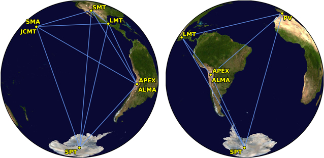
Figure 1. The 2017 EHT array as seen from Sgr A*. The array included eight observatories at six locations: the Atacama Large Millimeter/submillimeter Array (ALMA) and the Atacama Pathfinder Experiment (APEX) on the Llano de Chajnantor in Chile, the Large Millimeter Telescope Alfonso Serrano (LMT) on Volcán Sierra Negra in Mexico, the James Clerk Maxwell Telescope (JCMT) and Submillimeter Array (SMA) on Maunakea in Hawai'i, the Institut de Radioastronomie Millimétrique 30 m telescope (PV) on Pico Veleta in Spain, the Submillimeter Telescope (SMT) on Mt. Graham in Arizona, and the South Pole Telescope (SPT) in Antarctica.
Download figure:
Standard image High-resolution imageEach site, except the JCMT and ALMA, received data in two circular polarizations simultaneously. The JCMT received a single circular polarization, and ALMA received orthogonal linear polarizations that are converted to a circular basis in post-processing. All EHT sites recorded data in two frequency bands at 227.1 and 229.1 GHz, referred to as the "low" and "high" bands, respectively. The total recording rate at each fully outfitted station is 32 GB s–1. The data were written to arrays of hard drives at each site, which were then brought from all sites to common locations where we computed the complex cross-correlation in the electric fields measured for each pair of stations.
Following the initial computation of these correlations, residual phase and bandpass errors were corrected with two independent processing pipelines, EHT-HOPS (Blackburn et al. 2019) and rPICARD (Janssen et al. 2019). The data were then a priori calibrated using the system equivalent flux densities (SEFDs) for each telescope. Multiplication by the geometric mean of the SEFDs of the two stations on a given baseline converts dimensionless correlation coefficients to flux densities. SEFDs ranged from 60 Jy at ALMA to 5 × 10⁴ Jy at low elevation at SMT. Further corrections are still required, as some sites do not measure the SEFD continuously, and in any case the SEFD does not capture many amplitude-corrupting effects such as pointing and focus errors. A "network calibration" process, which uses redundancies in the array (e.g., colocated telescopes) to provide more accurate time-variable gain normalization for sites with colocated partners, was performed. Sgr A* presents a special case for calibration, as it varies significantly in time and is surrounded by extended emission that corrupts the visibility amplitude for baselines within local arrays like ALMA and SMA. Wielgus et al. (2022) discuss the techniques used to estimate the time-resolved flux density of Sgr A* for this calibration. For the remaining stations, gain corrections were computed using observations of the calibrator targets J1924–2914 and NRAO 530 (Paper II).
Figure 2 shows the EHT baseline coverage and interferometric visibility amplitudes ("visibilities") for Sgr A*. The longest baselines have an interferometric fringe spacing of 1/∣ u ∣ ≈ 24 μas, which defines the diffraction-limited angular resolution of the EHT. The visibility amplitudes have two deep minima, the first at ∣ u ∣ ≈ 3.0 Gλ and the second at ∣ u ∣ ≈ 6.5 Gλ. The amplitudes have a baseline dependence that is similar to that of an infinitesimally thin ring with a 54 μas diameter that has been blurred with a circular Gaussian kernel with 23 μas FWHM. The ring diameter is primarily constrained by the minima locations, while the width is determined by the amplitude of the secondary visibility peak between the minima. For instance, to be consistent with both a first minimum falling between 2.5 and 3.5 Gλ and a second minimum falling between 6 and 7 Gλ, the ring must have a diameter of ∼50–60 μas.
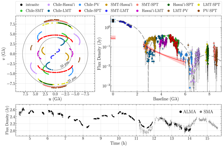
Figure 2. EHT observations of Sgr A* on April 7. Top left: EHT baseline coverage, where dimensionless coordinates u = (u, v) give the projected baseline vector for each antenna pair in units of the observing wavelength λ. Top right: calibrated visibility amplitudes of Sgr A* as a function of projected baseline length ∣ u ∣. Error bars show ±1σ thermal (statistical) uncertainties. Diamonds denote baselines to APEX and JCMT to distinguish them from baselines to their colocated observatories, ALMA and SMA, respectively. The visibilities have been coherently averaged in 120 s intervals. For comparison, the gray dashed line shows the Fourier transform of a thin ring with diameter 54 μas that has been convolved with a circular Gaussian kernel of FWHM 23 μas. The red line and shaded region show the rms variability and associated 68% credible interval over the range of baselines for which it can be accurately measured (see Paper IV), while the blue horizontal ticks at zero baseline length show the range of variations in the total flux density. Bottom: the full light curve of Sgr A* on April 7, measured using ALMA and the SMA as stand-alone interferometers.
Download figure:
Standard image High-resolution imageHowever, the EHT data show evidence for complex and asymmetric source structure beyond a simple ring model, including a strong dependence on visibility amplitudes with the baseline position angle (especially near the first visibility minimum) and in the closure phases measured on triangles of EHT baselines, which differ significantly from 0° and 180°. The EHT visibility amplitudes also show indications of residual calibration errors. To assess and quantify the source morphology of Sgr A* more generally, we applied a variety of imaging and modeling methods using both the interferometric visibility amplitude and phase information (Section 5). These methods included a variety of approaches to account for residual calibration errors, including iterative self-calibration, simultaneous fitting of a model and the residual station gains, and analyses that used only closure quantities.
4. Horizon-scale Variability in Sgr A*
To characterize the spectrum and variability of Sgr A*, the EHT observing campaign was supported by parallel observations at several other observatories. Longer-wavelength VLBI observations, where interstellar scattering prevents direct observation of structural changes, were arranged to occur within a few days of the EHT campaign. IR and X-ray observations were arranged to be as simultaneous as possible with the EHT tracks on several days, and they resulted in one confirmed X-ray flare on April 11.
For the observations of April 6 and 7, when no strong flares were observed in the parallel observations, we must evaluate whether Sgr A* has structural variations within our observation periods. The simplest evidence for variability at λ = 1.3 mm comes from analysis of the total flux density (the "light curve"), which is measured during EHT observations using the ALMA and SMA connected element arrays. As discussed in Wielgus et al. (2022), the fractional variability across all days is approximately 9%, with variations of 4%–13% seen within individual nights (see, e.g., Figure 2). This variability is an order of magnitude stronger than is expected from interstellar scintillation. Thus, the light curves provide evidence for intrinsic image variability in Sgr A*.
Each EHT baseline provides information about the detailed structure of this variability on an angular scale determined by the baseline length. On several triangles, EHT closure phases show slightly more variation than is expected from their thermal noise, the changing of projected baselines (from the source view) with Earth rotation, and interstellar scintillation (Paper II). Comparison of interferometric visibility amplitudes for nearby baselines also reveals variability that significantly exceeds what is expected from thermal noise, calibration uncertainties, and baseline evolution (Paper IV).
To quantify the variability, we developed a simple parametric model for the spatiotemporal power spectrum for the variability of Sgr A* (Georgiev et al. 2022). This model represents the variance in the visibility amplitude as a function of the radial distance in the (u, v)-plane, taking the form of a broken power law, as motivated by studies of GRMHD simulations. The source-integrated light curve is divided out in order to isolate structural variation from overall changes in flux density. The variability power spectrum was also empirically estimated by analyzing variations in visibility amplitudes on nearby baselines (Broderick et al. 2022). This comparison included the same baselines sampled on different days, as well as nearby or crossing baseline tracks (e.g., SPT-LMT and SPT-SMA sample nearly identical baselines, but at different times). This analysis revealed that the fractional variability can be order unity for EHT baselines located near the two deep visibility minima (Figure 2), even after normalizing the data to remove light-curve fluctuations, and that it significantly exceeds the variability expected from interstellar scintillation (Paper IV).
5. Horizon-scale Structure in Sgr A*
Each interferometric visibility samples a single complex Fourier component of the image on the sky (e.g., Thompson et al. 2017). Interferometric imaging algorithms seek to produce images from this sparse Fourier-domain information that are consistent with the data and physically plausible. Techniques such as the classical CLEAN algorithm and regularized maximum likelihood (RML) methods successfully produced EHT images of M87*, with remarkable agreement among methods (M87* Paper IV). The EHT baseline coverage for Sgr A* is substantially better than for M87*, primarily because of the additional telescope (SPT) with mutual visibility of the source. Moreover, at λ = 1.3 mm, Sgr A* has a compact flux density that is approximately four times larger than that of M87*, with no appreciable contribution to the short-baseline visibilities from an extended jet. However, producing an image of Sgr A* requires additional assumptions because of the rapid source variability and interstellar scattering.
Specifically, VLBI imaging typically relies on Earth-rotation aperture synthesis, in which the projection of each baseline sweeps out an arc in the (u, v)-plane as the Earth rotates, allowing a sparse array of telescopes to obtain the (u, v)-coverage necessary for the imaging of a static source (Thompson et al. 2017). To account for the source structural variability, we used a parametric model discussed in Section 4. By incorporating this variability error budget, imaging and modeling methods designed for a static source can be applied to analyze data from a variable source.
To account for the interstellar scattering, we used two approaches (Paper III). The first, "on-sky imaging," applies no modifications to the data or images. In this approach, the algorithms simply reconstruct the scattered image of the source. The second, "descattered imaging," adds an error budget to interferometric visibilities to account for stochastic scattering substructure before deconvolving the ensemble-average scattering kernel. Both the ensemble-average kernel and the power spectrum of scattering are used (Psaltis et al. 2018), each of which is precisely known from an analysis combining decades of observations of Sgr A* at centimeter wavelengths (Johnson et al. 2018).
To test these imaging techniques and to select appropriate imaging parameters, we developed a suite of synthetic observations of seven geometric models that share the scattering and variability properties of Sgr A*. This suite included models with widely varying morphologies: rings, disks, a crescent, a double source, and a point-like source with an extended halo. Each model was selected to produce visibility amplitudes that were similar to those of Sgr A*, with two deep visibility minima, a physical scattering model applied, and stochastic temporal evolution generated by a statistical model (Lee & Gammie 2021).
We then selected the sets of imaging parameters that accurately reconstruct images across the entire test suite, including both ring and nonring data sets. These "top set" parameter choices yield a corresponding collection of reconstructed images of Sgr A* that provide both a representative average image and a measure of its uncertainty. In addition, we used a new Bayesian imaging method, which simultaneously estimates both the reconstructed image and its associated variability noise model (Broderick et al. 2020). This method does not require training on synthetic data, although we used the same test suite for comparison and validation of this method.
When applied to the Sgr A* data, over 95% of the top set images have a prominent ring morphology. For an analysis using the combination of April 6 and 7 data, all samples from the Bayesian imaging posterior show a ring morphology. In addition, geometric modeling of the EHT data shows a consistent statistical preference for ring morphologies over alternatives with comparable complexity. The ring has a diameter, width, and central brightness depression that are consistent across the different choices of imaging methods and parameters (see Paper III). However, the reconstructed images show diversity in their specific attributes, particularly the azimuthal intensity distribution around the ring. This uncertainty is a consequence of the limited EHT baseline coverage, compounded by the challenges of imaging a variable source. We categorized the reconstructed images into four clusters spanning the primary reconstructed structures: three clusters are ring modes with varying position angle, while the fourth is a comparatively small set of reconstructed images with diverse nonring morphologies. Figure 3 shows a representative average image of Sgr A* on April 7, as well as the average image for each of these clusters along with their relative occurrence frequency.

Figure 3. Representative EHT image of Sgr A* from observations on 2017 April 7. This image is an average over different reconstruction methodologies (CLEAN, RML, and Bayesian) and reconstructed morphologies. Color denotes the specific intensity, shown in units of brightness temperature. The inset circle shows the restoring beam used for CLEAN image reconstructions (20 μas FWHM). The bottom panels show average images within subsets with similar morphologies, with their prevalence indicated by the inset bars. The multiplicity of image modes reflects uncertainty due to the sparse baseline coverage; it does not correspond to different snapshots of the variable source. Nearly all reconstructed images show a prominent ring morphology. While the diameter and thickness of the ring are generally consistent across the reconstructions, the azimuthal structure of the ring is poorly constrained.
Download figure:
Standard image High-resolution imageTo quantify the ring parameters in a complementary way, we used several geometrical modeling methods, the parameterizations of which were guided by the reconstructed images of Sgr A*. These models are defined by a thick ring with azimuthal variations determined by low-order Fourier coefficients and an additional Gaussian brightness floor. Because these simple geometric models have a small number of parameters, they can be constrained using instantaneous snapshots of data. Hence, we used two modeling approaches. With "snapshot" modeling, we aggregate a series of independent fits to 2-minute data segments. This approach does not require a variability model. With "full-track" modeling, we fit both a static geometric source model and a variability noise model simultaneously to the entire 12 hr observation. Table 1 summarizes the consensus ring parameters measured using these methods (for detailed results from individual methods, see Paper IV).
Table 1. Measured Parameters of Sgr A*
| Parameter | EHT Estimate |
|---|---|
| Emission ring: a | |
| Diameter, d | 51.8 ± 2.3 μas |
| Fractional width, W/d | ∼30–50 |
| Orientation, η | ⋯ |
| Brightness asymmetry, A | ∼0.04–0.3 |
| Angular gravitational radius, a θ g |

|
| Black hole mass, b M |

|
| Angular shadow diameter, c dsh | 48.7 ± 7.0 μas |
| Schwarzschild shadow deviation, c δ |
 (VLTI) (VLTI) |
 (Keck) (Keck) | |
| Parameter | Previous Estimate |
| Angular gravitational radius, θ g : | |
| Stellar orbits (VLTI) d | 5.125 ± 0.009 ± 0.020 μas |
| Stellar orbits (Keck) e | 4.92 ± 0.03 ± 0.01 μas |
| Black hole distance, D: | |
| Stellar orbits (VLTI) d | 8277 ± 9 ± 33 pc |
| Stellar orbits (Keck) e | 7935 ± 50 ± 32 pc |
| Masers (cm VLBI) | 8150 ± 150 pc |
| Black hole mass, M: | |
| Stellar orbits (VLTI) d | (4.297 ± 0.013) × 106 M⊙ |
| Stellar orbits (Keck) e | (3.951 ± 0.047) × 106 M⊙ |
Notes.
a The orientation and magnitude of the ring's brightness asymmetry are poorly constrained; they vary significantly among the reconstructed image modes and among different modeling and imaging methods. For details, see Paper IV. b To translate our estimate of θ g into an estimated mass of Sgr A*, we use the distance to Sgr A* estimated using trigonometric VLBI parallaxes and proper motions of molecular masers in spiral arms of the Milky Way (Reid et al. 2019). For details, see Paper IV. c Estimates of dsh are determined solely from EHT data, but estimates of δ use priors for θ g from resolved stellar orbits as indicated. For details, see Paper VI. d Gravity Collaboration et al. (2022). e Do et al. (2019). f Reid et al. (2019).Download table as: ASCIITypeset image
In Paper III, we also used dynamic imaging and snapshot ring modeling to analyze the intraday image variability in Sgr A*. We applied these analysis methods to the 100-minute intervals on April 6 and 7 with the best sampling (Farah et al. 2022), adopting a strong ring prior to counteract the limited baseline coverage. On April 6, most dynamic imaging and modeling methods recover a nearly static image, while many reconstructions on April 7 find an evolving image. However, the results on April 7 are strongly affected by the underlying prior assumptions; different parameters in the dynamic imaging method result in different modes of position angle evolution in the reconstructed images, including some reconstructions that are nearly static. Thus, while the EHT data show detectable signs of image variability, we cannot reliably constrain the underlying image evolution.
6. Implications for Accretion and Outflow Physics
What can we learn from these images and their variability properties? Focusing first on the astrophysics of the accretion process and jet launching, we can explore which physical scenarios are most consistent with our results, under the assumption that Sgr A* is a Kerr black hole with mass and distance accurately determined from stellar orbits. Our constraints on the properties of the black hole and potential deviations from GR are explored in Section 7.
We assume that the accretion structure around Sgr A* is approximately governed by ideal GRMHD, as was done for M87*, which is common in the literature for modeling SMBHs (see, e.g., Gammie et al. 2003). Decades of observations and semianalytical modeling (see Paper V for details, references, and caveats) constrain the average plasma properties close to the event horizon of Sgr A*, allowing us to make several additional simplifying approximations. In particular, for Sgr A* we can assume that radiative cooling does not strongly affect the dynamics and that the electrons and ions are weakly coupled by Coulomb collisions, so that ions and electrons can have distinct temperatures in some parts of the flow.
Because we model the plasma as a fluid with a single temperature, one of our main sources of uncertainty is the treatment of the electrons, whose presence is not explicitly accounted for in the simulation evolution equations. We explore several parameterized models to assign the electron distribution function (eDF), assuming that the electron temperature is proportional to the proton temperature, with a proportionality that depends on the ratio of gas to magnetic pressure (Chan et al. 2015). The eDFs include thermal and nonthermal variations, the latter of which were not explored in the M87* 2017 papers. Our fiducial thermal models employ the same eDF prescription as for the M87* papers, using only one free parameter, Rhigh, to specify the proton-to-electron temperature ratio in regions where gas pressure dominates the magnetic pressure (Mościbrodzka et al. 2016). This ratio is typically larger in the disk midplane than in the jet/outflow. Since the radiation is produced by electrons, increasing Rhigh effectively increases the brightness of the jets/outflow region relative to the disk and changes the resulting images/spectra (M87* Paper V). Compared to M87*, we also allow the inclination angle to vary.
We employ five different ideal GRMHD codes to explore a large swath of overlapping parameter space, in some cases with very similar setups allowing for consistency checks. In other cases, with a more exploratory sampling of parameter space, we also allow differences in, for example, adiabatic index, resolution, and size of the tori and/or computational domain. Most models are initialized with an orbiting torus of plasma with characteristic radius ∼20G M/c2. The torus is seeded with a weak, poloidal magnetic field and can be either prograde or retrograde with respect to the black hole spin (a free parameter). We also consider a limited set of exploratory models, such as those with "tilt" where the black hole spin axis is misaligned from the rotation axis of the torus (Liska et al. 2018; Chatterjee et al. 2020; White & Quataert 2022), as well as a model initiated on a very large grid using a more realistic setup for the outer boundary conditions in which the accretion flow is directly fed by winds from orbiting stars (Ressler et al. 2020). Both of these are more realistic physical scenarios but also allow a much larger range of parameter space than we could fully explore.
We classify the fiducial models as being in either the magnetically arrested disk (MAD; Narayan et al. 2003) or standard and normal evolution (SANE; Narayan et al. 2012) modes. In MAD models the ordered magnetic fields significantly affect the dynamics of the flow, episodically halting accretion onto the black hole, while SANE models have weaker, more turbulent magnetic fields. Because the dynamical timescale in Sgr A* is short compared to a night of observations, it is important to run each model for enough time to capture the range of spectral and structural variations. The simulations are typically run for 30,000t g , while some are run for more than 100,000t g in order to sample a broader distribution of behavior.
For each time-dependent GRMHD simulation, with an eDF prescription and inclination with respect to the line of sight, we calculate a sequence of model images (movies) using ray-tracing and including synchrotron emission and absorption. We also calculate spectra including synchrotron emission and absorption, bremsstrahlung emission, and, using Monte Carlo methods, Compton scattering. These synthetic data sets are then used to generate simulated EHT images, as well as multiwavelength light curves and spectral energy distributions (SEDs), for comparison with the Sgr A* data described in Paper II. We scale all images to a benchmark average flux density of 2.4 Jy at 230 GHz to match the average synchrotron flux density of Sgr A* (see Paper II; Wielgus et al. 2022).
We evaluate the simulations against three types of observational constraints: EHT interferometric measurements, emission at other wavelengths, and variability. The EHT constraints include (1) a measure of the image size; (2) salient features from the visibility amplitudes, such as the location of the first deep minimum; and (3) the diameter, asymmetry, and width of simplified ring models fitted to well-sampled portions of the April 7 visibility data. The constraints from other wavelengths include the flux densities at 86 GHz, 2.2 μm in the NIR, and X-ray and the major-axis source size at 86 GHz, constrained from observations with the Global mm-VLBI Array. Finally, the variability constraints are (1) the fractional 230 GHz variability on 3 hr timescales, derived from more than a decade of measurements; and (2) the structural variability of the source, calculated at a baseline length of 4Gλ after fitting a parameterized model to the visibility amplitude variation versus baseline length. See Paper V for the full ranges of tests and pass/fail conditions.
Compared to M87* Paper V, we explore a larger range of models and model parameter space, and we also include some additional observational constraints. These include the degree of intrinsic variability and the broadband spectral constraints given above. Accordingly, we find that all our models fail at least one of the observational constraints. These results indicate the power of combining interferometric data with other observational constraints to narrow down the viable physical parameter space. We now summarize our main results and their implications for our understanding of Sgr A*'s accretion state and geometry.
We primarily focus on a set of "fiducial" simulations, which use aligned (prograde or retrograde) accretion flows and thermal eDFs defined via the Rhigh prescription. We declare a model to fully pass a set of constraints only when all GRMHD simulations with those parameters pass. This approach helps to ensure that our selection of favored models is resilient to small variations in the GRMHD simulation choices and software. Figure 4 summarizes these results.
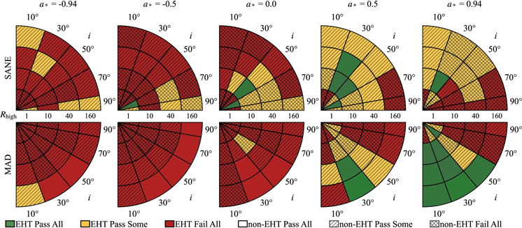
Figure 4. Summary of constraints on our 200 fiducial GRMHD simulations. Color indicates combined EHT constraints apart from structural or flux variability, and hatching indicates combined non-EHT constraints. For each constraint category and parameter combination, we delineate whether all of the three simulation codes run with those parameters pass, whether only some pass, or whether none pass. These exclusions leave only two models, each a MAD with prograde spin, 30° inclination, and Rhigh = 160. For details, see Paper V.
Download figure:
Standard image High-resolution imageAll edge-on (high inclination) models fail the combined set of EHT-only constraints for at least one simulation, and almost all retrograde models (a* < 0) fail. There are two interesting groupings of models that pass all EHT constraints for all simulations: both have positive/prograde spin (a* = 0.5, 0.94) with lower ( ≤ 50°) inclination, but some are MAD (10) and some are SANE (8). With only ∼ 10% pass rate for all models, it is clear that EHT imaging data alone are capable of strongly down-selecting the potential model space. The more heterogeneous non-EHT constraints prefer a rather different set of models. However, even with all these constraints, 11/200 models pass for all simulations; all of these are MADs, with all but one having Rhigh = 160. On the other hand, they cover a wider range of spin compared to EHT-only constraints, with a slight preference for a* ≤ 0 and higher inclinations, and including retrograde and edge-on models.
None of the 200 fiducial models pass all 11 constraints in combination, the most strict of which are the 86 GHz size, the ring diameter, and the light-curve variability on 3 hr timescales. Of these, the light-curve variability turns out to be the most stringent constraint, passing only 4% of fiducial models. SANE models, which are less variable than MADs, are preferred, while all the other EHT/non-EHT constraints generally favor MADs. If we consider the set of models that pass 10/11 constraints, it is notable that for both MADs and SANEs there is still a marked preference for models with prograde spin, a lower inclination, and Rhigh > 40, with several clustered at the maximum of Rhigh = 160.
The "exploratory" models cover less of a range in parameter space but still indicate important trends. In particular, including nonthermal electrons (which are especially important for modeling flares) tends to push the limits of allowed NIR flux and, to some extent, also the X-ray flux. Because the nonthermal particles also enhance the 230 GHz flux density, rescaling to a fixed flux density results in a smaller accretion rate. The smaller resulting opacity then affects the image properties, such as producing a somewhat narrower ring morphology at 230 GHz and a larger image at 86 GHz. Nevertheless, the addition of nonthermal models does not drastically change the preferred parameter space, and passing models also favor prograde spin and lower inclination. Increased tilt of the accretion flow tends to increase variability and the NIR flux and thus leads to model failures. Similarly, neither of the two wind-fed models passed, but this is not surprising, as they only model a single spin (a* = 0) and two instances of the thermal Rhigh eDF. With such sparse sampling of parameter space, these classes of models require a more focused study to draw conclusions.
Overall, very few of our models are as quiet as the data. Although this was not investigated in M87* Paper V, subsequent work suggests a similar result for M87* simulations (Satapathy et al. 2022). In general, SANE models are less variable than MADs, and face-on models are somewhat less variable than edge-on. However, there are limitations of the modeling that may affect the variability. For instance, collisionless effects, radiative cooling, and improved electron heating models could all potentially reduce variability. Thus, our variability constraints may be too strict.
There are only two models that pass everything but the variability constraints. The models have similar parameters: both are MAD, both are prograde spin (one has a* = 0.5, and the other has a* = 0.94), and both have i = 30° and Rhigh = 160. Figure 5 shows a representative snapshot from one of these simulations and its corresponding image reconstruction. If we take these two models as indicative, there is a preference for accretion rates at the lower end of the range found by other constraints, 10−9–10−8 M⊙ yr−1, and an outflow power of ∼ 1038 erg s−1, which is comparable to the bolometric luminosity of stellar-mass black holes in X-ray binaries. The combination of high Rhigh and relatively low inclination satisfies the spectral constraints without their associated jet structure producing too much asymmetry to satisfy the EHT constraints. A low inclination is also consistent with the independent estimate based on tracking the motions of NIR flaring structures using the VLTI (Gravity Collaboration et al. 2018b). Our results highlight the value of continued EHT plus multiwavelength monitoring of Sgr A*, and there is clearly much more exploration to conduct, including improved theoretical models and numerical simulations, full SED modeling, and polarimetric imaging, all of which will yield deeper physical insights (see, e.g., Event Horizon Telescope Collaboration et al. 2021b).
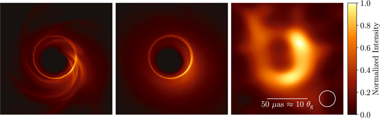
Figure 5. Simulated images of Sgr A*. Left: a single snapshot image of a numerical simulation of Sgr A* that passes 10 out of the 11 observational criteria described in Paper V. Middle: the average of this simulation with time sampling that matches the EHT observational cadence on April 7. Right: representative image reconstruction using synthetic visibilities generated from the simulation in the adjacent panels (see Appendix H in Paper III). This image has been averaged across methodologies and reconstructed morphologies, as in Figure 3. Each panel is shown on a linear brightness scale that is normalized to its peak.
Download figure:
Standard image High-resolution image7. Implications for Black Holes and General Relativity
As demonstrated using the suite of GRMHD simulations discussed in Section 6, the EHT images of Sgr A* are consistent with the expected appearance of a Kerr black hole. Moreover, our images are consistent with an angular gravitational radius θ g that matches the expectations from nearly Keplerian orbits of stars on scales of (103–105)RS.
To quantify this consistency, we compute θ g using EHT measurements alone (for details, see Paper IV). Following the procedure developed in M87* Paper VI, we estimate θ g by calibrating the observed emission ring diameter d to the known angular gravitational scale θ g for a suite of synthetic data sets produced from the GRMHD library presented in Paper V. Specifically, we generate 100 data sets from GRMHD simulations with varying intrinsic θ g and that span the explored range in accretion states, black hole spins, viewing inclinations, position angles, and phenomenological electron heating parameters Rhigh. Each synthetic data set matches the baseline coverage and sensitivity of the EHT observations. We then estimate the ring diameter using multiple geometric modeling and imaging methods, deriving a separate calibration factor α ≡ d/θ g for each method and for every data set to attain a method-dependent scaling relationship and associated uncertainty.
With this approach, we estimate  for Sgr A*, where the uncertainties correspond to a 68% credible interval. This estimate is consistent with, but much less constraining than, measurements of θ
g
using resolved stellar orbits (see Table 1). This procedure assumes the validity of the Kerr metric and relies on our suite of GRMHD simulations to provide a reasonable proxy for the space of viable emission models. The fractional uncertainty in our estimate of θ
g
for Sgr A* is broader than our estimate for M87* (θ
g
= 3.8 ± 0.4 μas), primarily because of the increased calibration uncertainty associated with the unknown inclination of Sgr A* and because of the increased diameter measurement uncertainty associated with intrinsic variability of Sgr A*.
for Sgr A*, where the uncertainties correspond to a 68% credible interval. This estimate is consistent with, but much less constraining than, measurements of θ
g
using resolved stellar orbits (see Table 1). This procedure assumes the validity of the Kerr metric and relies on our suite of GRMHD simulations to provide a reasonable proxy for the space of viable emission models. The fractional uncertainty in our estimate of θ
g
for Sgr A* is broader than our estimate for M87* (θ
g
= 3.8 ± 0.4 μas), primarily because of the increased calibration uncertainty associated with the unknown inclination of Sgr A* and because of the increased diameter measurement uncertainty associated with intrinsic variability of Sgr A*.
We also used EHT images to constrain potential deviations from the Kerr metric and to test the nature of the compact object in Sgr A* (for details, see Paper VI). For instance, the brightness depression has a contrast f
c
≲ 0.3, which provides support for the existence of an event horizon in Sgr A*. If the compact object instead had an absorptive boundary that radiated the thermalized energy of infalling material  , it could still produce a depression in the EHT images but would generate IR emission that greatly exceeds the measured spectrum of Sgr A* (Broderick & Narayan 2006; Narayan & McClintock 2008). Alternatively, a partially reflecting surface would reduce the depth of the depression; the EHT images directly constrain the albedo of such a reflecting surface to be ≲0.3. The brightness depression also rules out several specific black hole alternatives, including some models of naked singularities (e.g., Joshi et al. 2014) and some models of boson stars (e.g., Olivares et al. 2020), although other horizonless black hole mimickers produce apparent shadows that are consistent with the observed depression (e.g., Shaikh et al. 2019).
The measured ring diameter also provides constraints on the spacetime metric. To obtain these constraints, we generate a series of synthetic images to relate a measured emission ring diameter to that of the underlying black hole shadow. These images included a broad range of GRMHD simulations from Paper V, as well as images for which the GRMHD and underlying metric assumptions are relaxed. Specifically, we generated sets of images of analytic models for accretion onto (1) a Kerr black hole, (2) a black hole with parametric deviations from Kerr given by the Johannsen−Psaltis metric (Johannsen & Psaltis 2011), and (3) a non-Kerr black hole defined by the Kerr−Sen metric (García et al. 1995). For each analytic model, we allow the emission prescriptions to vary within physically plausible limits (for details, see Özel et al. 2021; Younsi et al. 2021). We find a similar relationship between the diameter of the emission ring and that of the black hole shadow in all these cases, indicating that this relationship is insensitive to the details of the underlying spacetime.
Selecting a subset of these models, we then generate 145 synthetic data sets. We apply imaging and modeling methods to compute the ring diameter for each data set to evaluate method-dependent measurement uncertainties and biases. We then use this calibration together with the EHT measurements of the ring diameter to determine the angular diameter of the black hole shadow for Sgr A*: dsh = 48.7 ± 7.0 μas. This result is tighter than the range for θ g derived above because of differences in the calibration data sets and procedures used in Paper IV and Paper VI. Specifically, Paper IV uses a calibration suite that consists entirely of dynamic GRMHD models, and it derives a scale factor between θ g and the angular diameter of the emission ring. In contrast, Paper VI uses a calibration suite containing both static Kerr and non-Kerr images and dynamic GRMHD models, and it derives a scale factor between dsh and the angular diameter of the emission ring. Paper VI also excludes data sets for which the range of reconstructed diameters is more than 2–3 times the range that is measured using the Sgr A* data. Thus, comparison of these results provides a measure of the impact of our assumptions and procedures on the inference of the black hole properties.
By comparing this shadow diameter with stellar-dynamical measurements of the mass of Sgr A*, we also determine a deviation parameter δ, which quantifies the fractional difference between the inferred shadow diameter and its expected value for a nonspinning (Schwarzschild) black hole (for details, see Paper VI). We find  when using VLTI measurements of θ
g
and
when using VLTI measurements of θ
g
and  when using Keck measurements of θ
g
(see Table 1). For comparison, a spinning (Kerr) black hole has −0.08 ≤ δ ≤ 0.
when using Keck measurements of θ
g
(see Table 1). For comparison, a spinning (Kerr) black hole has −0.08 ≤ δ ≤ 0.
Under the assumption that this range of calibration factors applies generically to all non-Kerr spacetimes that have black hole shadows, we can translate measurements of δ into constraints on parameters of these spacetimes (Psaltis et al. 2020). In particular, our measurements exclude specific non-Kerr solutions for Sgr A*, such as the traversible Morris−Thorne wormhole and the naked singularities in the Reissner−Nordström metric, which predict shadows that are significantly smaller than those of Kerr black holes.
Relative to M87*, the primary strengths of testing GR with EHT observations of Sgr A* are the tight prior constraints on its mass-to-distance ratio θ g and its shorter gravitational timescale that allows EHT observations to span many dynamical times. Together, these results show SMBHs consistent with predictions of the Kerr metric over a spread of three orders of magnitude in their mass (see Figure 6). The image of Sgr A* probes a similar gravitational potential to M87* but spacetime curvature ξ ∝ M−2 that is six orders of magnitude larger. When combined with constraints from the measurement of gravitational waves from coalescing black hole binaries with LIGO/Virgo, these results show a striking validation of the predictions of GR over a vast range of scales, from stellar-mass black holes to SMBHs that are billions of times larger.

Figure 6. Comparison of posterior distributions for the Schwarzschild fractional shadow deviation parameter δ measured by the EHT for Sgr A* and M87*. For Sgr A*, δ is computed relative to the expected shadow size from monitoring stellar orbits; for M87*, δ is computed for the expected shadow both from stellar dynamics and from gas dynamics (for details, see M87* Paper VI). The gray band shows the expected range of δ for the Kerr metric. For the stellar-dynamical prior mass estimates, the EHT measurements show close consistency with the same black hole metric over three orders of magnitude in black hole mass.
Download figure:
Standard image High-resolution image8. Conclusion and Outlook
Here we present the results of 2017 EHT observations of Sgr A*, the central SMBH in the Milky Way. We find evidence for intraday structural variability in Sgr A*, confirming changes that were hinted at in prior observations across the electromagnetic spectrum. These variations challenge standard approaches to interferometric analysis, so we have developed a variety of methods to infer the structure of this source from our data. From observations on April 7, on which we have the best-sampled data, our analyses consistently reveal a ring-like structure, similar to that seen in M87*. Less complete observations on April 6 support this picture.
This ring of emission and its central brightness depression closely mirror the structure expected from the plasma in accretion and outflow structures bordering the event horizon of a black hole and partially lensed by its gravity. The angular diameter of this ring is consistent with that expected from the black hole mass inferred from stellar orbits. This consistency allows us to restrict the allowed values of parameters that describe deviations from a Kerr black hole, as predicted by GR. We compare our data, including measurements at other wavelengths, with a large suite of GRMHD simulations. These simulations are remarkably successful at predicting the 1.3 mm image structure and broadband spectrum of Sgr A*. However, the GRMHD simulations tend to be more variable than the observations, which may be related to our fluid modeling of a collisionless plasma or our neglect of radiative cooling, and only a few configurations can satisfy our full set of observational constraints apart from variability. Our results generally favor models with dynamically strong magnetic fields, moderate (prograde) spin, a lower inclination viewing angle, and strongly decoupled protons and electrons in the emission region. Interestingly, these models also predict a reasonably efficient (compared to the accretion rate) jet outflow, which points to interesting complementary future studies. However, more work is needed to fully explore the physical parameter space and to understand the variability.
As the nearest SMBH, Sgr A* can be scrutinized in ways that are impossible for other sources, making it a unique laboratory for exploring the astrophysics of black holes and testing the predictions of GR. The results presented in these papers are the first EHT contributions to the study of this source, but they are not the last. Subsequent work will characterize the magnetic field configuration of this source through polarimetric observations, as was done for M87*, and describe the structural changes associated with flare activity on April 11. Since 2017, the EHT has continued to gather data using an increasing number of array elements and doubled recording bandwidth. These data will provide improved sensitivity and enable more robust imaging of this dynamic source, eventually allowing movie reconstructions of plasma motions on the ∼hour orbital timescales.
We thank the anonymous referees for helpful comments that improved the paper.
The Event Horizon Telescope Collaboration thanks the following organizations and programs: the Academia Sinica; the Academy of Finland (projects 274477, 284495, 312496, 315721); the Agencia Nacional de Investigación y Desarrollo (ANID), Chile via NCN19_058 (TITANs) and Fondecyt 1221421, the Alexander von Humboldt Stiftung; an Alfred P. Sloan Research Fellowship; Allegro, the European ALMA Regional Centre node in the Netherlands, the NL astronomy research network NOVA and the astronomy institutes of the University of Amsterdam, Leiden University and Radboud University; the ALMA North America Development Fund; the Black Hole Initiative, which is funded by grants from the John Templeton Foundation and the Gordon and Betty Moore Foundation (although the opinions expressed in this work are those of the author(s) and do not necessarily reflect the views of these Foundations); Chandra DD7-18089X and TM6-17006X; the China Scholarship Council; China Postdoctoral Science Foundation fellowship (2020M671266); Consejo Nacional de Ciencia y Tecnología (CONACYT, Mexico, projects U0004-246083, U0004-259839, F0003-272050, M0037-279006, F0003-281692, 104497, 275201, 263356); the Consejería de Economía, Conocimiento, Empresas y Universidad of the Junta de Andalucía (grant P18-FR-1769), the Consejo Superior de Investigaciones Científicas (grant 2019AEP112); the Delaney Family via the Delaney Family John A. Wheeler Chair at Perimeter Institute; Dirección General de Asuntos del Personal Académico-Universidad Nacional Autónoma de México (DGAPA-UNAM, projects IN112417 and IN112820); the Dutch Organization for Scientific Research (NWO) VICI award (grant 639.043.513) and grant OCENW.KLEIN.113; the Dutch National Supercomputers, Cartesius and Snellius (NWO Grant 2021.013); the EACOA Fellowship awarded by the East Asia Core Observatories Association, which consists of the Academia Sinica Institute of Astronomy and Astrophysics, the National Astronomical Observatory of Japan, Center for Astronomical Mega-Science, Chinese Academy of Sciences, and the Korea Astronomy and Space Science Institute; the European Research Council (ERC) Synergy Grant "BlackHoleCam: Imaging the Event Horizon of Black Holes" (grant 610058); the European Union Horizon 2020 research and innovation programme under grant agreements RadioNet (No 730562) and M2FINDERS (No 101018682); the Generalitat Valenciana postdoctoral grant APOSTD/2018/177 and GenT Program (project CIDEGENT/2018/021); MICINN Research Project PID2019-108995GB-C22; the European Research Council for advanced grant "JETSET: Launching, propagation and emission of relativistic jets from binary mergers and across mass scales" (Grant No. 884631); the Institute for Advanced Study; the Istituto Nazionale di Fisica Nucleare (INFN) sezione di Napoli, iniziative specifiche TEONGRAV; the International Max Planck Research School for Astronomy and Astrophysics at the Universities of Bonn and Cologne; DFG research grant "Jet physics on horizon scales and beyond" (Grant No. FR 4069/2-1); Joint Princeton/Flatiron and Joint Columbia/Flatiron Postdoctoral Fellowships, research at the Flatiron Institute is supported by the Simons Foundation; the Japan Ministry of Education, Culture, Sports, Science and Technology (MEXT; grant JPMXP1020200109); the Japanese Government (Monbukagakusho: MEXT) Scholarship; the Japan Society for the Promotion of Science (JSPS) Grant-in-Aid for JSPS Research Fellowship (JP17J08829); the Joint Institute for Computational Fundamental Science, Japan; the Key Research Program of Frontier Sciences, Chinese Academy of Sciences (CAS, grants QYZDJ-SSW-SLH057, QYZDJSSW-SYS008, ZDBS-LY-SLH011); the Leverhulme Trust Early Career Research Fellowship; the Max-Planck-Gesellschaft (MPG); the Max Planck Partner Group of the MPG and the CAS; the MEXT/JSPS KAKENHI (grants 18KK0090, JP21H01137, JP18H03721, JP18K13594, 18K03709, JP19K14761, 18H01245, 25120007); the Malaysian Fundamental Research Grant Scheme (FRGS) FRGS/1/2019/STG02/UM/02/6; the MIT International Science and Technology Initiatives (MISTI) Funds; the Ministry of Science and Technology (MOST) of Taiwan (103-2119-M-001-010-MY2, 105-2112-M-001-025-MY3, 105-2119-M-001-042, 106-2112-M-001-011, 106-2119-M-001-013, 106-2119-M-001-027, 106-2923-M-001-005, 107-2119-M-001-017, 107-2119-M-001-020, 107-2119-M-001-041, 107-2119-M-110-005, 107-2923-M-001-009, 108-2112-M-001-048, 108-2112-M-001-051, 108-2923-M-001-002, 109-2112-M-001-025, 109-2124-M-001-005, 109-2923-M-001-001, 110-2112-M-003-007-MY2, 110-2112-M-001-033, 110-2124-M-001-007, and 110-2923-M-001-001); the Ministry of Education (MoE) of Taiwan Yushan Young Scholar Program; the Physics Division, National Center for Theoretical Sciences of Taiwan; the National Aeronautics and Space Administration (NASA, Fermi Guest Investigator grant 80NSSC20K1567, NASA Astrophysics Theory Program grant 80NSSC20K0527, NASA NuSTAR award 80NSSC20K0645); NASA Hubble Fellowship grant HST-HF2-51431.001-A awarded by the Space Telescope Science Institute, which is operated by the Association of Universities for Research in Astronomy, Inc., for NASA, under contract NAS5-26555; the National Institute of Natural Sciences (NINS) of Japan; the National Key Research and Development Program of China (grant 2016YFA0400704, 2017YFA0402703, 2016YFA0400702); the National Science Foundation (NSF, grants AST-0096454, AST-0352953, AST-0521233, AST-0705062, AST-0905844, AST-0922984, AST-1126433, AST-1140030, DGE-1144085, AST-1207704, AST-1207730, AST-1207752, MRI-1228509, OPP-1248097, AST-1310896, AST-1440254, AST-1555365, AST-1614868, AST-1615796, AST-1715061, AST-1716327, AST-1716536, OISE-1743747, AST-1816420, AST-1935980, AST-2034306); NSF Astronomy and Astrophysics Postdoctoral Fellowship (AST-1903847); the Natural Science Foundation of China (grants 11650110427, 10625314, 11721303, 11725312, 11873028, 11933007, 11991052, 11991053, 12192220, 12192223); the Natural Sciences and Engineering Research Council of Canada (NSERC, including a Discovery Grant and the NSERC Alexander Graham Bell Canada Graduate Scholarships-Doctoral Program); the National Youth Thousand Talents Program of China; the National Research Foundation of Korea (the Global PhD Fellowship Grant: grants NRF-2015H1A2A1033752, the Korea Research Fellowship Program: NRF-2015H1D3A1066561, Brain Pool Program: 2019H1D3A1A01102564, Basic Research Support Grant 2019R1F1A1059721, 2021R1A6A3A01086420, 2022R1C1C1005255); Netherlands Research School for Astronomy (NOVA) Virtual Institute of Accretion (VIA) postdoctoral fellowships; Onsala Space Observatory (OSO) national infrastructure, for the provisioning of its facilities/observational support (OSO receives funding through the Swedish Research Council under grant 2017-00648); the Perimeter Institute for Theoretical Physics (research at Perimeter Institute is supported by the Government of Canada through the Department of Innovation, Science and Economic Development and by the Province of Ontario through the Ministry of Research, Innovation and Science); the Spanish Ministerio de Ciencia e Innovación (grants PGC2018-098915-B-C21, AYA2016-80889-P, PID2019-108995GB-C21, PID2020-117404GB-C21); the University of Pretoria for financial aid in the provision of the new Cluster Server nodes and SuperMicro (USA) for a SEEDING GRANT approved towards these nodes in 2020; the Shanghai Pilot Program for Basic Research, Chinese Academy of Science, Shanghai Branch (JCYJ-SHFY-2021-013); the State Agency for Research of the Spanish MCIU through the "Center of Excellence Severo Ochoa" award for the Instituto de Astrofísica de Andalucía (SEV-2017- 0709); the Spinoza Prize SPI 78-409; the South African Research Chairs Initiative, through the South African Radio Astronomy Observatory (SARAO, grant ID 77948), which is a facility of the National Research Foundation (NRF), an agency of the Department of Science and Innovation (DSI) of South Africa; the Toray Science Foundation; Swedish Research Council (VR); the US Department of Energy (USDOE) through the Los Alamos National Laboratory (operated by Triad National Security, LLC, for the National Nuclear Security Administration of the USDOE (Contract 89233218CNA000001); and the YCAA Prize Postdoctoral Fellowship.
We thank the staff at the participating observatories, correlation centers, and institutions for their enthusiastic support. This paper makes use of the following ALMA data: ADS/JAO.ALMA#2016.1.01154.V. ALMA is a partnership of the European Southern Observatory (ESO; Europe, representing its member states), NSF, and National Institutes of Natural Sciences of Japan, together with National Research Council (Canada), Ministry of Science and Technology (MOST; Taiwan), Academia Sinica Institute of Astronomy and Astrophysics (ASIAA; Taiwan), and Korea Astronomy and Space Science Institute (KASI; Republic of Korea), in cooperation with the Republic of Chile. The Joint ALMA Observatory is operated by ESO, Associated Universities, Inc. (AUI)/NRAO, and the National Astronomical Observatory of Japan (NAOJ). The NRAO is a facility of the NSF operated under cooperative agreement by AUI. This research used resources of the Oak Ridge Leadership Computing Facility at the Oak Ridge National Laboratory, which is supported by the Office of Science of the U.S. Department of Energy under Contract No. DE-AC05-00OR22725. We also thank the Center for Computational Astrophysics, National Astronomical Observatory of Japan. The computing cluster of Shanghai VLBI correlator supported by the Special Fund for Astronomy from the Ministry of Finance in China is acknowledged.
APEX is a collaboration between the Max-Planck-Institut für Radioastronomie (Germany), ESO, and the Onsala Space Observatory (Sweden). The SMA is a joint project between the SAO and ASIAA and is funded by the Smithsonian Institution and the Academia Sinica. The JCMT is operated by the East Asian Observatory on behalf of the NAOJ, ASIAA, and KASI, as well as the Ministry of Finance of China, Chinese Academy of Sciences, and the National Key Research and Development Program (No. 2017YFA0402700) of China and Natural Science Foundation of China grant 11873028. Additional funding support for the JCMT is provided by the Science and Technologies Facility Council (UK) and participating universities in the UK and Canada. The LMT is a project operated by the Instituto Nacional de Astrófisica, Óptica, y Electrónica (Mexico) and the University of Massachusetts at Amherst (USA). The IRAM 30-m telescope on Pico Veleta, Spain is operated by IRAM and supported by CNRS (Centre National de la Recherche Scientifique, France), MPG (Max-Planck-Gesellschaft, Germany) and IGN (Instituto Geográfico Nacional, Spain). The SMT is operated by the Arizona Radio Observatory, a part of the Steward Observatory of the University of Arizona, with financial support of operations from the State of Arizona and financial support for instrumentation development from the NSF. Support for SPT participation in the EHT is provided by the National Science Foundation through award OPP-1852617 to the University of Chicago. Partial support is also provided by the Kavli Institute of Cosmological Physics at the University of Chicago. The SPT hydrogen maser was provided on loan from the GLT, courtesy of ASIAA.
This work used the Extreme Science and Engineering Discovery Environment (XSEDE), supported by NSF grant ACI-1548562, and CyVerse, supported by NSF grants DBI-0735191, DBI-1265383, and DBI-1743442. XSEDE Stampede2 resource at TACC was allocated through TG-AST170024 and TG-AST080026N. XSEDE JetStream resource at PTI and TACC was allocated through AST170028. This research is part of the Frontera computing project at the Texas Advanced Computing Center through the Frontera Large-Scale Community Partnerships allocation AST20023. Frontera is made possible by National Science Foundation award OAC-1818253. This research was carried out using resources provided by the Open Science Grid, which is supported by the National Science Foundation and the U.S. Department of Energy Office of Science. Additional work used ABACUS2.0, which is part of the eScience center at Southern Denmark University. Simulations were also performed on the SuperMUC cluster at the LRZ in Garching, on the LOEWE cluster in CSC in Frankfurt, on the HazelHen cluster at the HLRS in Stuttgart, and on the Pi2.0 and Siyuan Mark-I at Shanghai Jiao Tong University. The computer resources of the Finnish IT Center for Science (CSC) and the Finnish Computing Competence Infrastructure (FCCI) project are acknowledged. This research was enabled in part by support provided by Compute Ontario (http://computeontario.ca), Calcul Quebec (http://www.calculquebec.ca) and Compute Canada (http://www.computecanada.ca).
The EHTC has received generous donations of FPGA chips from Xilinx Inc., under the Xilinx University Program. The EHTC has benefited from technology shared under open-source license by the Collaboration for Astronomy Signal Processing and Electronics Research (CASPER). The EHT project is grateful to T4Science and Microsemi for their assistance with Hydrogen Masers. This research has made use of NASA's Astrophysics Data System. We gratefully acknowledge the support provided by the extended staff of the ALMA, both from the inception of the ALMA Phasing Project through the observational campaigns of 2017 and 2018. We would like to thank A. Deller and W. Brisken for EHT-specific support with the use of DiFX. We thank Martin Shepherd for the addition of extra features in the Difmap software that were used for the CLEAN imaging results presented in this paper. We acknowledge the significance that Maunakea, where the SMA and JCMT EHT stations are located, has for the indigenous Hawaiian people. IMV acknowledges the use of LLuis Vives HPC resources of the University of Valencia.
Facilities: EHT - , ALMA - , APEX - , IRAM:30 m - , JCMT - , LMT - , SMA - , ARO:SMT - , SPT - , Chandra - , EAVN - , GMVA - , NuSTAR - , Swift - , VLT. -
Footnotes
- 177
The Eddington luminosity is an idealized estimate of the maximum power for an accreting black hole:
 erg s−1, where σT is the Thomson cross section and m
p
is the mass of a proton.
erg s−1, where σT is the Thomson cross section and m
p
is the mass of a proton.
