


Abstract
Local magnetic field enhancement in supernova remnants (SNRs) is a natural laboratory for studying the amplification effect of turbulent magnetic fields. In recent years, high-power laser devices have gradually matured as a tool for astronomical research that perfects observations and theoretical models. In this study, a model of the amplification effect of the turbulent magnetic field in SNRs by an intense laser is simulated using the radiation magnetohydrodynamic simulation program. We investigate and compare the evolutionary processes of unstable turbulence under different initial disturbance modes, directions, and intensities of external magnetic fields and obtain the magnetic energy spectrum and magnetic field magnification. The results demonstrate that the fluid motion associated with Rayleigh–Taylor instability will stretch the environmental magnetic field significantly, with an intensity amplified by two orders of magnitude. The environmental magnetic field perpendicular to the laser injection direction is decisive during magnetic field amplification which is necessary to clarify the physical mechanism of magnetic field amplification in SNRs. Furthermore, it will deepen the understanding of the interstellar magnetic field's evolution. The results also establish a reference for laser-driven magnetized plasma experiments in a robust magnetic environment.
Export citation and abstract BibTeX RIS

Original content from this work may be used under the terms of the Creative Commons Attribution 4.0 license. Any further distribution of this work must maintain attribution to the author(s) and the title of the work, journal citation and DOI.
1. Introduction
The magnetic field is ubiquitous in the universe. Observation has revealed that its intensity ranges from 10−11 Gauss (G) in the gap between filaments of galaxy clusters to 1015 G near dense objects such as black holes and magnetic stars, penetrating objects of different scales, levels, and types [1, 2]. The magnetic field is essential to the formation, radiation, and evolution of celestial bodies [3, 4]. Studying the origin and amplification mechanism of the magnetic field has been a fundamental challenge in astrophysics, cosmology, and high-energy-density physics for many years. It is believed that when the self-generated seed magnetic field passes through plasma turbulence, the random motion of the fluid will stretch, fold, compress, and amplify the magnetic field, i.e. the turbulence generator effect. However, the evolution of the magnetic field and the maintenance mechanism of the amplified magnetic field are not entirely understood [5–12].
A typical case of turbulent magnetic field amplification in astrophysics is the local magnetic field enhancement in supernova remnants (SNRs). In 2007, Uchiyama et al found that there was a strong magnetic field at the milligauss level (mG) near the sheath of SNR RX J1713.7-3946 based on observations from the Chandra x-ray observatory. The strength of the magnetic field was 1000 times higher than expected in the SNR background (μG) [13, 14]. Astronomers have also found similar local strong magnetic fields in the x-ray and radio observations of SNR Cassiopeia A [15]. Because most of the evolution timescales related to the amplification effect of the turbulent magnetic field in astronomy span multiple scales (102–108 years), it is impossible to obtain detailed information on the evolution of the magnetic field quickly using long-distance astronomical observation [16]. In recent years, with the development of high-energy-density physics, combined with the theory of Ryutov et al, extreme astrophysics and space physics can be generated using the interaction between an intense laser and plasma [17, 18]. The Biermann self-generated seed magnetic field in astronomy can also be generated in the plasma driven by an intense laser [19].
Meinecke used the Vulcan laser facility to confirm that when the external shock wave passes through the surrounding medium, it will cause the development of turbulence, which will amplify the Biermann self-generated seed magnetic field by three times [12]. Although this helps explain the synchrotron radiation phenomenon observed in SNR, it cannot perfectly explain the local magnetic field's enhancement in SNR. Jun et al developed a magnetohydrodynamic (MHD) simulation of the instability of the I-type SNR shell using moving grid technology. The simulation results demonstrate that Rayleigh–Taylor instability (RTI) and Kelvin–Helmholtz instability (KHI) will locally amplify the environmental magnetic field and produce a massive radio shell [20]. Inoue et al found that the interaction between shock wave and the inhomogeneous magnetized interstellar medium in SNR is easily affected by Richtmyer–Meskov instability (RMI) when conducting a two-dimensional (2D) MHD simulation [21, 22]. Sano et al conducted experiments on the amplifying external magnetic fields by laser-driven shock wave-related RMI growth in the Gekko-laser facility, demonstrating that the applied magnetic field is amplified by two orders of magnitude (104 G). Experiments confirm that RMI is a powerful candidate mechanism for the local enhancement of interstellar magnetic fields under astrophysical conditions [23, 24]. He et al studied amplifying self-generated and external magnetic fields caused by laser-driven shock waves using a 2D particle-in-cell simulation program. Combined with the magnetic field distribution in front of the shock wave, the researchers infer that SNR's local magnetic field enhancement in astronomical observations is mainly dominated by the self-generated magnetic field [25].
Gao et al [26, 27] used the OMEGA-EP laser facility combined with using ultrafast proton radiography to measure the megagauss (MG)-level magnetic field generated by RTI in a laser-accelerated CH foil. The magnetic field is sustained for several nanoseconds, and its evolution exhibit self-similar behavior. Bott et al conducted experiments demonstrating the study of the turbulent dynamo mechanism in the laboratory. The simulation results indicate that the experimental platform may be capable of reaching a turbulent plasma state and determining the dynamo amplification by using the FLASH code [28]. Tzeferacos found laboratory evidence of dynamo amplification of magnetic fields in a turbulent plasma. The laser-produced colliding plasma flow can rapidly amplify the seed field, inducing turbulence and its near equipartition with turbulent kinetic energy [29, 30].
Laboratory-based astrophysical research on the local magnetic field enhancement in SNR has progressed. However, the interaction among the RMI turbulence, self-generated magnetic field, environmental magnetic field and their respective contributions to magnetic field amplification requires further study. This study conducts a 2D numerical study of the magnetic field amplification effect during interface instability caused by a laser-driven multilayer modulation target using the open-source radiation MHD code (FLASH). The results demonstrate no apparent amplification of the Biermann self-generated magnetic field during instability development. In contrast, the applied environmental magnetic field in the vertical direction can be compressed and amplified by 90-fold (∼9 × 10⁴ G). The magnetic energy spectrum index conforms to Kolmogorov's law in the turbulent mixing stage. The research results are essential for clarifying the physical mechanism behind the local magnetic field enhancement of SNRs to deepen the understanding of the evolution of the interstellar magnetic field. The remainder of this paper is summarized as follows. Section 2 presents the theoretical numerical simulation model, section 3 analyzes simulation results, and section 4 concludes the paper.
2. Numerical simulation model
We conducted 2D compressible MHD numerical studies using FLASH to examine the phenomenon of magnetic field amplification accompanying the evolution of macro-interface instability into turbulence. FLASH is open-source, modular, parallel multi-physical simulation code with an adaptive mesh refinement function [31]. The three-temperature (3T) radiation MHD Solver can calculate laser energy deposition, multi-group radiation diffusion, balance electrons, ions, and radiation temperatures, and is suitable for simulating laser-driven HEDP experiments. The equation of state and opacity target table are based on the ionmix4 database [32]. In this simulation, the Peclet number PeL = Lu/κ ∼ 60, the κ is the thermal diffusivity, which indicates that the plasma convection is dominant in the system, and the heat conduction can be ignored. Furthermore, when electrons can drift with the magnetic field and ions cannot drift, the Hall effect will occur in the plasma because the hall frequency of the system ( ≈ 5 × 10⁹ s−1) is much larger than the dynamic frequency of the plasma (
 ≈ 1.5 ×10⁷ s−1). Furthermore, the influence of the Hall effect could be ignored [33, 34]. The main governing equations involved are:


where,


Equations (1)–(3) are respectively the continuity equation, momentum equation, and energy equation, where ρ is the magnetized fluid density, u is the fluid velocity,  is the magnetic field, Etot is total energy, and ε is the specific internal energy. Ptot is the total pressure defined as the sum over the ion, electron, and radiation pressures. Equations (4)–(6) are the Maxwell equations, where
  is the current density.
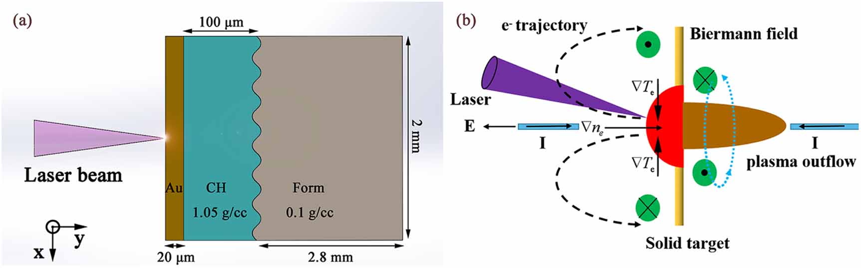
Figure 1(a) illustrates the initial simulation setup, with a total energy of EL = 1000 J, a wavelength of λL = 0.351 μm, and a focal spot radius of RL = 100 μm. A trapezoidal flat-top laser pulse has pulse durations of τL = 0.351 μs and a rising and falling edge of δT = 0.1 ns, incidents along the positive direction of the y-direction. The laser intensity is approximately 1.6 × 10¹⁵ W cm−2. The 2D simulation area is the x–y plane, and the simulation box size is set to Lx × Ly = 2400 μm × 3200 μm with a maximum resolution is 1 μm × 1 μm. Furthermore, the boundary condition of free outflow disturbing the plasma is used in the simulation to avoid the magnetic field being reflected by the boundary and the central region. Figure 1 illustrates the structural characteristics of each target layer, composed of the Au layer followed by the polystyrene (CH) modulation layer and foam layer. The Au layer mass density is estimated as ρAu = 19.32 g cm−3, and Lx × Ly = 2000 × 20 μm2 in area. The mass density of CH is 1.05 g cm−3, the area is Lx × Ly = 2000 × 120 μm2, and the width of the base is 100 μm. The density of the foam layer is 0.1 g cm−3. The initial single-mode sinusoidal disturbance is introduced into the substrate interface between the CH layer and the foam layer, λ0 = 60 μm, with a peak valley amplitude of A0 = 20 μm (y = 20cos(2πx/60). The rest of the whole simulation area is filled with low-density helium (10−6 g cm−3).

Figure 1. (a) The initial simulated setup for generating RTI using a laser-driven modulation target. The purple cone represents the laser pulse. (b) Schematic diagram of the Biermann seed magnetic field in the plasma.
Download figure:
Standard image High-resolution imageWhen an intense nanosecond laser drives the thin solid target, super-hot electrons are formed on the laser radiation surface due to the radiation pressure of laser light. Moreover, super-hot electron flow can be transported into the target. Meanwhile, one plasma bubble is generated on the surface of the target. In addition, the mass of an electron is small and can be quickly accelerated and heated by the laser radiation pressure forming an electronic compression layer. The plasma temperature and pressure rise rapidly, and a large temperature gradient and a pressure gradient are formed in the normal direction of the back surface of the target, causing an isothermal expansion and thermal expansion of plasma along the normal direction of the back surface of the target. Since the plasma near the laser focal spot is hotter, and the temperature along the laser path is also higher, the temperature gradient is parallel to the target surface when viewed perpendicular to the laser path. The expansion direction of the plasma is mainly along the normal direction of the target surface. Therefore, the direction of the plasma density gradient points to the normal direction perpendicular to the target surface. The inhomogeneity of the irradiated area will increase the inconsistency in the directions of the temperature gradient and the density gradient. During the expansion of the plasma flow, the electrodynamic force ( ) is generated by the inconsistency of the temperature gradient and the density gradient, which cause the thermal current and induces the self-generated magnetic field. The self-generated magnetic fields are toroidal and quasi-steady, which are concentrated on a semispherical shell surrounding the ablated plasma bubble. They have maximum amplitude near the edge (
 ). The schematic diagram is shown in figure 1(b). For the target type shown in figure 1(a), when the laser beam is injected from one side of the Au shielding layer, the plasma bubble in front of the target, a forward shock wave, and the plasma outflow behind the target will be generated. The plasma outflow will carry the Biermann seed magnetic field to transmit in the CH. Fluid-type instabilities are caused during the shock wave, continuously accelerating the disturbance interface behind the target. In the FLASH, we can add permanent magnets to generate an external magnetic field before the laser loading. In the 2D x–y plane, an external magnetic field in the x and y directions can be set.
Here, laser-driven interface instability is analogous to the interaction process between SNR and interstellar media. By introducing an external magnetic field, we can simulate the ambient magnetic field in the interstellar medium. The introduction of the external magnetic field may lead to two results: amplifying the environmental magnetic field and suppressing the interface instability by the external magnetic field. The external magnetic field must be weak enough to ensure that the development of the fluid-type instabilities (RTI, RMI) are not suppressed. Sano et al indicate that there is a critical magnetic field that suppresses the RTI and RMI. Only when the strength of the initial applied magnetic field is lower than the critical magnetic field, the interface instability can develop freely. This phenomenon can be characterized by comparing the values of the dimensionless parameter Alfvén number RA ( ) (where u is the average velocity of interface instability and vA is the Alfvén velocity) [23, 35, 36]. When RA< 1, the Lorentz force acting on the fluid will firmly stabilize the interface instability [37–39]. Otherwise, if RA ⩾ 1, the external magnetic field will not inhibit the development of the interface instability. However, it will be compressed and amplified.
The simulation in this study involves six cases, as presented in table 1: Case 1–4 correspond to the single-mode disturbance. Case 1 has no a magnetic field, Case 2 has an applied magnetic field in the x-direction corresponding to 100 G, Case 3 has an external magnetic field in the x-direction corresponding to 1000 G, and Case 4 has an applied magnetic field in the y-direction corresponding to 1000 G. Case 5 and Case 6 corresponding to the flat-target, with the external magnetic field in x-direction corresponding to 1000 G and without a magnetic field, respectively. The Biermann self-generated magnetic field is considered in all cases: its initial applied magnetic field intensity B0 involved is far less than the critical magnetic field intensity Bcri ∼ 3.4 × 10⁵ G.
Table 1. Comparison of the simulation parameters under different initial conditions.
| Cases | Perturbance mode | Perturbation equation (µm) | Applied magnetic field (Gauss) |
|---|---|---|---|
| 1 | Single-mode | y = 20cos(πx/30) | 0 |
| 2 | Single-mode | y = 20cos(πx/30) | x-100 |
| 3 | Single-mode | y = 20cos(πx/30) | x-1000 |
| 4 | Single-mode | y = 20cos(πx/30) | y-1000 |
| 5 | Flat target | No | x-1000 |
| 6 | Flat target | No | 0 |
3. Results and discussion
Figure 2 illustrates the electron density distributions at 8 ns, 16 ns, 24 ns, and 32 ns, respectively, without an external magnetic field. The delay time starts from the time of the laser pulse injection. Initially, the laser beam is injected into the Au shielding layer (injection position: (1000 mm, 0)). Then, the laser passes through the Au shielding layer to ablate the CH and generates a forward shock wave. The shock wave propagates through the CH to the low-density foam, and the shock wave continuously accelerates and disturbs the interface growth process, causing RMI. When the laser pulse ends, the shock wave evolves into a blast wave, which causes the system to decelerate, thereby generating an RTI in the reference frame of the interface [40, 41]. RTI occurs at the fluid interface where the density is not uniformly distributed. When the directions of the pressure gradient and the density gradient are opposite, the interface disturbance grows, and the gradual instability eventually causes to a violent, turbulent mixing phenomenon. When the interface between fluids with different densities is accelerated by the shock wave, the interface fluid mixing phenomenon is called RMI. Here, the evolution process of RTI can be divided into three stages: linear growth, nonlinear growth, and turbulent mixing. In the linear growth stage, fluids of different densities penetrate each other, vorticity deposition occurs, and the initial disturbance on the interface increases exponentially with time, as depicted in figure 2(a). When the perturbation amplitude A reaches the equivalent of the initial perturbation wavelength λ0, it suggests the start of nonlinear growth. During this period, the light fluid enters the heavy fluid to form bubbles, and the heavy fluid enters the lighter fluid to form a mushroom-spike structure. In the later stage, entrainment occurs at the tail of the RTI spike, resulting in secondary instability, namely KHI, as depicted in figure 2(b). We will briefly describe the mixing zone height and interface height of RTI as MZ and H respectively. In the turbulent mixing stage, the disturbed interface deforms violently. The spikes are gradually broken vortices merge and transform into turbulent flow. Figures 2(c) and (d) illustrates evidence of vortex-merging; the more severe turbulent mixing appears later.
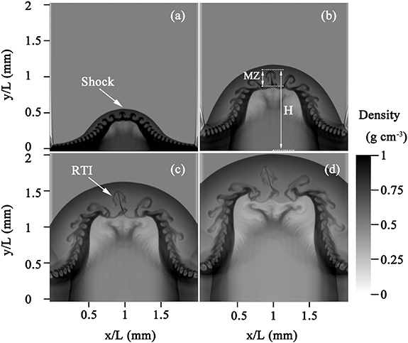
Figure 2. In the absence of an applied magnetic field, the electron density distribution at different times (g cm−3). Figures (a)–(d) correspond to 8 ns, 16 ns, 24 ns, and 32 ns, respectively. The MZ is the height of RTI mixing zoon, and the H is the height of the RTI interface.
Download figure:
Standard image High-resolution imageFigure 3 illustrates a snapshot of density distribution at 30 ns for four cases of different applied magnetic fields under the same initial disturbance mode. Figures 3(a)–(d) correspond to no applied magnetic field, 100 G in the x-direction, 1000 G in the x-direction, and 1000 G in the y-direction, respectively. The results illustrate that RTI in all four cases has entered the stage of nonlinear growth, gradually transforming into the turbulent mixing, the structure of the bubble spike and the shock wave interface of RTI tend to be consistent. This qualitative finding confirms that the introduced external magnetic fields will not affect the dynamics of RTI evolution. At 0–30 ns, the height of the explosion wave interface is 1900 μm, so the average velocity is  63.3 km s−1, and the RTI interface height is H = 1750 μm. The average development speed is
  = 58.3 km s−1. At the time of 30 ns, the instantaneous velocity of the explosive wave interface is us
= 35 km s−1, the instantaneous velocity of the RTI interface is uH
= 30 km s−1, and the mix zone (MZ) height of RTI is 390 μm. The MZ average development speed is um
= 13 km s−1, and the of speed sound is
= 58.3 km s−1. At the time of 30 ns, the instantaneous velocity of the explosive wave interface is us
= 35 km s−1, the instantaneous velocity of the RTI interface is uH
= 30 km s−1, and the mix zone (MZ) height of RTI is 390 μm. The MZ average development speed is um
= 13 km s−1, and the of speed sound is  = 46 km s−1. The results demonstrate that in the linear growth stage, RTI develops at supersonic speed, enters the nonlinear growth and turbulent mixing stage, and gradually decreases to subsonic speed.
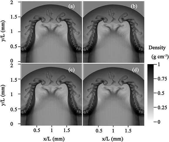
Figure 3. Snapshots of the electron density distribution at the time of 30 ns. Figures (a)–(d) respectively correspond to the case without the external magnetic field, with 100 G applied in the x-direction, with 1000 G applied in the x-direction, with 1000 G applied in the y-direction.
Download figure:
Standard image High-resolution imageThe magnification effect of the magnetic field is examined. With Case 3 as an example, the magnetic field intensity distributions in the x–y plane at 8 ns, 16 ns, 24 ns, and 30 ns are depicted in figure 4, respectively. The results reveal that the substantial magnetic field area is distributed near the top of the mushroom-shaped spike. During the entire evolution of RTI, there is an apparent mutual extrusion with the applied magnetic field in the x-direction, so that the kinetic energy of the plasma flow near the interface of the RTI spike is partially converted into magnetic field energy. Consequently, a more significant magnetic energy gradient exists at the spike interface.
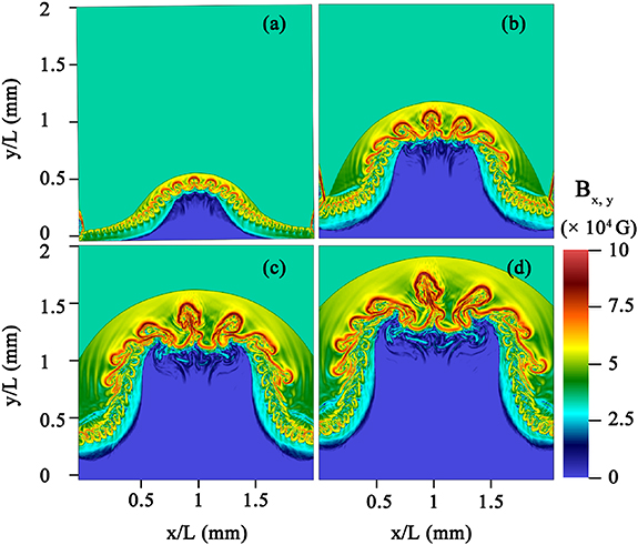
Figure 4. Snapshots of the distribution of the external magnetic field near the RTI evolution area at different time points. Figures (a)–(d) correspond to 8 ns, 16 ns, 24 ns, and 30 ns respectively.
Download figure:
Standard image High-resolution imageAs depicted in figure 4(d), at 30 ns, the maximum value of the magnetic field strength in the RTI evolution region is approximately 9 × 10⁴ G, which is magnified by ∼90-fold. The ratio of magnetic energy to kinetic energy is:

 ≈ 0.75. The magnetic diffusion time
  = 30.6 ns (H= 1.75 mm is the RTI interface height, and η is the magnetic diffusivity) indicates that the magnetic field has penetrated the plasma region at this time, and the plasma near the RTI evolution region is fully magnetized. Furthermore, the plasma β value is approximately 2 × 10⁴ (
 ), and the Alfvén velocity is vA= 1.27 km s−1 (
 ), the corresponding Alfvén number is RA ≈ 23.6 (
 ). This indicates that the plasma is dominated by thermal pressure. However, the amplified magnetic field does not alter the dynamics of RTI evolution. Based on the ideal MHD theory, with Case 3 as an example, the linear growth rate of RTI when considering the magnetic field is [41, 42],

where Atwood number  = 0.81, ρ1 corresponds to the initial density value of the CH modulation layer, ρ2 corresponds to the low-density foam initial density of the material. The equivalent gravitational acceleration
  = 4.5 × 10¹¹ m s−2, wave vector
  = 1.05 × 10⁴ m−1, the magnetic field strength B = 9 × 10⁴ G,
  ns is derived, which is consistent with the simulation results. After 16.1 ns, RTI enters a nonlinear growth stage, as shown in figure 2(b).
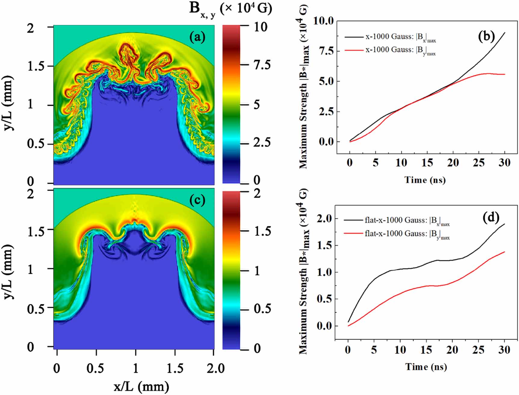
Figure 5 illustrates the change in the maximum magnetic field strength |B|max with time in Case 3 and 5, which explains the amplification mechanism of the external environmental magnetic field. Figures 5(a) and (c) correspond to the magnetic field strength distribution in the x–y plane at 30 ns, respectively. Figures 5(b) and (d) correspond to the change curve of |Bx |max with time. The solid black line represents the maximum modulus |Bx |max of the magnetic field strength component in the x-direction, and the solid red line represents the maximum modulus |By |max of the magnetic field strength component in the y-direction. Figure 5(a) shows that the substantial magnetic field area is distributed near the top of the mushroom spike. Combined with the previous analysis, figure 5(b) shows that during 0–30 ns, RMI, RTI, KHI, and other fluid instabilities are coupled, gradually transforming to turbulence, and the magnetic field in the x-direction is constantly stretched, twisted, and amplified. At the moment of 30 ns, |Bx |max= 9.0 × 10⁴ G. In contrast, the magnetic field component in the y-direction increases linearly during the period of 0–20 ns and gradually saturates after 20 ns, |By |max= 4.9 × 10⁴ G. Figures 5(c) and (d) correspond to the flat target. No apparent interface instability exists in the flat target driven by an intense laser. The magnetic field components in the x and y-direction also gradually increase with time. At this time, the magnetic field amplification may be caused by the compression effect of the external environmental magnetic field of the plasma outflow, the non-uniformity of the laser focal spot, and the numerical noise of the simulated grid size. At 30 ns, |Bx |max= 1.9 × 10⁴ G, |By |max= 1.38 × 10⁴ G. By comparing figures 5(b) and (d) confirm that amplifying the external environmental magnetic field is caused primarily by fluid instability.

Figure 5. Time evolution of the magnetic field. (a) and (c) Snapshots of the distribution of the external magnetic field in Case 3 and Case 5 at 30 ns. (b) and (d) Time evolutions of the maximum strength of the magnetic field for each component |Bx |max.
Download figure:
Standard image High-resolution imageNon-parallel gradients of the electron density and temperature in a laser-heated plasma generate a self-generated magnetic field through the Biermann battery mechanism ( , where Pe
is electron pressure, ne
is electron density) [43, 44]. In the 2D x–y plane, the Biermann magnetic field is expressed as a toroidal component BZ
perpendicular to the paper surface. However, it has no contribution to the x–y plane. Figures 6 and 7 show the distribution of Biermann magnetic field intensity for a single-mode modulation target and a flat target without an external magnetic field, respectively. The data for 8, 16, 24, and 30 ns are depicted. Figure 6 shows that during the evolution of RTI, the Biermann magnetic field around the RTI spike is alternately positive and negative and gradually attenuates in time with the diffusion of plasma outflow. At 30 ns, the maximum strength of the Biermann magnetic field decreases to 2 × 10⁴ G. Comparing figures 6 and 7 indicate that, for a flat target, the temperature gradient and density gradient behind the target decrease because of the absence of an initial disturbance. At 30 ns, the maximum strength of the Biermann magnetic field is only 1.7 × 10⁴ G. The results show that RTI can amplify Biermann magnetic field
, where Pe
is electron pressure, ne
is electron density) [43, 44]. In the 2D x–y plane, the Biermann magnetic field is expressed as a toroidal component BZ
perpendicular to the paper surface. However, it has no contribution to the x–y plane. Figures 6 and 7 show the distribution of Biermann magnetic field intensity for a single-mode modulation target and a flat target without an external magnetic field, respectively. The data for 8, 16, 24, and 30 ns are depicted. Figure 6 shows that during the evolution of RTI, the Biermann magnetic field around the RTI spike is alternately positive and negative and gradually attenuates in time with the diffusion of plasma outflow. At 30 ns, the maximum strength of the Biermann magnetic field decreases to 2 × 10⁴ G. Comparing figures 6 and 7 indicate that, for a flat target, the temperature gradient and density gradient behind the target decrease because of the absence of an initial disturbance. At 30 ns, the maximum strength of the Biermann magnetic field is only 1.7 × 10⁴ G. The results show that RTI can amplify Biermann magnetic field  ).
).
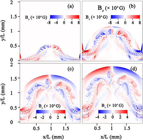
Figure 6. Spatial distribution of Biermann magnetic field intensity in RTI evolution region in the case of single-mode modulation target without external magnetic field. Figures (a)–(d) correspond to 8 ns, 16 ns, 24 ns and 30 ns respectively in the unit of G.
Download figure:
Standard image High-resolution image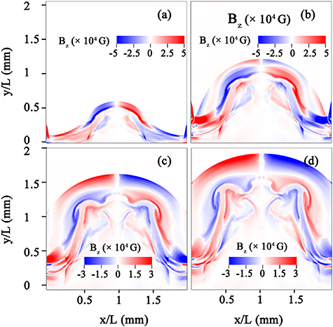
Figure 7. Spatial distribution of Biermann self-generated magnetic field intensity in the case of flat target without external magnetic field. Figures (a)–(d) correspond to 8 ns, 16 ns, 24 ns and 30 ns respectively in the unit of G.
Download figure:
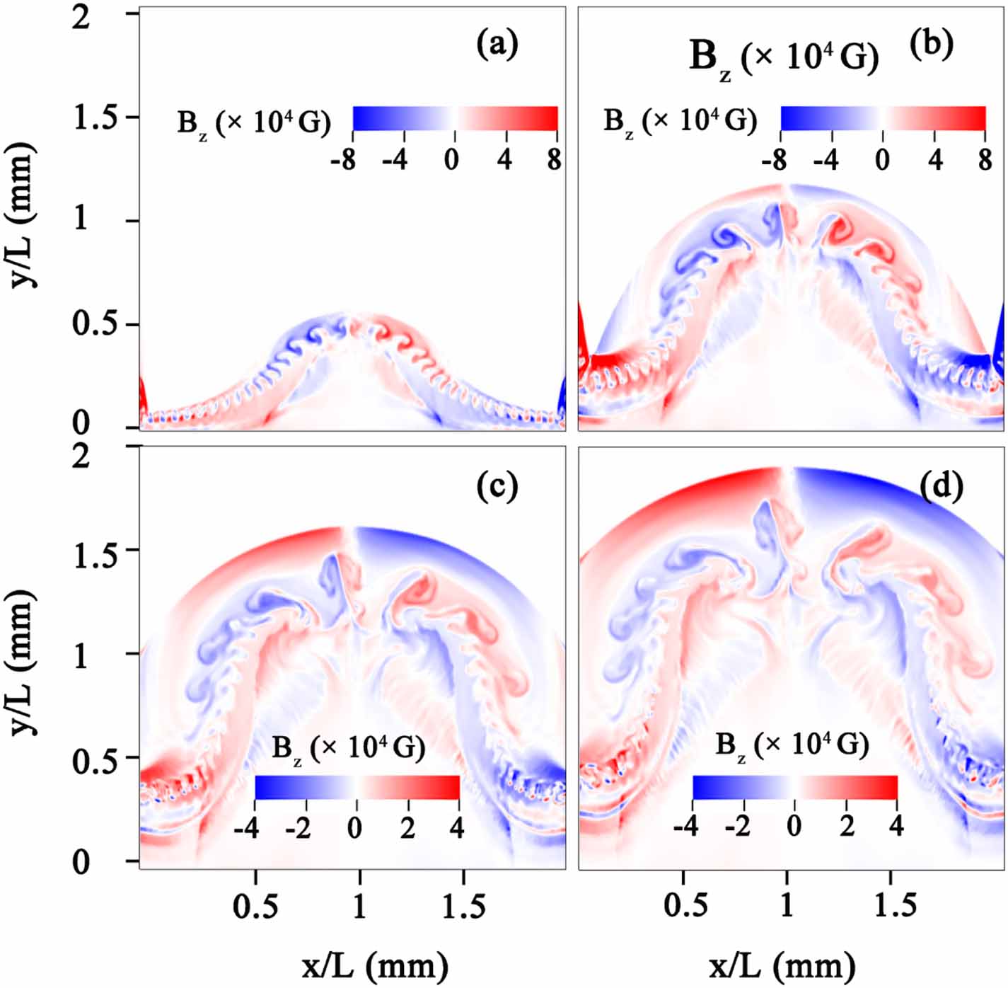
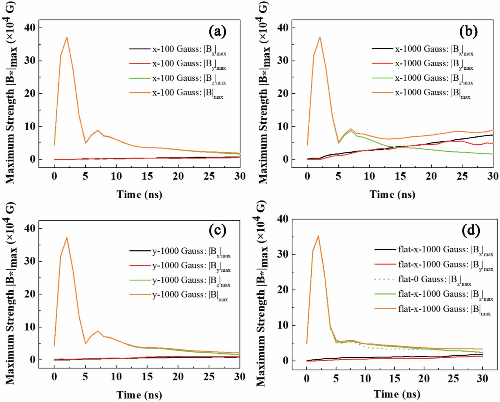
Standard image High-resolution imageThe contribution of external environmental magnetic fields and the Biermann magnetic field during the magnetic field amplification are compared further. Figure 8 systematically illustrates the change in modulus |B*|max of the maximum magnetic field in each direction with time under different initial conditions. Figures 8(a)–(c) illustrate the single-mode perturbation, corresponding to the case of applying a 100 G magnetic field in the x-direction, a 1000 G magnetic field in the x-direction, and a 1000 G magnetic field in the y-direction, respectively. Figure 8(d) shows the case of the flat target. In figure 8, the solid black line, red, green, and orange lines represent the X direction, the y-direction, the z-direction, and the total maximum modulus |B|max ( ), respectively. Figure 8 illustrates that the Biermann magnetic field intensity increases rapidly with laser injection, reaching a maximum value |Bz
|max= 3.8 × 10⁵ G at 2 ns. When the laser pulse ends, the Biermann magnetic field intensity decreases rapidly.
), respectively. Figure 8 illustrates that the Biermann magnetic field intensity increases rapidly with laser injection, reaching a maximum value |Bz
|max= 3.8 × 10⁵ G at 2 ns. When the laser pulse ends, the Biermann magnetic field intensity decreases rapidly.
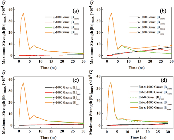
Figure 8. Time evolutions of the maximum strength of the magnetic field for each component in (a)–(c) the modulated-target case and (d) the flat-target case. The laser irradiation is from t = 0–2 ns. The amplified magnetic fields |Bx
|max, |By
|max, and |Bz
|max is depicted by the black, red and green solid line respectively. The orange solid line indicates the total magnetic field ( ). Figures (a)–(c) correspond to the initial application of a 100 G in the x-direction, the initial application of a 1000 G in the x-direction, and the initial application of a 1000 G in the y-direction. (d) Corresponding to the case of a flat-target, the solid line represents the initial applied 1000 G in the x-direction, and the green dotted line represents the case of no external magnetic field, that is, the Biermann magnetic field.
Download figure:
Standard image High-resolution imageIn figure 8(a), at 30 ns, |Bz |max= 2 × 10⁴ G. Comparing figures 8(a) and (b), it can be found that when 100 G external magnetic field is applied in the x-direction, Bx is compressed and amplified 76 times at 30 ns, reaching 7.6 × 10³ G, during the evolution of RMI, KHI, and RTI, the magnetic field at the interface is continuously compressed and deformed, and the magnetic field component in the y-direction is generated at the same time. At this time |By |max= 6.2 × 10³ G, lower than Biermann magnetic field (∼2.0 × 10⁴ G). When the external magnetic field of 1000 G in the x-direction is applied, Bx and By increase linearly with time. At 30 ns, |Bx |max= 9.0 × 10⁴ G, |By |max= 4.9 × 10⁴ G, which exceeded the strength of the Biermann magnetic field. Comparing figures 8(b) and (c), the results show that the applied magnetic field is not significantly amplified after the introduction of the external magnetic field in the y-direction. At 30 ns, |Bx |max= 9.0 × 10³ G, |By |max= 1.0 × 10⁴ G, which indicates that the external magnetic field in the x-direction is dominant in the turbulent magnetic field amplification phenomenon, which is induced by interface instability. Figures 8(b) and (d) illustrates that under the condition of the flat target when 1000 G external magnetic field is introduced in the x-direction, at the time of 30 ns, |Bx |max= 1.9 × 10⁴ G, |By |max= 1.4 × 10⁴ G. Consequently, adding 1000 G in the x-direction compresses and amplifies the magnetic field by introducing the initial disturbance. For a flat target, the external magnetic field will be amplified 19 times because of the inhomogeneity of the laser focal spot or the numerical noise of the simulated grid size scale. The amplified magnetic field is much weaker than that for instability. Figure 8(d) reveals that the dotted and solid green lines almost coincide, indicating that the external environmental magnetic field does not contribute to the Biermann magnetic field.
Figure 9 shows the discrete Fourier spectrum of the magnetic energy density M(ω) as a function of frequency ( , the unit is G2). M(ω) is the average magnetic field energy density of the entire RTI evolution region. The ordinate of the figure is
  , and the abscissa is lg(ω). In figure 9, the red, green, and orange dotted lines correspond to the initial applied magnetic field of 100 G and 1000 G along the x-direction, and 1000 G in the y-direction, where the single-mode disturbances are introduced in all three cases. The purple dotted line in figure 9 corresponds to the flat target in which the initial external magnetic field is 1000 G in the x-direction. Figures 9(a) and (b) are the magnetic energy spectrum in x- and y-directions. Consistent with Schekochihins [45] and Ruzmaikin [46], under the condition of Rm
∼ 1, on the spatial scale, the magnetic energy is:
, and the abscissa is lg(ω). In figure 9, the red, green, and orange dotted lines correspond to the initial applied magnetic field of 100 G and 1000 G along the x-direction, and 1000 G in the y-direction, where the single-mode disturbances are introduced in all three cases. The purple dotted line in figure 9 corresponds to the flat target in which the initial external magnetic field is 1000 G in the x-direction. Figures 9(a) and (b) are the magnetic energy spectrum in x- and y-directions. Consistent with Schekochihins [45] and Ruzmaikin [46], under the condition of Rm
∼ 1, on the spatial scale, the magnetic energy is:

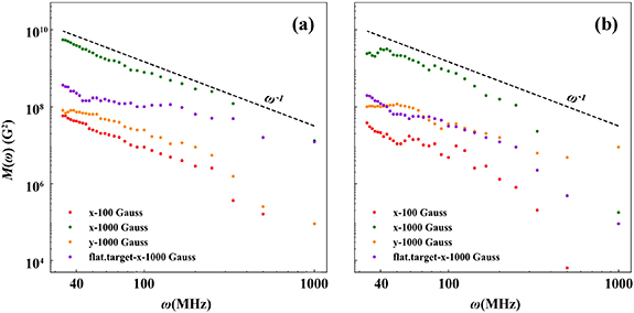
Figure 9. Frequency spectrum of the magnetic field. Plot of simulated magnetic energy spectrum  , where B(ω) is the average magnetic field in total RTI evolution region. Figures (a) and (b) represent the frequency spectrum of the magnetic field components in the x and y directions under different initial conditions, respectively. The red dotted line corresponds to the initial applied magnetic field of 100 G in the x-direction, single-mode disturbance, the green dotted line corresponds to the initial applied magnetic field of 1000 G in the x-direction, single-mode disturbance, and the orange dotted line corresponds to the initial applied magnetic field of 1000 G in the y-direction, single-mode disturbance, the purple dotted line corresponds to the initial applied magnetic field of 1000 G in the x-direction, and the flat-target.
Download figure:
Standard image High-resolution imageIf the kinetic energy density E(k) ( ) conforms to the Kolmogorov turbulence spectrum,
  , then the magnetic energy density
  . When Rm
≫ 1, the magnetic energy density M(k) ∼ B0
2
k−1, and the magnetic energy density, and the turbulent kinetic energy are evenly divided. Here, the spectral indices of the magnetic energy index M(ω) obtained from the four cases in figure 9 are close to ω−1. For the initial addition of 1000 G and single-mode disturbance in the x-direction, the Reynolds number
. When Rm
≫ 1, the magnetic energy density M(k) ∼ B0
2
k−1, and the magnetic energy density, and the turbulent kinetic energy are evenly divided. Here, the spectral indices of the magnetic energy index M(ω) obtained from the four cases in figure 9 are close to ω−1. For the initial addition of 1000 G and single-mode disturbance in the x-direction, the Reynolds number  2 × 10⁸, the magnetic Reynolds number
  100, and the magnetic Prandtl number
  = 5 × 10⁻⁷, the M(k) ∼ k−1 condition is satisfied in this case. If a constant speed of the plasma flow is assumed,
  , the frequency information can substitute the spatial fluctuation of the magnetic field. When the plasma velocity is uH
= 30 km s−1 and the frequency is 30 MHz, the unstable turbulence scale is close to 1000 μm, which is much larger than the initial disturbance (∼20 μm). Furthermore, after comparing the distribution of the green and the orange dotted lines in figures 9(a) and (b), the green dotted line is two orders of magnitude higher on average than the orange dotted line, indicating that the applied magnetic field mainly dominates the magnification effect of the turbulent magnetic field in the x-direction. This finding also be corroborated by the comparison in figures 8(b) and (c).
, the frequency information can substitute the spatial fluctuation of the magnetic field. When the plasma velocity is uH
= 30 km s−1 and the frequency is 30 MHz, the unstable turbulence scale is close to 1000 μm, which is much larger than the initial disturbance (∼20 μm). Furthermore, after comparing the distribution of the green and the orange dotted lines in figures 9(a) and (b), the green dotted line is two orders of magnitude higher on average than the orange dotted line, indicating that the applied magnetic field mainly dominates the magnification effect of the turbulent magnetic field in the x-direction. This finding also be corroborated by the comparison in figures 8(b) and (c).
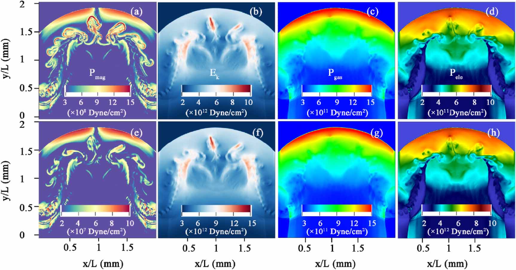
Figure 10 shows the distributions of magnetic field energy density, kinetic energy density, background gas pressure, and electron thermal pressure, respectively. All subgraphs of the figure 10 correspond to 30 ns. Different rows represent different simulation cases, and different columns represent different physical information. The first row corresponds to a single mode, in which 1000 G is initially applied in the x-direction, and the second row corresponds to a single mode in which no external magnetic field is applied. Figure 10 shows that the spatial distribution of the background gas pressure and the electron thermal pressure is almost the same in both cases, indicating that the introduction of the external magnetic field in the x-direction will not significantly impact the background gas pressure and the electron thermal pressure. In contrast, with the 1000 G magnetic field in the x-direction, the kinetic energy density decreases, the maximum |Ek |max changes from 1.5 × 10¹³ dyn cm−2 to 1.0 × 10¹³ dyn cm−2, and the magnetic field energy density increases, the maximum |Pmag |max is about 1.5 × 10⁹ dyn cm−2. However, the evolution of fluid instability is still dominated by kinetic energy density and thermal pressure. The results show that RTI in all two cases has entered the stage of nonlinear growth, gradually transiting to the turbulent mixing process. Similar conclusions can be drawn from the distribution of the vorticity field in figure 2 above.
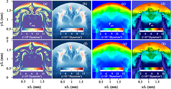
Figure 10. The distributions of magnetic field energy density, kinetic energy density, background gas pressure, and electron thermal pressure, respectively. Different rows represent different simulation cases, and different columns represent different physical information. The two rows represent Case 3 and Case 1, respectively, and all subgraphs correspond to 30 ns.
Download figure:
Standard image High-resolution imageHere, it needs to be clear that we do not simulate the case of collisionless plasma. When there is a magnetic field, the magnetic field will constrain particles. The presence of a magnetic field reduces sharply the particle mean free path, in place of the Coulomb mean free path, we should use the Larmor radius ( ) to analyze [47]. In this work, the Lamar radius of electrons and ions are rLe = meu/eB ∼ 2.13 × 10⁻²
μm, rLI = miu/ZeB ∼ 0.01 mm, respectively. The system size is L = 2 mm, the ratio of the electron Larmor radius to the system size, rLe/L is approximately 1.06 × 10⁻⁵, and the ratio of the ions Larmor radius to the system size rLi/L is approximately 5 × 10⁻³. This shows that the radius of gyration is far smaller than the system scale due to the enhancement of magnetic field strength, so this is essentially equivalent to the collision process. Therefore, we can use the MHD method to study the magnetic field amplification induced by turbulence in SNRs.
) to analyze [47]. In this work, the Lamar radius of electrons and ions are rLe = meu/eB ∼ 2.13 × 10⁻²
μm, rLI = miu/ZeB ∼ 0.01 mm, respectively. The system size is L = 2 mm, the ratio of the electron Larmor radius to the system size, rLe/L is approximately 1.06 × 10⁻⁵, and the ratio of the ions Larmor radius to the system size rLi/L is approximately 5 × 10⁻³. This shows that the radius of gyration is far smaller than the system scale due to the enhancement of magnetic field strength, so this is essentially equivalent to the collision process. Therefore, we can use the MHD method to study the magnetic field amplification induced by turbulence in SNRs.
Next, we compare the turbulent magnetic field amplification caused by interface instability simulated in the laboratory with the local turbulent magnetic field amplification in the SNR shell in astrophysics. According to the similarity principle [17, 18, 48], the correlation between the two systems can be described by several important dimensionless parameters, such as Reynolds number  2 × 10⁸≫1, Peclet number PeL = Lv/κ ∼ 60 > 1, magnetic Reynolds number
  ∼ 100 > 1, where ν is the dynamic viscosity, κ is the thermal diffusivity. These dimensionless parameters of laboratory plasma and typical SNR parameters are listed in table 2. The two systems should meet the following scaling law: rSNR = arlab, ρSNR = bρlab, PSNR = cPlab,
  ,
,  ,
,  , where the subscripts 'lab' and 'SNR' represent laboratory simulation system and SNR system, respectively. Here we mainly compare with Tycho's SNR (SN 1572) outer shell plasma environment, the parameters are shown in table 2 [23, 48–52]. Table 2 also lists the relevant physical parameters of typical SNR in detail, such as the length is 1 pc (1 pc ≈ 3.1 × 1018cm), the typical time scale is 300 years. The typical physical parameters of the initial addition of 1000 G in the x-direction and single-mode disturbance are also listed. By comparing the free transformation parameters of the two systems, we can conclude that our simulations can be amplified into the SNR shell scale a = 1019, b = 10−24, c = 10−20. The two systems are very similar well. The laboratory plasma can be used to explore the phenomenon of local magnetic field enhancement in SNR, which will help further the understanding of the evolution of interstellar magnetic fields.
Table 2. Comparison of the SNR with the laboratory plasma under the scaling laws.
| Parameters | Simulated laser-produced plasma | SNR | Scaled to SNR | |
|---|---|---|---|---|
| Material | CH | H | ||
| Thermal pressure | P | 5 × 10¹¹ Pa | 5 × 10⁻⁹ Pa | 5 × 10⁻⁹ Pa |
| Mass density | ρ | 0.5 g cm−3 | 2 × 10⁻²⁴ g cm−3 | 5 × 10⁻²³ g cm−3 |
| Electron number density | ne | 3 × 1022 cm−3 | 1 cm−3 | 0.03 cm−3 |
| Time | t | 30 ns | 300 years | 95.24 years |
| Temperature | T | 13.8 eV | 30 keV | — |
| Plasma velocity | u | 30 km s−1 | 3 × 10³ km s−1 | 3 × 10³ km s−1 |
| System length | L | 2 mm | 1 pc | 0.65 pc |
| Kinematic viscosity | ν | 3 × 10⁻¹¹cm2 s−1 | 3 × 1013cm2 s−1 | — |
| Reynolds number |

| 2 × 10⁸ | 2 × 10⁷ | — |
| Magnetic diffusivity | η | 6 × 103cm2 s−1 | 2 cm2 s−1 | — |
| Magnetic Reynolds number |

| 100 | 3 × 1024 | — |
| Magnetic Prandtl number |

| 5 × 10⁻⁷ | 2 × 10¹⁷ | — |
| Magnetic field | B | 8 × 10⁴ G | 10−5 G | 8 × 10⁻⁶ G |
| Magnetic pressure | PB | 2.5 × 10⁷ Pa | 4 × 10⁻¹³ Pa | — |
| Plasma β |
| 2 × 10⁴ | 104 | — |
| Alfvén speed |
| 1.27 km s−1 | 20 km s−1 | — |
| Alfvén number |

| 23.6 | 15 | — |
The amplified magnetic field in SNR plays an essential role in many physical processes. Such as in core-collapse supernovae, the role of high magnetic fields in the accretion disk has been suggested to be necessary for the explosion mechanism [53]. Hristov et al studied the influence of magnetic field strength and morphology in Type Ia supernovae and their late-time light curves and spectra. The results suggest that the topology of the magnetic field is set by the burning, independent of the initial strength. In thermonuclear explosions, late-time light curves and spectra (300 days) put the lower limits are found to be 106 G based on the lack of positron transport effect in the expanding envelope [54]. In addition, the presence of a milligauss magnetic field has a critical meaning in the long-standing paradigm of cosmic-ray proton acceleration in young SNRs [55, 56]. Some MHD simulations suggest that turbulent magnetic fields driven by hydrodynamic instabilities may have radially biased velocity dispersions, leading to selective amplification of the radial component and further cosmic-ray production [57, 58]. The remnant of SN 1987A has been proved to be a unique laboratory for investigating particle acceleration in young SNRs [59]. The researchers applied the Fermi acceleration mechanism to the interaction process between the particles near the shock surface and the turbulent magnetic field frozen in the background plasma and gradually developed the 'diffusion shock acceleration' model [60, 61]. This model is widely used to explain the non-thermal distribution of particles (the energy E ∼ PeV) in many high-energy celestial bodies. Moreover, Muller et al [62] studied the impact of a small-scale dynamo in core-collapse supernovae using a 3D neutrino MHD simulation. The results suggest that magnetic fields may be beneficial in neutrino-driven supernovae even without rapid progenitor rotation.
4. Conclusion
This study conducts a 2D numerical simulation of the amplification effect of the turbulent magnetic field in SNRs by an intense laser using FLASH code. The qualitative and quantitative aspects of the physical mechanism of turbulent magnetic field amplification are examined. We investigate and compare the evolution of unstable turbulence under different initial disturbance modes, target types, directions, and intensities of external magnetic fields. We distinguish between the contribution of the Biermann magnetic field and environmental magnetic field during magnetic field amplification and calculate the magnetic energy spectrum and magnetic field amplification ratio. Our findings are summarized as follows:
- (1)The shock wave generated by the laser-driven target accelerates continuously and causes RMI during the growth of the disturbed interface. When the laser pulse ends, the shock wave evolves into an explosion wave, causing the system to decelerate, resulting in RTI in the interface system. There is a secondary instability KHI at the tail of the RTI spike. The turbulent interface system involves several instabilities and complex interactions.
- (2)The fluid motion associated with RTI will stretch the environmental magnetic field, and the intensity is amplified by approximately two orders of magnitude, while the self-generated magnetic field of the Biermann battery process is not significantly amplified (
 ∼ 1.18).
 - (3)The x-direction component of the ambient magnetic field is dominant role in magnetic field amplification. For the case of the external magnetic field of 1000 G in the x-direction and single-mode disturbance, at 30 ns, |Bx |max = 9 × 10⁴ G, |By |max = 4.9 × 10⁴ G, confirming that the maximum strength of the amplified components exceeds the Biermann magnetic field sufficiently (∼1.7 × 10⁴ G).
- (4)Based on the scaling law, the simulation results in this study can be amplified into the SNR shell environment scale. The two systems are similar, which is necessary for explaining the physical mechanism of magnetic field amplification in SNR. The results contribute toward understanding interstellar turbulence and magnetic field evolution. Furthermore, the research results establish a reference for laser-driven magnetized plasma experiments in a robust magnetic environment.

We will conduct relevant experiments in future research. Concerning the target structure in this study, we use the proton radiography and B-dot probe array to obtain the energy spectrum of magnetic field evolution. We expect to clarify the magnification of the magnetic field from experiments and distinguish the contribution of the environmental magnetic field and Biermann magnetic field in amplifying the turbulent magnetic field. This will provide more laboratory evidence support for the amplification effect of the turbulent magnetic field in astronomy and promote laboratory astrophysics development.
Acknowledgments
We thank anonymous reviewers for their valuable comments that well-improved the manuscript. This work was supported by the National Natural Science Foundation of China (Grant Nos. 12205382, 12005305, U2267204, and U2241281), Young Talents Cultivation Fund of China Institute of Atomic Energy (Grant No. YC222412000901), the Strategic Priority Research Program of the Chinese Academy of Sciences (Grant No. XDA25030700), and Key Programs of the Chinese Academy of Sciences (Grant No. QYZDJ-SSW-SLH050). The simulations were carried out on the Beijing super cloud computing center in Beijing. The authors were particularly grateful to Flash Center for Computational Science at the University of Chicago for allowing us to use the FLASH code. Finally, we thank Philip Pape, PhD, from Liwen Bianji (Edanz) (www.liwenbianji.cn) for rounding off the English text of a draft of this manuscript.
Data availability statement
The data cannot be made publicly available upon publication because no suitable repository exists for hosting data in this field of study. The data that support the findings of this study are available upon reasonable request from the authors.