
Abstract
DNA Nanotechnology is being applied to multiple research fields. The functionality of DNA nanostructures is significantly enhanced by decorating them with nanoscale moieties including: proteins, metallic nanoparticles, quantum dots, and chromophores. Decoration is a complex process and developing protocols for reliable attachment routinely requires extensive trial and error. Additionally, the granular nature of scientific communication makes it difficult to discern general principles in DNA nanostructure decoration. This tutorial is a guidebook designed to minimize experimental bottlenecks and avoid dead-ends for those wishing to decorate DNA nanostructures. We supplement the reference material on available technical tools and procedures with a conceptual framework required to make efficient and effective decisions in the lab. Together these resources should aid both the novice and the expert to develop and execute a rapid, reliable decoration protocols.
Export citation and abstract BibTeX RIS

Original content from this work may be used under the terms of the Creative Commons Attribution 4.0 licence. Any further distribution of this work must maintain attribution to the author(s) and the title of the work, journal citation and DOI.
Glossary
| DNA nanostructure | A two-dimensional (2D) or three-dimensional (3D) structure fabricated from DNA using sequence recognition and assembly. This includes tiles, origami, bricks, etc. |
| Decoration | Placement of a functional element onto a DNA nanostructure at a specific location |
| Functional element | A nanoscale object that performs a physical, chemical, biological, and/or informational function, e.g. a protein, peptide, metal nanoparticle, quantum dot, chromophore etc. |
| Addressability | The ability to site-specifically decorate DNA labeled elements at locations on a nanostructure |
| Process steps | Separate actions, or unit processes, that are ultimately used in combination to complete the fabrication of a structure |
| Decoration phases | Categories of process steps including design, assembly, purification, and verification |
| Decoration workflow | A complete set of process steps designed to create the desired product |
| Decoration precision | The standard deviation about the mean functional element position relative to the DNA nanostructure |
| Decoration accuracy | The agreement between a designed inter-element distance and the measured mean separation |
| DNA origami | A structure self-assembled from viral-derived scaffolds (approximately 7000–8000 nt) and synthetic 'staple' strands (30–60 nt) |
| DNA oligomer | Single-stranded DNA (ssDNA) with a short, defined, sequence typically shorter than 1000 nt |
| Domain | A defined sequence of nucleotides that comprises part, or all, of a DNA strand |
| Sticky end | Unpaired single-stranded DNA (ssDNA) connected to either a functional element or nanostructure, intended for later addressability, often a single domain on a larger strand |
| Linker modification | Chemical moiety on a DNA oligomer that will bind to a functional element and/or another chemical modification |
| Spacer sequence | DNA nucleotides between the linker moiety and functional element or DNA nanostructure included to increase the distance, or flexibility, of the connection between them |
| Structural yield | Fraction of successfully assembled nanostructure relative to the reagent DNA or relative to the population of characterized products. For origami, the reagent DNA can be either the scaffold or staple strands |
| Migratory yield | Structural yield evaluated as the fraction of product with the expected mobility |
| Imaging yield | Structural yield evaluated as the fraction of product visibly recognizable as being of the 'correct' shape |
| Oligomer inclusion yield | Structural yield evaluated as the fraction of oligomers included in the structure, or included at the expected position within it |
| Site-Occupancy yield | Fraction of sites on a structure which successfully bind a functional element |
| Functional yield | Fraction of structures which perform the desired function |
| Practitioner | Individual who performs the process steps and conducts the project |
| Note | Notes will highlight considerations or pitfalls |
1. DNA nanostructure decoration
This tutorial assumes that the reader is familiar with the basics of DNA nanofabrication [1] and has read our previous tutorial on DNA origami design [2], or other introductory documents [3–5]. While this guide may be applied to the decoration of any DNA nanostructure, we focus on DNA origami due to its ubiquity.
The DNA nanofabrication toolkit provides many options for decorating nucleic acid nanostructures with functional elements at precise, predetermined locations. This is arguably the most important capability it brings to bottom up self-assembly for two reasons: First, DNA bioconjugation methods are sufficiently mature for even novices to readily label a wide variety of functional nanoparticles, proteins, and macromolecules with DNA. Second, since the sequence of the DNA label can be defined, the labeled object may be targeted to bind to any complementary sequence location on a DNA nanostructure, dramatically enhancing the functionality of the 2D and 3D superstructure. A practitioner may decorate a DNA nanostructure with virtually any nanoscale element at almost any spacing or orientation. This flexibility and control are especially valuable for applications where precise spacing is crucial such as interfacing with biochemical systems [6], controlling plasmonic interactions [7, 8], or complex sensing triggered by multiple conformational changes [9, 10].
We approach the topic of DNA decoration holistically, beginning in section 1 with broad definitions of decoration and an explanation of our rationale for dividing the decoration process into phases. In section 2 we articulate the importance of a holistic approach, i.e. systems engineering. Finally, we elucidate specific techniques for each decoration phase in sections 3 through 6.
Note: This document is meant to serve as a tutorial and as a reference material. By intent, it covers nuances left uncovered in research reports and reviews, but communicates neither the novelty of the former, nor the in-depth attribution of accomplishments of the latter.
As for any reference, different details and nuances will be useful to different practitioners. We encourage those readers with specific questions or interests to navigate directly to the relevant section.
Section 1: decoration and its applications
Section 2: the importance of systems engineering to decoration
Section 3: the design of decoration including addressing, accuracy, and precision
Section 4: decorated nanostructure formation, from basic thermodynamics to common protocols
Section 5: purification of decorated nanostructures and challenges thereof
Section 6: verification of decorated nanostructures and uncertainty thereof
1.1. An example decoration workflow
As this tutorial's scope encompasses the breadth of conceptual tools and experimental techniques required to plan a DNA nanostructure decoration workflow it is infeasible to provide protocols for all, or even a portion of the techniques we discuss.
However, it is worth briefly describing how a decoration workflow might proceed in lab to provide a sense of the time investment required and to explain why we advocate for a holistic approach in planning.
Figure 1 illustrates the steps required for the following counter-factual example (example inspired by [11]). Assume the existence of some redox active enzyme that can be labeled with DNA without impairing function. Semiconducting particles with appropriate band gaps can, when in proximity to the enzymes, optically pump them to provide energy. To create the enzyme's product from its substrate and light, one might desire a surface with densely packed, but regularly spaced enzyme-nanoparticle clusters, over which one could flow the enzyme's substrate during exposure to light.
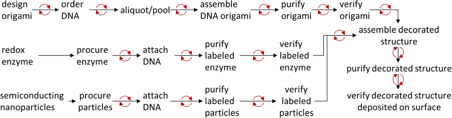
Figure 1. Example workflow, where red circular arrows indicate steps at which iterative troubleshooting may be necessary.
Download figure:
Standard image High-resolution imageDesigning of an origami that can cluster the enzyme and nanoparticles, choosing the labeling chemistries, and making plans for purification and verification will typically take from a month to a few months. Procuring the DNA, enzymes and nanoparticles often take slightly less than a month.
The DNA strands are pooled together into aliquots to accommodate variations of a structure with different decoration spacings or locations by grouping the strands based on which shared structure variants they will create. This usually takes a few days.
After this step a decoration project is a hierarchy of assembly steps, purification steps, and verification steps, each taking between a few hours and a few days. For example, to assemble origami one would mix buffer, salt, viral scaffold strand, structural staple pools, and the modified strands which address the decoration, and perform an overnight thermal anneal. The product origami would be purified from the reagents, e.g. by filter centrifugation, and the assembly would be verified, e.g. by atomic force microscopy. Analogous steps would be performed to label the enzymes and nanoparticles.
The labeled nanoparticles, enzymes, and origami would then be combined, annealed, purified, and deposited on a surface for verification and performance testing.
If every step works as intended, this could take as little as two to three months in total. Unfortunately, troubleshooting is unavoidable, and one only rarely knows why steps fail.
To isolate a failure mode, one works iteratively backwards from the failure point. For example, if a decorated structure fails to assemble one might confirm that the particles or enzymes really are labeled with the correct strand. It is not unusual to work as far back as re-pooling DNA strands or re-evaluating an entire nanostructure design.
Troubleshooting time can have a factorial dependence on project complexity and represents the bulk of the costs for any decoration project. Optimizing troubleshooting through careful holistic planning is crucial.
1.2. Decoration process
Given the broad range of possibilities (type of nanofabrication, functional element type, spacing, etc), there is considerable variation in decoration workflows. We divide these workflows into phases and the phases into process steps. Process steps include designing a DNA nanostructure, fabricating it, purifying it from its constituent oligomers, etc. The number of steps increases with each additional functional element.
We define phases of related steps as: design, assembly, purification, and verification. In design, the nanostructure is drafted and the functional elements, linker chemistries, and sticky end DNA sequences are chosen. In assembly the reagents are combined and annealed. In purification, the desired structure or decorated structure is separated from reagents and defective products. In verification, the product is characterized and evaluated to determine whether it is within tolerance of the initial design. Notably, in many projects assembly and purification are performed iteratively, while in others verification occurs in-line with purification.
A workflow is a full collection of steps, through all phases, which can result in viable product. We will discuss workflows in more detail in section 1.2 : Systems Engineering.
Note: The steps of decoration and the phases we divide them into must often be duplicated for each unique species of functional element attached to a nanostructure. In practice, some of these steps for separate functional elements may be combined or repeated, as choices made for a new decoration workflow are rarely independent.
The fabrication of a DNA nanostructure is relatively straightforward thanks to design tool advances in recent years [12–17]. However, the techniques for decorating DNA nanostructures are not yet mature. There are several major challenges which can hinder implementation. For example, there are limited purification options for decorated structures given their size [18]. The typical origami nanostructure is 4.5 × 10⁶ g·mol−1 (4.5 MDa), which is too large for most traditional analytical chemistry-based purification but too small for micro- or macro-scale solutions. Yield for DNA nanostructure is difficult to define or measure, making feasibility calculations for new applications difficult. Finally, our understanding of the lifetime of the final product is limited, especially in the context of functionality. These challenges are made more difficult by limitations in the accuracy and throughput of structure metrology and have, to-date, restricted the degree of complexity of DNA nanofabrication and decoration, which in turn limits its accessible application space.
It is therefore best to begin a decoration project with a careful evaluation of the step-by-step strategy one intends to adopt. In this section we describe the key challenges and possible solutions in detail.
1.2.1. Key challenges: purification
For both decorated and undecorated nanostructures, the need for purification stems from constituent multivalent binding interactions. All DNA nanofabrication methods involve oligomer strands with multiple sequence domains, for example origami staples include domains binding different scaffold domains, while many nanoparticle (NP) or quantum dot (QD) systems are covered in multiple copies of a sticky end oligomer. In any system with multivalent binding, it is thermodynamically possible to create many defective products in which the binding positions are satisfied without reaching the designed state, i.e. multiple bound particles where there should be only one.
In the initial fabrication of DNA origami prior to any decoration, purification implies removal of excess unbound DNA oligomers. This is needed for successful downstream decoration as without it, the excess oligomers will compete with the sticky ends on the structure for their complement on the functional element, significantly reducing yield. Luckily, the substantial mass difference between DNA oligomers and assembled structures allow for convenient purification. However, each subsequent decoration step results in a smaller relative change in mass, e.g. that of a structure and functional element versus an un-decorated nanostructure. Additionally, as functional elements are added, purification technique choices are further constrained by compatibility with previously added elements.
In section 3.4 we will discuss commonly used functional elements as well as their specific advantages and disadvantages in the contexts of purification, assembly, and verification. In section 5 we provide a more in-depth technical description of common purification techniques, their strengths and limitations, and common problems in their implementation.
1.2.2. Key challenges: yield
A practitioner should be warned that there is no unambiguous definition of yield, whether of decorated or undecorated DNA nanostructures. In this work, we choose to divide measurements of yield into structural yield and functional yield. As outlined in the glossary, the structural yield is the fraction of structures obtained from raw material after assembly or purification. The functional yield is the fraction of those structures performing their function correctly. Obtaining the former is necessary but not sufficient to determine the latter. Functional yield is application specific, non-trivial to measure, and difficult to predict. Assumptions made regarding anticipated functional yield, how the practitioner intends to measure that yield, and how much yield is necessary for application must therefore be evaluated critically and conservatively. To further complicate the matter, it may also be necessary to determine the yield of particular defective structures. For example, a drug delivery vehicle lacking a targeting moiety could lead to harmful side effects.
A typical approach to obtain functional yield is to normalize some ensemble measurement of function by a measured structural yield. We organize evaluations of structural yield into classes as follows:
- Migratory yield: fraction of product with the expected mobility Techniques: gel electrophoresis, gradient centrifugation, size exclusion chromatography
- Imaging yield: fraction of product visibly recognizable as being of the 'correct' shape Techniques: atomic force microscopy, electron microscopy
- Oligomer inclusion yield: fraction of oligomers included in the structure, or in their expected position Techniques: super-resolution microscopy, radio- or fluorescently labeled oligomers via gel electrophoresis
There is currently no consensus for whether functional yield should be reported relative to the reagents consumed, the initial assembly structural yield, or the post-purification structural yield. Practitioners are therefore well served by paying careful attention to how functional yield is normalized as well as the class of structural yield used.
As structural yield can be measured at multiple points in a workflow, between which loss of product can occur, care should be taken when comparing reported functional yields.
Each structural yield class has separate, specific benefits and drawbacks. Migratory yield is the simplest to measure, but the most poorly correlated with function, and the least precise of the three. Imaging yield provides more detailed information, but is slow, and is subject to significant user uncertainty in evaluating a 'correct' structure. Oligomer inclusion yield can provide exquisite detail but requires assumptions to link the measured signal to the presence or absence of specific staples. This is discussed in more detail in section 6.5, but a good example of how these assumptions can fail is how a nanostructure which is only 10% folded would not have sufficient reference positions to measure oligomer inclusion by DNA PAINT.
The structural yield is influenced by the design, assembly, and purification phases. The anneal rate and strand stoichiometry can, for some designs, significantly improve structural yield, especially when the assembly may be less favorable thermodynamically [19–21]. Similarly, whether one or many repeated iterations of the purification phase are necessary, their <100% efficacy will reduce the structural yield.
If a functional element is destroyed in assembly, purification, or verification it cannot perform its function. Maximizing functional yield therefore constrains workflows via the compatibilities of the functional elements. Commonly, this limits the choice of temperature range, salt concentration, etc. For particularly sensitive systems, conditions that increase structural yield may reduce functional yield.
One example of the complexities inherent to optimizing yield is the standard use of excess, typically of 10× to 100×, of reagent staples, functional elements, or both to drive the assembly. Unless the excess starting material is recovered, it is wasted, reducing the overall yield relative to the amount of reactant molecules used. This can quickly result in monetarily infeasible experiments if the excess starting material includes an expensive chemically modified oligomer.
Finally, we will note that site-occupancy yield—which is the fraction of functional element sites which successfully bind a functional element—is a related but orthogonal concept to structural yield. It is most closely related to imaging yield but is distinct in that it is readily quantifiable with significantly less uncertainty associated with analyst judgement.
1.2.3. Key challenges: lifetime
Best practices for optimizing the storage lifetime of DNA nanostructures are not yet well studied and we believe future tutorials on decorated DNA nanostructures will have to cover loss of functionality over time. Studies exploring this concern mostly do so in the context of lab-scale fabrication, using nuclease digestion [22–25] as a proxy for stability, although there are also comprehensive studies of double-stranded DNA, dsDNA, stability [26] which have limited cross applicability to DNA nanostructure.
A structure's lifetime can be affected by degradation of the functional element or of the structure itself. There are many mechanisms which can degrade DNA, ranging from oxidation to de-hybridization, aggregation, and enzymatic digestion.
The most common lifetime preservation protocol is storage at refrigerated or freezing temperatures in the presence of Ethylenediaminetetraacetic acid, EDTA, which chelates ions that might otherwise activate nucleases. However, freeze/thaw cycles degrade both DNA oligomers and nanostructures. Typical lab-scale administrative controls for freeze/thaw damage [27] include pooling small separate aliquots of stock DNA and modular experiment design to minimize the number of times oligomers must be thawed. Otherwise, current storage approaches come directly from those used for the functional element in question, such as storage of dye labelled structures in dark conditions, or annealed structures at temperatures well below their Tm, at which they de-hybridize.
1.3. Applications of DNA nanostructure decoration
The DNA nanostructure decoration workflow is driven by application and by the functional elements needed for those applications. To date, the DNA nanotechnology community has dedicated more effort to developing new tools rather than cataloging those tools into a well-organized toolbox. As comprehensive reviews of specific strategies exist [3, 28, 29], the following examples are meant to be representative and instructive rather than exhaustive.
1.3.1. Nano-photonic systems
Metal NPs were one of the first functional elements to be labeled with DNA molecules [30]. The nanometer scale of these objects provides attractive optical properties, and many are commercially available. Interactions between metal NPs placed precisely into a predetermined 2D or 3D pattern can further modify those properties. Due to their suitable functionalization chemistries, gold and silver NPs are the most common for photonic applications [31]. DNA decoration allows fine tuning of chiral and plasmonic properties and has led to the creation of nano-antennas, waveguides, plasmonic and thermal sensors etc [32]. DNA nanostructures have also been used to position nucleation sites for metal deposition where the structure acts as a molding tool for nanoparticle growth [33].
As these systems typically use very dense functional elements, i.e. metal nanoparticles, they are often paired with purification methods which operate on changes in density such as rate zonal centrifugation and density sensitive verification methods, e.g. electron microscopy.
1.3.2. Stand-alone biomimetic systems and theranostics
Therapeutic and biosensing systems are popular applications for decorated DNA nanostructures, and include drug delivery, biosensors, cancer therapy, bioimaging, etc [34–36]. These applications take advantage of DNA's inherent biocompatibility and use decoration to impart specific functions [37, 38]. Whether the nanostructure is targeted to specific cells, or is designed to avoid uptake, it must have appropriate targeting or stealth elements in addition to its active ingredients, for example, a conformational change which releases a payload, often linked to the targeting functional element [36]. It is typical to find at least two levels of functionality in these systems.
Layers of functionality, particularly those which work together like the conformational change and targeting elements, significantly increase both the importance and difficulty of optimizing the decoration workflow [39]. The optimization is further constrained by function in a biological environment, which is physiological temperature (37 °C), physiological salt concentration (on the order of 1 mmol·l−1 Mg [40]), and exposure to sources of enzymatic and oxidative degradation. In addition, it is likely regulatory agencies will expect standardized quantification of purity and yield, which presents a verification challenge.
1.3.3. Interfacial systems
We define interfacial systems broadly and include systems where the nanostructure is interacting with elements much larger than itself, like lipid vesicles, electrodes, or microfluidics. While there are limited similarities between DNA nanostructures interfaced with lithographically patterned sensors [41], lipid membranes [42], colloidal systems [43], complex enzymatic cascades [44], ion channels, common hurdles include chemical compatibility and the need for simultaneous characterization at multiple length scales. Multidisciplinary expertise is essential to surmounting these challenges.
Interfacing DNA nanostructures with semiconductor devices is difficult because of the mutual incompatibility between their processing conditions. The high temperatures, reactive plasmas, and aggressive chemistries used in semiconductor manufacturing destroy nucleic acids, while the aqueous solutions of mobile ions needed for DNA nanostructure fabrication can compromise semiconductor systems. DNA nanostructures have typically either been used as sacrificial patterning materials [45] or been applied after the fabrication of a device is complete [41].
2. Systems engineering
As the complexity of decorated systems increases, such as a multicomponent mRNA nanofactory [46] containing multiple enzymes and a tethered substrate working in concert, it becomes more difficult for a single practitioner to balance all possible workflow choices. However, even when a project is sufficiently simple to have a single practitioner, the workflow optimization space is vast. For this, we turn to systems engineering for insight.
Most practitioners reading this document will likely be intuitively familiar with the systems engineering approach. Time and money are finite: the purpose of systems engineering is to avoid mistakes associated with workflow complexity that can consume these precious resources by proceeding methodically through the phases of problem specification, design, development, production, application, and validation.
Note: systematically reviewing the relevant constraints on decoration choices, and how each choice will constrain others, can be the difference between a rapid, successful implementation and a prolonged residence in development hell.
There is rarely a simple answer to tradeoff questions for any complex project, and ones involving decoration are no exception. However, even the small step of writing out one's priorities to guide effort tradeoff decisions can improve consistency and avoid costly mistakes.
2.1. DNA nanostructure decoration workflow
The defining systems engineering feature of a decoration project workflow is its interconnectedness. Any choice within a decoration phase will constrain other choices both in that phase and in others. As there are a wide array of such choices for each phase, the optimization space can become dizzyingly large. We advise the reader to consider the system holistically, and to take an iterative approach, considering first the constraints from the application, then the branching choices starting with those which most constrain the others.
Evaluating the whole system and the constraints that propagate between choices in advance allows the practitioner to cluster sets of compatible choices into feasible workflows. This facilitates comparison between them, resulting in more informed choices. To cluster choices in decoration steps, it is helpful to visually represent the phases of decoration and their relationship to an application, shown in figure 2. Figure 3 gives more specific examples of how choices in each phase can constrain choices in neighboring phases.

Figure 2. The decoration phases (white) are constrained primarily by functional requirements (red) of the application, and secondarily by choices made in other phases (orange).
Download figure:
Standard image High-resolution image
Figure 3. DNA decoration workflow, consisting of decoration phases (white) constrained primarily by functional requirements (red), and secondarily by choices made in other phases (orange).
Download figure:
Standard image High-resolution imageTo cluster steps into potentially feasible workflows, we begin with the chosen application to identify the primary constraints on each phase of decoration. Starting with the most restricted phase, we then identify feasible process step choices. For each choice, we then identify the constraints it might impose on the choices in other phases. These are then separately propagated into the next most constrained phase. This can be imagined as following potential paths in a Galton box [47] or timeline splitting in a science fiction novel. A branch of choices is discarded if it cannot create a feasible workflow—i.e. it cannot be propagated by feasible steps all the way from the most constrained phase to the least constrained phase.
This process is less daunting than it sounds, as many choices are linked by physical properties that play an obvious role in multiple phases. For example, functional elements with a high density provide mass contrast that affects both purification and verification techniques. Similarly, many choices which complicate design also complicate assembly conditions, though they may simplify verification or purification.
For example, a choice that increases mass contrast between the desired structure and the raw material will make both purification (via density gradient centrifugation) and verification, (via electron microscopy) easier. Purification (via density gradient centrifugation) would also be easier for multiple small structures, each with <5 functional elements, than it would for a single large structure with >5 elements, however, a structure built from 5 smaller structures would complicate both the design and assembly phases. As one propagates choices and constraints on each step, these couplings will result in sets of compatible interdependent choices.
Note: without a holistic approach, it is surprisingly easy to 'paint oneself into a corner.'
If one makes choices as they occur in-lab, incompatibilities at the final purification or verification could waste months of effort. While a holistic approach cannot guarantee single iteration cycles, it can minimize lost effort.
2. A decoration case study
Figure 4 is recreated from the work of Douglas et al and is an archetypal example of DNA origami decoration. At first glance, it may appear to be straightforward as the system comprises an open barrel origami, two aptamer lock motifs, and a choice of two types of payload. However, these features posed interesting system design choices that required modification to existing protocols or development of new ones.
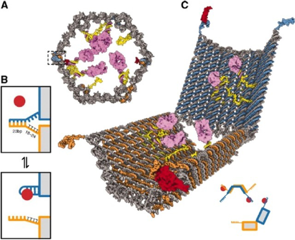
Figure 4. (a), (c)—opened and closed 3D models of the barrel structure, (b)—the aptamer-based lock. Reproduced from Douglas et al [36] with permission from AAAS.
Download figure:
Standard image High-resolution imageIn particular, including the sensitive aptamer-based lock required accommodations in the design, assembly, and verification phases.
As shown in figure 5(a), aptamers are short sequences of DNA that form some secondary structure which positions the charges and hydrophobic regions of the nucleotides to bind some non-DNA target molecule. By forcing some of an aptamers' ssDNA bases to engage in hybridization that competes with the binding state, one can create two metastable states whose equilibrium is controlled via analyte concentration and Le Chatelier's principle—where increasing reagent concentration will push a reaction to create more product in response.
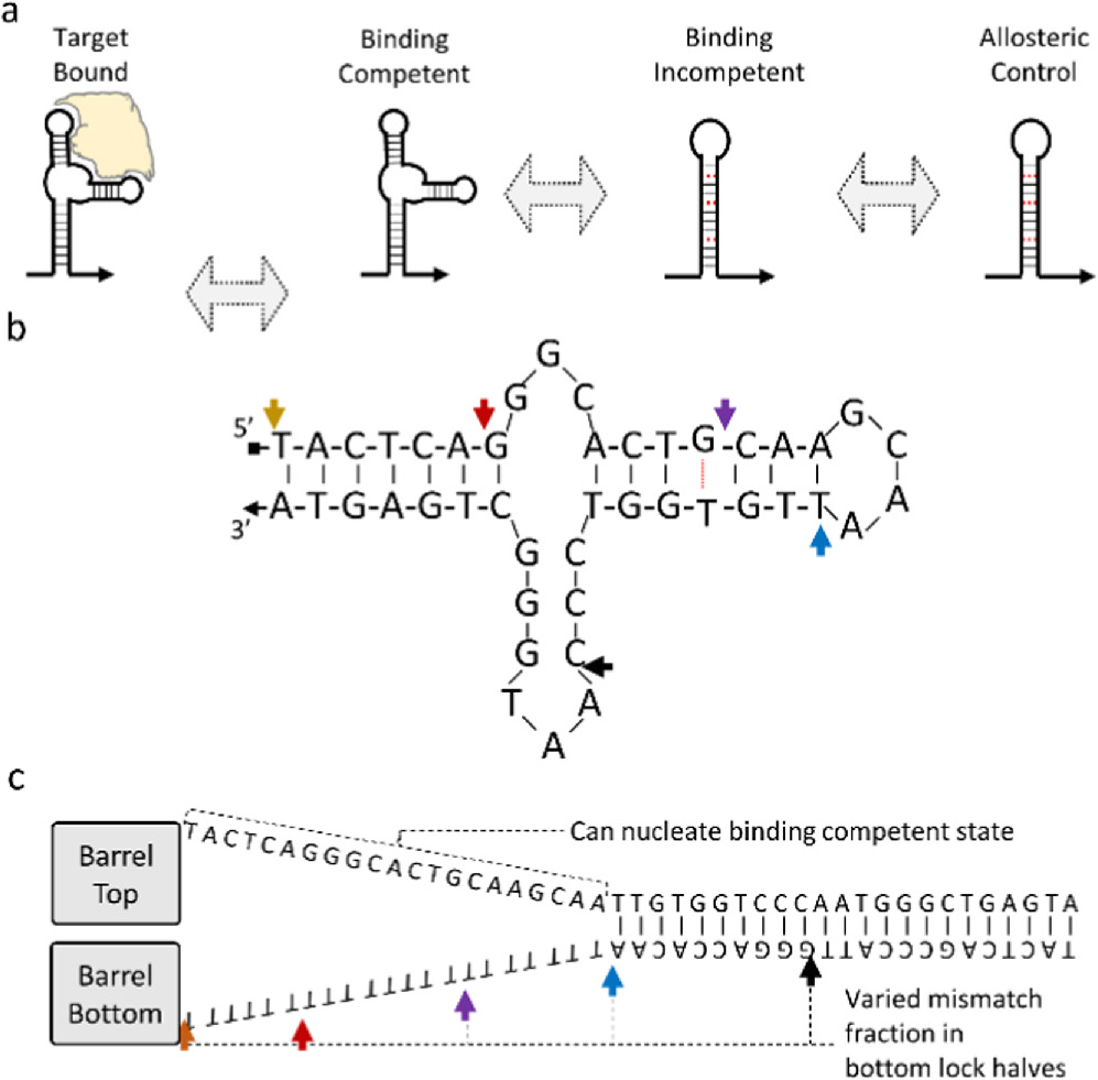
Figure 5. (a)—Schematic of how an aptamer sequence might be modified to sample binding competent and binding incompetent states, (b)—the aptamer originally reported by Green et al [48] (c)—competing dsDNA state, where the colored arrows in (b) and (c) represent the five different lock designs with varying levels of mis-matched polyT.
Download figure:
Standard image High-resolution imageAn aptamer can lock or move a DNA nanostructure. figure 5(b) shows the sequence of the aptamer used by Douglas et al and adapted from Green et al [48]. The arrows in figure 5(b) correspond to the five different versions of their lock, with the competing state design shown in figure 5(c). Each of the five lock designs varied the fraction of the aptamer sequence capable of nucleating the binding competent state.
This design, and most aptamer lock designs, are constrained in their energetics. The free energy of the dsDNA hybridization in the competing state must be more negative than the binding-competent state but have a higher free energy than the target bound state. Otherwise, the system would not be metastable, and would always remain locked or unlocked.
Douglas et. al manually explored the energetics to find a metastable state and avoid designs which would be fused closed and those which would spontaneously open. In this case, the aptamer locks, which could pop open, were also too weak to form the initial closed state in high yield.
This presents an informative systems engineering challenge. Douglas et al chose to address this problem with a threefold approach: first, by introducing guide strands to hold the structure closed at assembly; second, by removing the 'walls' of the barrel to allow payload loading without actuating the locks, and third, by developing a custom verification assay to measure individual opening and closing events.
These choices further altered the workflow, as Douglas et al introduced steps to remove the guide strands after the payload loading, and as they performed modeling estimates to assess whether the payload would have sufficient time to diffuse through the open barrel walls.
These workflow choices are why we chose this work as a case study. It emphasizes that the best workflow choice is the one which will work in the practitioners' own lab. Douglas et al's custom microbead assay for counting single barrel opening events, their use of live cells and flow cytometry, their choice of Fab' antibody fragment labeling chemistry, and their selection of purification for labeled AuNPs and Fab' fragments all point to the utilization of existing strengths in expertise and equipment.
One could imagine several counterfactual workflows which may, or may not, have succeeded.
- Design of a lock system reinforced with many more locks in parallel, requiring additional design work, and more intense verification to quantify the lock behavior in each design. It also would have increased the concentration of platelet-derived growth factor required to open the barrel.
- Design of a lock system using a stronger aptamer binding the same target, or a similar cell-surface protein target. This assumes one exists or assumes the resources could be dedicated to find one.
- Design of the nanostructure to act as a weaker entropic spring, or one with a neutral state closer to that of the locked barrel. This would reduce the energy required to hold the barrel closed but would likely reduce opening efficacy.
- Purification via some newly developed technique which separates the open and closed barrels. This would reduce the need for the guide strands and accommodate slightly weaker locks. However, even if possible, this choice would likely be dramatically less efficient than the guide strand approach.
Ultimately, any serious decoration project forces the practitioner to choose between a variety of such potential workflows. Navigating this space effectively is often underemphasized in the scientific literature, likely because including discarded workflow choices would be a tedious inclusion into supplementary documents.
One could imagine the same project utilizing very different workflow choices under different conditions. A collaboration with less flow cytometry expertise but more experimental and theoretical thermodynamics might have forgone a custom single barrel opening event assay for in-depth modeling and ensemble measurements. Similarly, a collaboration with significant expertise in synthesizing and testing libraries of DNA sequences for SELEX identification of aptamers might have developed a brute force approach to lock optimization. Ultimately, these counterfactual cases would have provided the scientific community with slightly different proofs-of-concept and would have had different probabilities of success.
The utility of thinking of project workflows in terms of phases, and of phases as groups of individual steps, is that it facilitates finding choices most aligned with the available resources and expertise.
2.3. DNA decoration decision making
Identifying and optimizing workflows, rather than individual phase-to-phase or step-to-step choices, allows prioritization for the success of the entire project. For example, both questions below could be asked of the same system.
'Should I perform (5+) multi-element decorations in a single pot anneal with a single purification, or should I divide my design into multiple single-element sub-structures with multiple purifications and combine them in an additional assembly step?'
And
'Should I pick the workflow that requires significant effort in developing purification, or the one requires significant effort in optimizing design and assembly conditions?'
Abstracting the former question into the latter enables evaluation based on available equipment and expertise. We liken this to balancing the weight of effort across the project, shown in figure 6, where the colored groups of phases represent possible effort tradeoffs. While it can take years of experience to develop an intuitive feel for how the weight of a project workflow is balanced, explicitly articulated planning is a more practical road to success.

Figure 6. Relationships in figures 1 and 2, emphasizing common tradeoffs in time-spent between tasks (white) as constrained by the functional requirements (red), where the diamond in the tradeoffs column is colored to emphasize which tasks are being balanced. The tradeoffs presented here parallel the example discussed above.
Download figure:
Standard image High-resolution imageEach of the following sections of this tutorial will provide a primer to an individual decoration phase describing the possible steps in that phase and what the constraints on those steps imply. The assembly section also includes the thermodynamics of sticky end decoration, and the verification section primer includes a short discussion of uncertainty and potential sources thereof.
3. Design
The first step of any decoration workflow is nanostructure design. The primary feature for this design process, and cornerstone of DNA nanostructure decoration, is addressability, i.e. the use of defined DNA sequences to place labeled elements at precise, predetermined locations on the structure. Locations may be singular, for example on an origami, or arrayed, in a tiling system with a lattice of identical locations. Tiling of non-identical units can be used to produce many unique locations, though at the cost of additional design complexity [49]. We note that this approach is limited: a system comprising thousands of oligomers folding into a single structure is likely to have sequences which, while technically unique, lack sufficient sequence orthogonality. The crosstalk between these strands will either reduce the effective concentration of the strands, potentially causing strand vacancies, or cause unintended strands to hybridize to incorrect parts of the structure.
This section will discuss designing an addressable position and a complementary functional element. Design choices include style of addressability, structure location, number of connections, element type, and element/oligomer connection chemistry. The related topic of thermodynamics of decoration will be addressed in the assembly section 4.1.
The spacing between functional elements is often critical to structure function. However, the sensitivity of function to spacing depends on the physical phenomenona at play and can vary dramatically. For example, distance variability will play a different role for a structure using Förster resonance energy transfer, FRET, than for one organizing ligands to bind to separate pockets on a biomolecule.
It is important to consider the accuracy and precision of programmed inter-element spacings. We define decoration accuracy as the agreement between a designed inter-element distance and the measured mean separation in an ensemble of nanostructures. The decoration precision would then be the standard deviation about this mean.
While these definitions are typical, they convolute structural fluctuations and inter-structure variability. Structural fluctuations vary the inter-element distance on the same structure over time. Inter-structure variability represents the distribution of mean inter-element distances between individual structures in a sample. To our knowledge few studies have deconvoluted these sources of variability, likely due to the difficulty of measuring inter-element distances over time for a statistically relevant number of individual structures. Recent modeling tools and metrology for dynamics structures appear promising approaches to adapt to this purpose [50].
It is not clear what the best achievable decoration precision might be, nor are there clear protocols on how to achieve it. However, recent studies can provide a general expectation for precision, shown in table 1. As they are also typically ensemble measurements, they could not capture fluctuations in inter-element distance over time or variations due to sample polydispersity. While the measurements are sufficiently different to make comparison difficult, they imply that interparticle spacing precision on the order of a nanometer is readily achievable.
Table 1. Example measurements of decoration precision in the literature. The quoted precisions are based on interparticle spacing measurements, not based on some absolute coordinate system, or relative to the nanostructure itself.
| Measured decoration precision | Method | References |
|---|---|---|
| ≈ 1 nm | Single interparticle spacing, via fluorescence lifetime | [7] |
| ≈ 3–6 nm | Single inter-particle spacing via AFM | [51] |
| <2 nm | Pitch measurement via AFM | [52] |
| ≈ 1–2 nm | Pairwise interparticle spacing via XRD | [53] |
Given the state of the art, we will discuss possible sources of inaccuracy and imprecision generally before we consider design in more detail.
3.1. Decoration placement
The most common tool for creating addressable locations on a nanostructure is the use of sticky ends, which are additional lengths of unpaired single-stranded DNA, ssDNA, which exit a structure. The functional element is labeled with ssDNA of complementary sequence to the sticky end on the structure. A key feature of sticky ends is that they do not benefit from the natural stoichiometric controls and cooperativity typical of origami - the target strand is not guaranteed to strand displace a partially complementary sequence incorrectly bound to the sticky end.
Best practice for sticky end driven decoration accounts for incorrect binding in two ways. First, the labeled element is only added after an initial purification to remove excess copies of the sticky end strand which could prevent binding. Second, both the sticky end strand on the nanostructure and the sticky end strand attached to the functional element are purified, typically via polyacrylamide gel electrophoresis, PAGE, to remove off-target sequences. Other approaches include using a high number of duplicate sticky ends on both structure and particle to ensure binding even if several positions do not bind appropriately. An alternative approach is direct labeling, in which the functional element is labeled with a strand that directly hybridizes to the nanostructure in the initial anneal without a facilitating sticky end. This technique is limited by both reduced flexibility and the thermostability of the functional element. However, direct label binding may result in higher yield during scale-up as it combines steps for excess staple purification and for excess functional element purification.
Note: direct labeling is incompatible with nanoparticles that require an excess of the linker modified strand, e.g. thiol/gold nanoparticle connections
Direct labeling is also incompatible with any anchor chemistry which cannot survive thermal or chemical anneal conditions.
Sticky ends are ubiquitous due to their modularity at the lab level: the same sequences are often used for multiple projects, reducing the upfront cost of expensive labeled oligomers. This also allows the location and types of functional elements to be easily exchanged within in a lab's library of raw materials. Section 3.5 will discuss sequence design for sticky ends, and the energetics of sticky ending binding will be discussed in section 4.1.
Sticky ends traditionally have spacer nucleotides between both the nanostructure and sticky end, and between the sticky end and the functional element, shown in figure 7. Generally, the longer the sticky end is, the more thermodynamically stable it will be, as discussed in section 4.1. Longer spacers will improve yield by minimizing steric and charge repulsion effects but, as shown in figure 8(b), longer and more flexible sticky ends will also have more freedom to move around the anchor point where the sticky end exits the origami.
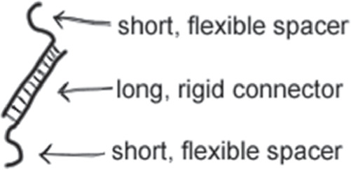
Figure 7. Anatomy of a sticky end connection.
Download figure:
Standard image High-resolution image
Figure 8. Schematics of (a) label connection at 5' or 3' position and subsequent binding, the blue line indicates the sticky end sequence and the red dot indicates linker chemical moiety, (b) particle motion and position as a function of the number of sticky ends, (c) common three sticky-end binding positions, (d) multivalent binding of particles to multiple structures, (e) desired binding, with each binding site occupied by one particle and undesired binding, with one particle occupying multiple binding positions.
Download figure:
Standard image High-resolution imageThe length of a sticky end will also play an important role in synthesis. Phosphoramidite synthesis yield is given by equation (1). This is more critical for sticky end strands than for typical staples or tile strands because the sticky ends must be purified, to remove off-sequence products. As material is lost in the purification process, and as chemical linkers are often necessary to connect to the functional element, these strands tend to contribute disproportionately to the cost of the structure.
Note: phosphoramidite synthesis can have a per base yield, or coupling efficiency, as high as 99.5%, this can result, for strands of 20 nt, in at least 10% of sequences having at least one error.
- Off sequence sticky ends or complementary labels can prevent binding, or otherwise hinder assembly. To ensure binding to the correct location, BOTH structure sticky end AND functional element label complement must be purified either by the manufacturer or the practitioner.
- Most manufacturers offer purification of synthetic DNA oligomers. The cost, yield, and purity of product will vary by manufacturer and purification technique.
Another relevant design factor in creating sticky ends is the anti-parallel hybridization of DNA. As shown in figure 8(a), whether the sticky end is attached in the 5' or 3' direction on the functional element and nanostructure can significantly change their binding geometry. As with the addition of spacers, there is some tradeoff between the site occupancy of functional elements and the closeness of binding, likely due to steric hindrance [52].
The number of sticky ends used to connect a nanostructure and functional element can change the position of an element relative to the structure, how much mobility it has around its average position, variation in that position over many copies of a structure, and the thermodynamics of the assembly. This is shown in figure 8(b), while a schematic of a typical sticky end labeling is shown in figure 8(c).
When using multiple binding sites, polymerization is possible, especially for NPs labeled with an excess of sticky end complements. In these cases, it is possible for two or more structures to bind the same particle or vice versa, as shown in figures 8(d) and (e). This is controlled by introducing the structure and element when one or the other is in a large excess. Unfortunately, this necessitates either lower structural yield relative to input reagent or purification and recovery of the excess reagent. As clear rules have yet to be determined for predicting polymerization in these systems, some level of optimization is anticipated for most decoration projects.
While we will describe measuring yield of a desired structure in section 6, it is worth discussing design features that can contribute to improved yield. Relatively few studies have been published systematically examining the site occupancy of functional elements, likely due in part to the expansive design space [51, 52]. Relevant factors include inter-element distance, number of sticky ends on the element, size of the element, number of sticky ends on each anchor patch, and the shape of the nanostructure surface.
Work from Ko et al indicates that for biotin anchor positions binding streptavidin-coated functional elements, that three anchor positions per particle was sufficient for greater than 90% site-occupancy yield. This site occupancy dropped to below 75% for very densely spaced particles. Takabayashi et al [52] used 15 nucleotide sticky ends and tested the role of inter-element distance and number of binding sites. They examined 1, 2, and 4 binding sites, and found a yield of > 97% average site occupancy. They were able to mitigate yield loss due to reduced inter-element distance by interspersing two different sets of sticky end sequences, indicating that single particles bound to multiple binding sites was the primary mode of failure. Their theoretical analysis indicated an asymptote in site occupancy as a function of number of anchors per binding site and suggested 5 anchor positions as a reasonable maximum.
While the ideal arrangement of sticky ends for any given application must still be optimized, 3–5 anchor positions is a common place to start.
3.1.1. Sticky end positioning
As shown in figure 9, the first step in accounting for the exact X, Y, and Z position of an element follows the simple geometric rules, and depends on the number and types of linkers. Though this is complicated by variability in the internal crossover angle, see figure 12
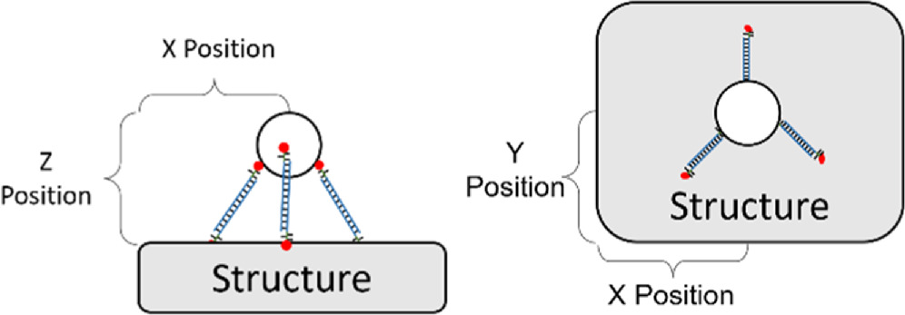
Figure 9. Relationship between particle X, Y, and Z position relative to the positions of the sticky-ends on the structure.
Download figure:
Standard image High-resolution imageIn theory, a practitioner can place a sticky end at any base position of a DNA nanostructure, within the resolution determined by the 0.34 nm base pair spacing along the double helix. However, the location of a sticky end is further constrained by choices made in the design of the nanostructure. The first constraint involves the stability of the sticky end's connection to the rest of the structure. While, to our knowledge, there have been no studies on stability as a function of the length of the anchor to the structure, or associated temperature dependence, it is a generally accepted rule that the sticky end should have at least 5–7 nucleotides, nt, of base pairing uninterrupted by a crossover. This is illustrated in figure 10.
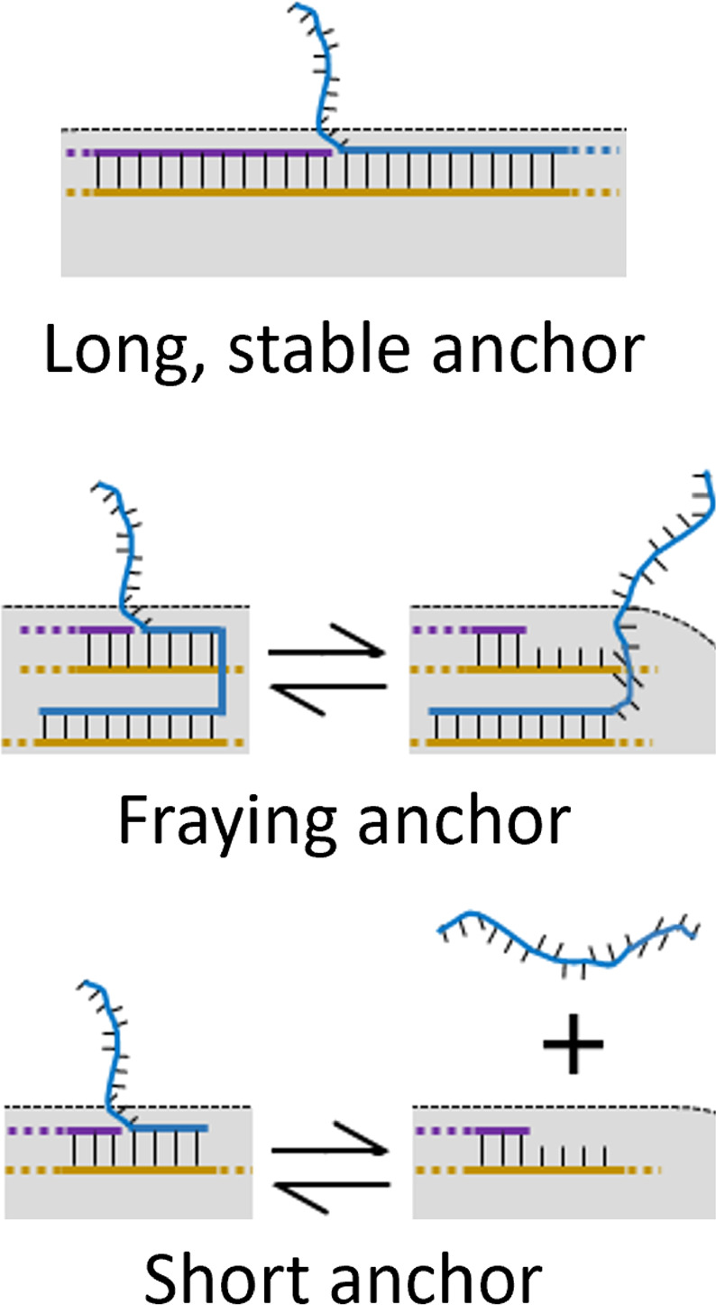
Figure 10. Schematic of how anchor length can result in sticky-end variability. Reproduced from Majikes et al [2].
Download figure:
Standard image High-resolution imageThe second constraint arises from the rotation of the helix. The sticky end will exit the structure at the physical location tangential to the minor groove position for the last nucleotide in the structure, which will rotate around the helix in 3D [54]. Care should be taken to confirm that a sticky end will exit the structure in the desired direction and not point into the structure or exit in the wrong direction. Many computer-aided design (CAD) tools have visual indicators for the rotational position of the minor groove of the helix. These functionalities vary between CAD tools but are a useful feature with which to familiarize oneself.
The process or determining the orientation at a particular base is illustrated in figure 11. One may calculate the exit direction for the sticky end via the right-hand rule combined with the direction of the staple, the direction of the nearest crossover, and the helicity of dsDNA. This can be done by pointing the right-hand-thumb in the 5'→ 3' direction and the index finger initially in the direction of the crossover. As the hand moves along the dsDNA, the fingers should curl at ≈ 0.598 rad per nucleotide (34.3 ° per nucleotide) in the 3' direction. This is approximately 3π/2 rad (270°) for every 8 nucleotides.

Figure 11. Using the right-hand rule to estimate the direction of an arbitrary base relative to the plane of a structure. Reprinted with permission from Majikes et al [2]. Copyright (2021) American Chemical Society.
Download figure:
Standard image High-resolution imageOther constraints include the skew of the crossover junctions, and deformation from internal or external stresses. The presence of neighboring sticky ends may also present topological limits to the length of neighboring staples. Additionally, the shape of a 2D structure can be different in solution as compared to on a surface [55].
While these constraints limit the exact positioning of a sticky end on the structure, they do not necessarily constrain the relative distance between sticky ends, or sets of sticky ends, in the same structure. This, and the lack of explicit studies on the limits of decoration precision make engineering for a predetermined positioning on the first try non-trivial. Often an iterative 'assemble-measure-and-modify' approach is taken, in which it is assumed that the initial predictions of functional element locations will be inaccurate.
3.2. Decoration accuracy
Few studies have reported designed versus measured intended inter-element distances, so there is not, to our knowledge, best practice for achieving a desired spacing in a completed structure. We can, therefore, only describe useful design concepts and give general recommendations. For systems where a highly accurate initial guess is required, we recommend iterative design, and rough structure simulation (finite element [17] or coarse grained [14, 15, 56]) followed by molecular dynamics simulations [57]. For particularly demanding applications, planning alternative versions of the binding locations and strand sequences in advance may be prudent.
The primary source of decoration inaccuracy is in predicting the exact dimensions of a DNA nanostructure prior to fabrication. As shown in figure 12 the idealized shape of a structure as seen in CAD tools fails to account for the structure and angle of crossover junctions. Beyond what is shown in figure 12, Holliday junctions, the biological analogue of the crossover junction, have a small skew, which would be out-of-page in figure 9, and may flex in that direction to minimize charge density [58]. An in-plane angle of π/3 rad (60°) is a commonly accepted value in biological contexts [58, 59]. This angle is likely to be lower in DNA nanostructures, and may vary between designs, particularly for 2D and 3D structures, and quantification of these angles in origami or other DNA nanostructures has been a subject of few publications, typically in the context of mechanical properties [60], ion dependent reconfiguration [61, 62], novel characterization [63–65], and bistable physical isomorphs [66, 67].
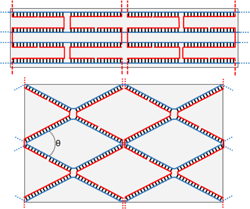
Figure 12. Idealized versus relaxed crossover patterns and estimated relaxed dimensions. Note that the relaxed angle in this figure appears exaggerated as the line form of representation has a lower aspect ratio than real DNA.
Download figure:
Standard image High-resolution imageIt is worth noting that both the schematics in figure 12, and in most CAD tools, can visually imply larger spacings than occur practically. This is because the aesthetics of traditional line representations of dsDNA under-represent the width of the helix. A more accurate, but more cluttered, representation in figure 12 would have helix widths consuming approximately half of the empty space in the lattice.
Other sources of systematic inaccuracies in a designed inter-element distance may include an inaccurate mean functional element size, and charge repulsion for large or highly-charged functional elements.
Given the lack of in-depth studies on this topic, practitioners often take an iterative 'assemble-measure-and-modify' approach, in which it is assumed that the initial predictions of function element locations will be inaccurate.
3.3. Decoration precision
3.3.1. Inter-structure variability
For particles, the largest source of inter-particle spacing variation comes from variation in particle size. As shown in figure 13, the distribution of particle sizes, referred to as polydispersity, maps intuitively onto the inter-particle distances. It is for this reason that we highly recommend either characterizing all NP size distributions prior to decoration or purchasing NPs that include size distribution quantification in their quality control documentation.

Figure 13. Interparticle distance as a function or variability in radius where d4 < d2 < d1 < d3.
Download figure:
Standard image High-resolution imageGenerally, equation (2)–(4) provide the shortest distance between two particles bound to an origami with the assumption of a Gaussian particle radius distribution, neglecting binding height variability, and other factors, shown in figure 14. Note that dhyp is the distance between particle centers and is equal to the dactual+ra
+rb
. To address the more common log-normal NP radius distribution we would recommend Monte Carlo simulation. We discuss uncertainty propagation more generally in section 6, though this is a useful and specific example. We will use the notation where  refers to uncertainty on some value
  represented by the standard deviation of the distribution of multiple measurements of
  In this case
  would likely come from the shape of the structure and the crossover junction angle, while
  would be from the polydispersity of the particle a and b ensembles.


Figure 14. True interparticle distance as a function of ideal distance and difference in radius.
Download figure:
Standard image High-resolution imageIn this description ddesigned is the designed distance between particle attachment points, dhyp is the distance between particle centers, and dactual is the distance between particle surfaces. If this model is accurate, we can recast the uncertainty in the true interparticle distance as a function of the particle radii and uncertainty in their radii.
![${\sigma }_{\mathrm{actual}}=\sqrt{{{d}_{\mathrm{hyp}}}^{2}\left[{\left({2d}_{\mathrm{designed}}^{2}\tfrac{{\sigma }_{\mathrm{designed}}}{{d}_{\mathrm{designed}}}\right)}^{2}+{\left(2{d}_{z}^{2}\tfrac{{\sigma }_{z}}{{d}_{z}}\right)}^{2}\right]{+\sigma }_{a}^{2}+{\sigma }_{b}^{2}}$](https://content.cld.iop.org/journals/0957-4484/35/27/273001/revision3/nanoad2ac5ieqn6.gif)
For sensitive applications, such as FRET lifetime engineering [7], or for more complex distributions of particle radius, we suggest Monte Carlo simulation of distances.
The National Institute of Standards and Technology provides an online Monte Carlo simulation tool, the NIST uncertainty machine [68]. Documents for best practice in expression of uncertainty include the international Guide to the expression of Uncertainty in Measurement, or GUM [69].
A less easily quantifiable source of variability is degenerate binding positions for particles with a random distribution of sticky-ends, or other anchor modifications, across their surface. The three bound particles in figure 15 all would be expected to have roughly the same free energy of binding if one neglects electrostatic repulsion and the loss of nanoparticle translational entropy from left to right. One would therefore expect a distribution of those possible binding positions in any fabricated sample.
Variability between nanostructures in a single sample can also be ascribed to assembly errors, either in the binding of the functional elements, or in the structural DNA maintaining distance between those elements.
3.3.2. Structural fluctuations
Motions within individual structures over time are a final source in inter-element distance variation. There are three major sources: slack in functional element binding, fluctuation in crossover shape, and overall structural flexibility.
As we discussed in section 3.1, small spacers are often left between a structure or functional element and its linking modifications or sticky ends. These spacers can improve site occupancy [50, 59], however, they also allow functional elements to float around the center of the binding site, shown in figure 8(b).
Figure 15. Height variability due to locations of binding strands on nanoparticle.
Download figure:
Standard image High-resolution imageThe angles made between strands participating in a crossover junction are not completely static, figure 16. It has been shown in the literature that they can be bistable and jump between equivalent parallelograms [67]. While these transitions are rare unless they are explicitly designed in, it is reasonable to expect that the angle of the crossover junctions to fluctuate slightly in solution, and that these fluctuations cause slight variations in the distance between functional elements. Like the exact value of the crossover junction angle, this is likely to vary between structures, particularly between 2D and 3D designs.
Figure 16. Variation in the angle of the crossover shifting the aspect ratio of a structure, as the average θ changes, the overall shape of the structure can change. Note that the relaxed angle in this figure appears exaggerated as the line form of representation has a lower aspect ratio than real DNA.
Download figure:
Standard image High-resolution imageFinally, structural bending will play a role in distances between functional elements, particularly for 2D structures. In the direction of the helices, 2D structures are highly rigid. However, the crossover junctions may act as hinges in the direction perpendicular to the helices. 2D structures therefore have high and low persistence lengths in the direction of, and perpendicular to, their helices [60, 70]. Most studies measuring interparticle distance have either used the highly rigid 3D six helix bundle or placed particles on the same helix of a 2D origami. As such, there is limited quantification of this phenomena, although bending has been used in conformational sensors [71].
3.4. Types of functional elements
A comprehensive list of functional elements that have been, or could be, attached to DNA nanostructures is beyond the scope of this tutorial, though we suggest the following review [28]. Similarly, there are reviews which cover specific families of functional elements in more detail, e.g. proteins [72] and aptamers [73]. Here we list common functional elements, linker moieties, and chemical modifications to DNA. Table 2 details common functional elements that have been published frequently.
Table 2. Common nanoscale functional elements, typical linker chemistry, and compatibilities. Many of those listed here can be implemented using commercially available functional elements and linkers.
| Element | Function | Common linkers | Notes | |
|---|---|---|---|---|
| Peptide | ||||
| Molecules | 2–50 amino acids | Binding biomolecules | Click chemistry | Can thermally anneal |
| <103 g·mol−1 | Binding small molecules | NHS ester | Can chemically anneal | |
| <1 nm | Can spin-filter purify | |||
| Typically, non-toxic | ||||
| Protein | ||||
| >50 amino acids | Binding biomolecules | Click chemistry | Toxicity depends on protein | |
| >5 × 10⁴ g·mol−1 or more | Binding small molecules | NHS ester | Denature both chemically & thermally | |
| >3–10 nm | Enzymatic catalysis | |||
| Biological interface | ||||
| Covalent modifications (Fluorophores, Quenchers) | Fluorescence | Usually as part phosphonamidite synthesis, or post synthesis NHS ester addition | Can thermally anneal | |
| Hundreds of g.mol−1 <1 nm | Toxicity depends on modification | |||
| Aptamers (15–90) nucleotides, nt (6 × 10³ to 3 × 10⁴) g·mol−1 ≈ 3 nm | Binding biomolecules | None needed | Can thermally anneal | |
| Binding small molecules | Toxicity depends on aptamer, generally low immunogenicity | |||
| Lipids bilayers or vesicles of varying size | Separate chemical | Cholesterol | May non-specifically interact, particularly | |
| environments | with hydrophobic surfaces and molecules | |||
| Nanoparticles | Gold nanoparticles (AuNPs) | Quenching fluorophores | Thiol | High mass contrast (good for EM, gel purification, gradient ultra-centrifugation) |
| Plasmonic coupling | Alkyne | Toxicity depends on stabilizing ligands | ||
| Seeding metal growth | Poly-T | Thermostability depends on stabilizing ligands | ||
| Quantum dots (QDs) | Fluorescent | Depends on outer shell material | High mass contrast | |
| Typically toxic | ||||
| Semiconducting nanoparticles | Tuned bandgap (Usually, to absorb light and transfer energy to some other element) | Silane | High mass contrast | |
| Can be toxic | ||||
| Iron oxide nanoparticles | Magnetic separations | Multi-layer ligand addition | High polydispersity | |
Table 3 lists common linker moieties. It should be reiterated that it is far from exhaustive. The protein bioconjugation literature is deep, with a wide variety of strategies for covalent linkages [74]. We refrain from discussing them in detail as many require development of more specific skills than those new to DNA nanotechnology might be expected to have. The aptamers discussed in table 2 are sequences of nucleic acid that form a 3D structure which binds some target and can be used as a linker without requiring a chemical modification.
Table 3. Common commercially available linker moieties, their approximate size, as well as their typical constraints and uses. Other moieties such as silanes, acrydites, amines, etc are often also available, but to our knowledge are more commonly used in the biochemical community.
| Name | Chemical structure | Size | Notes | Commonly used for |
|---|---|---|---|---|
| Thiol | −S | <1 nm | Forms di-thiols | Gold |
| Non-covalent protein binding | Biotin (Streptavidin Binding) | ≈ 5 nm | Streptavidin is tetravalent | Proteins and large particles |
| Thermally denatures | ||||
| Digoxigenin (Antibody Binding) | ≈ 10 nm | Most antibodies are divalent | Proteins and sandwich assays | |
| Thermally denatures | ||||
| Covalent bonding | Click Chemistry (copper catalyzed alkane and azide cycloaddition) | <1 nm | Requires protection for proteins (typically an intercalator for metal ion catalyst) | Any appropriately labeled molecule or particle |
| NHS ester and amino groups | <1 nm | Reagent NHS esters are stable 4 to 8 h. in water | ||
| Non-specific surface binders | Cholesterol, Alkyne, etc | <1 nm | Lipids, proteins, gold surfaces |
Table 4 shows common modified backbones that might be used in a structural context. Numerous other commercially available modified bases exist to support biochemical assays for applications ranging from fluorescent reporting to nuclease resistance and photo crosslinking. See the cited review for a more thorough description of modified bases relevant to biological applications [39].
Table 4. Common modified DNA backbones for structural applications.
| Name | Chemical structure | Description |
|---|---|---|
| Deoxyribonucleic acid (DNA) |
| Standard DNA, bases attached to a sugar-phosphate backbone |
| Peptide nucleic acid (PNA) |
| Nucleic Acid in which the sugar-phosphate backbone is replaced with a peptide backbone. They are more nuclease resistant, and have less charge |
| Bridged nucleic acid (BNA) |
| A DNA backbone where the 2 and 4 carbons are connected by a bridge where X can be a variety of atoms |
| This prevents the base from rotating, which in turn reduces the loss in entropy on hybridization, stabilizing the dsDNA state | ||
| Locked nucleic acid (LNA) |
| A class of BNA in which the bridging moiety comprises a carbon and an oxygen |
| Abasic DNA |
| A nucleotide without the nucleobase, preventing base pairing |
| Often used as a spacing motif |
3.5. Sticky end sequence design
The thermodynamics of DNA hybridization will be discussed in section 4.1, however the choice of DNA sequences in the context of design merits discussion. For DNA origami, the staple strand sequences are determined by where they bind to the scaffold. Little to no manual sequence design is necessary for origami staple strands. Sticky ends are often the only sequences that a practitioner will design.
As the number of sticky ends, or strands generally, in a system increases, so to does the probability of unintended complimentary interactions. For small numbers of sticky ends less than 30 nt in length, random sequences are often sufficient. However, as decorated DNA nanostructures increase in complexity, more rigorous design will be required.
For single digit numbers of sticky ends, this often involves manual checks for stable hairpins and for stable, but undesirable, complementarity between supposedly orthogonal sticky ends. Hairpins on a sticky end can dramatically reduce hybridization kinetics. Unintended stable complementarity between strands can reduce their effective concentration or result in polymerization. In both cases, the kinetics of assembly are slowed [75].
Numerous webtools exist to evaluate hairpins and partial strand complements [76–80]. While most strands will have some hairpin interaction with themselves, or partial complementarity with other strands, many of these interactions will be unstable at or above room temperature.
One trick for manual sequence design and optimization is to use only three of the four nucleobases on each strand, e.g. one sticky end would only be comprised of the letters A, G, and C while its complement would only be comprised of T, C, and G. In a strand with only A, G, and C, the A bases cannot contribute to hairpin stability as they have no T bases to pair with. Similarly, two orthogonal strands which are only comprised of T, C, and G can only have partial complements between their C and G bases. However, this does have the disadvantage of reducing the number of possible sequences.
To our knowledge, there have been no studies on the optimization of large numbers of sequences in the decoration context. However, there is significant literature on sequence design for tiles and junctions [81], algorithmic assembly [82], strand displacement [75, 83, 84], and data storage. This includes tools to minimize unintended complementarity in silico, which could presumably be easily adapted to sticky end design [81, 85, 86].
4. Decoration assembly
Assembly of DNA nanostructures inherently involves ssDNA to dsDNA hybridization reactions. These reactions are mostly performed across an energy gradient, typically via thermal anneals.
We begin with the thermodynamics of plain DNA hybridization before addressing the thermodynamic considerations of sticky end binding. The energetic contributions associated with the topology changes in DNA nanostructure folding are still an open challenge and are beyond the scope of this tutorial.
4.1. Plain DNA hybridization and melting thermodynamics
Control over the melting temperature and sharpness of the melting transition are two useful but relatively underutilized design degrees of freedom. These parameters are determined by the energetics of hybridization, which can be modeled to provide a melting temperature, Tm, defined as the point at which half of the strands are released. It is also possible to determine, more or less accurately, the width of the melt curve. The degree of accuracy depends on how similar the system is to ssDNA ↔ dsDNA hybridization.
In some cases, one need only know the approximate stability of some sequence at room temperature that singly connects an element to a nanostructure. In others, a practitioner might model the energetic contributions to optimize the sticky end sequences: modifying sequence length may allow creation of structures with minute shifts in element location or may remove undesirable cross-hybridization with other strands or may simply shorten strands and reduce costs. In other projects, such modeling is critical, e.g. when engineering multiple meta-stable binding states, the population of which is controlled by temperature, pH, or analyte concentration.
For many applications, existing predictive webtools [76–78], or even empirical equations relating Tm and GC content may be sufficient. For those, it is enough to remember trends in length, GC content, concentration, and salt content, depicted in figure 17, and that unimolecular reactions like hairpins are more stable. For those practitioners who will need to model the hybridization in their own system we introduce the relevant nuances below.
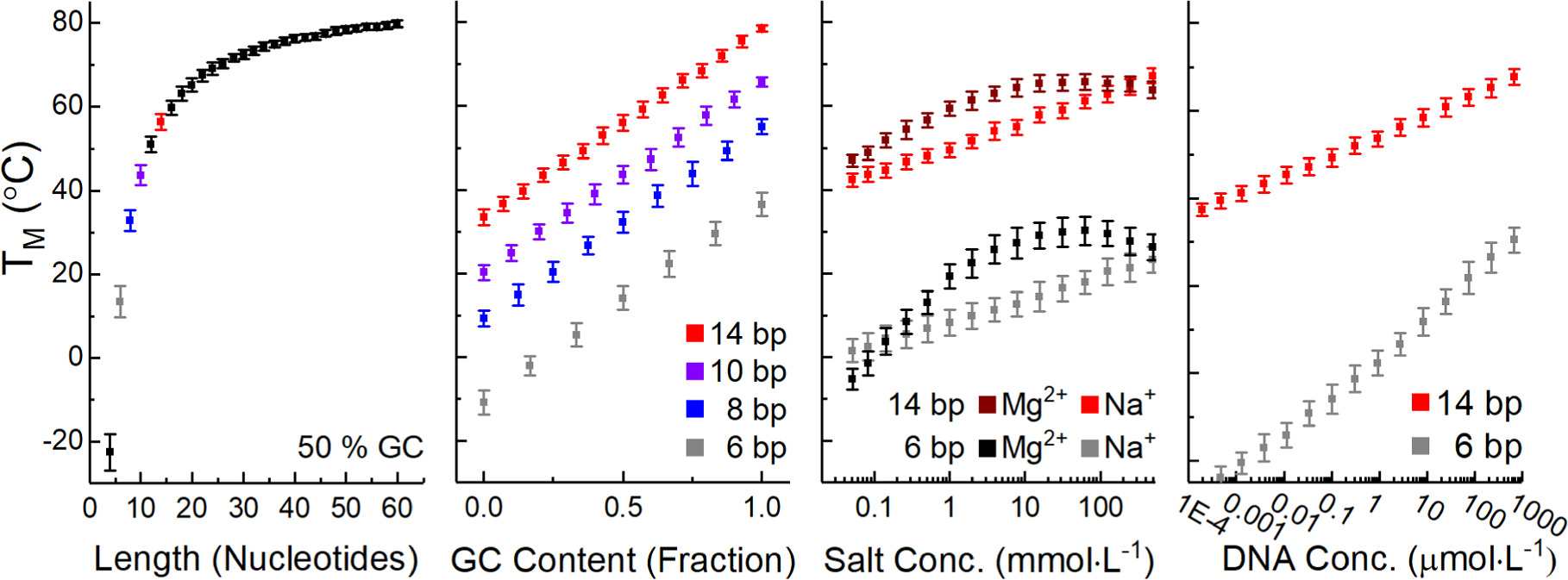
Figure 17. Nearest neighbor model predicted Tm as a function of oligomer length, fractional GC content, and salt concentration. Unless otherwise indicated in the x axis all predictions in this figure used a dsDNA concentration of 40 μmol·l−1, a GC content of 50%, and 1 mol·l−1 NaCl. Uncertainty bars represent a single standard deviation across the Tm of 50 randomly generated sequences. The error bars represent a single standard deviation across the Tm of those 50 sequences. The data point colors are set to be consistent between subplots.
Download figure:
Standard image High-resolution imageIn B-form DNA the major factors controlling hybridization stability and melting temperature, Tm, are sequence, length, salt concentration, and strand concentration. The main driver of hybridization is the hydrophobic π–π stacking between bases up and down the helix, with minor contributions from hydrogen bonding between base pairs and electrostatic repulsion. The shorter a strand is, the more the unfavorable interaction between the terminal bases and water contributes relative to favorable interactions between bases within the helix. Similarly, as guanine and cytosine bases have more favorable base stacking, a higher GC content will result in a more stable helix. Salts release the water molecules bound to the phosphate backbone and shield its negative charge, entropically increasing stability. Finally, increasing strand concentration shifts equilibrium to hybridization at higher temperatures, as one would expect via Le Chatelier's principle—where increasing reactant concentration will push a reaction to create more product in response.
Typical thermodynamic prediction uses the van't Hoff relation by identifying the form of the equilibrium constant and the predicted ΔH and ΔS for a sequence under specific conditions, then solve for the fraction, or concentration, of ssDNA. Prediction of ΔH and ΔS can be done through the nearest neighbor, NN, model. Here we use the NN parameterization presented by Santa Lucia et al [87]. The conditions under which these models have been parameterized do not perfectly translate to the those present for DNA nanostructures, but they do provide a useful foundation from which to build.
To find a predicted ΔH and ΔS, proceed through the sequence in neighboring sets of bases and add up the energetic contributions for the terminal bases and each set of neighbors. For ATGCAT, one would add ΔH and ΔS pairs for A+T, T+G, G+C, C+T, and A+T, then add the appropriate energetic penalties for termination in A and T. The summed ΔH and ΔS would then be adjusted for salt concentration [88] or other DNA motifs. This model assumes ΔH and ΔS are temperature independent, i.e. they neglect change in heat capacity ΔCp. While this is an oversimplification [89], it is sufficient for our purposes as the ΔCp primarily increases the asymmetry of the melt curve and does not significantly shift the Tm.
The van't Hoff relation is given in equation (5), where [ ] brackets indicate concentration relative to the standard concentration (1 mol·l−1), T is the temperature, and R is the gas constant.

For unimolecular reactions the equilibrium constant is given in equation (6) where [ssDNA] is the concentration of denatured ssDNA molecules and [dsDNA] is the concentration of hybridized dsDNA. As most melt curve measurements do not give absolute concentrations, this is often rewritten in terms of the fraction of DNA that has melted, fss
. In such cases ![$\left[{ssDNA}\right]={f}_{{ss}}* \,\mathrm{conc}$](https://content.cld.iop.org/journals/0957-4484/35/27/273001/revision3/nanoad2ac5ieqn7.gif) where the term conc describes the total DNA concentration. It should be noted that this term is still relative to 1 mol·l−1, and is thus unitless, which ensures that
where the term conc describes the total DNA concentration. It should be noted that this term is still relative to 1 mol·l−1, and is thus unitless, which ensures that ![$\left[K\right]$](https://content.cld.iop.org/journals/0957-4484/35/27/273001/revision3/nanoad2ac5ieqn8.gif) is unitless regardless of reaction form.
is unitless regardless of reaction form.
For unimolecular reactions, the absolute concentration terms cancel to give equation (6)
The Tm is defined by the point at which fss = 0.5. Note a common, but poor, assumption is that this temperature can be found at the peak of the derivative of the melt curve as function of temperature [90].
If neither strand is in excess, the Tm is given by equation (8), although this is often not the case for DNA nanofabrication systems.

If an excess is present, it is useful to define conc as the concentration of the limiting reagent, as this is also the maximum possible dsDNA concentration. The fractional excess relative to the limiting reagent can then be used to give equation (9). For example, if two complementary strands are at concentrations of 5 nmol·l−1 and 50 nmol·l−1, there would be a 10× fractional excess and conc would be 5 nmol·l-1.
When building one's own predictions, it is advisable to note the sign conventions used for additional motifs and to compare several 'control' predictions to existing prediction webtools [76–78]. The scientific literature is not uniform in reporting in terms of energies of melting or of hybridization, making it easy to make a sign error that results in non-physical predictions.
To illustrate the general trends of DNA melting, we plot modeled Tm as a function of length, GC content, salt concentration, and DNA concentration, as modeled by [86]. All data points in figure 17 represent 50 random sequences, even if there are fewer than 50 possible sequences for that combination of length and GC content.
The Tm is most sensitive to DNA length followed by GC content, and salt concentration. The Tm dependence on concentration varies significantly between more and less stable strands. Divalent salts are more effective at charge screening than monovalent salts, and in the typical concentration range, (0.1–50) mmol·l-1, Mg2+ increases stability more than Na+. Generally, the Tm of a less stable strand will shift more for the same change in length, GC content, salt concentration, or DNA concentration than a more stable strand, as seen in the last two panels of figure 15.
While there are not NN model corrections for polyamine multivalent salts, e.g. spermine, putrescine, spermidine, etc, or oligolysine both the former [91–93] and the latter [94, 95] can dramatically increase the Tm, and can protect DNA from damage in biological systems.
4.1.1. Example use cases
After purification of excess staples, or of excess functional elements, one would anticipate a lower reagent concentration, and thus lower stability, and thus a lower shelf-life. Energetic estimates of melting temperature can help to predict whether one's sticky ends will stay hybridized under application conditions. This is especially useful for cases where structures are used in low ionic strength conditions. Estimates of melting temperature are also useful to troubleshoot weak connections between structures and functional elements, and in ensuring undesired cross-hybridization is too weak to interfere with assembly [96].
4.2. Hybridization with multiple sticky ends
The binding of a functional element can be much more complex than typical hybridization. The functional element can only decouple from the structure if all its sticky end connections are melted. The probability of an element being connected, fc , is the probability that each of its N sticky end connections are melted, described in equation (10).

These equations can be rearranged to give the decoupling Tm, at which Fc = 0.5, as a function of N, as shown in equation (11) [97].
In figure 18 we plot the probability of disassociation for functional element decoupling for a single random 14 nucleotide sequence as a function of number of sticky end connections. As the number of sticky ends increases, so too does the sharpness and Tm of the melt curves.

Figure 18. Predicted functional element decoupling curve for a sticky end of random sequence of 14 nt at 40 μmol·l-1 functional elements and 1 mol·l-1 NaCl as the number of sticky end sequences increases from 1 (black), 2 (blue), 3 (purple), to 4 (red). As each curve is a single prediction, there are no uncertainty bars.
Download figure:
Standard image High-resolution imageUnfortunately predicting the Tm and melt transition breadth is much more complicated than equation (11) and figure 18 may imply. The NN model assumes that the final dsDNA will have 3 rotational and 3 translational degrees of freedom. However, when multiple sticky ends connect a single functional element, they will have fewer degrees of freedom. By equipartition theorem, one would anticipate a loss in entropy for each lost degree of rotational or translational freedom. When performed carefully this type of modeling can even predict complex binding topologies such as those considered by Dreyfus et al [97]. There are also enthalpic interpretations of the increased binding stability of ssDNA with ssDNA anchored to particles that may be relevant [98].
This additional means of control over Tm and transition width can provide options in nanostructure design. In the context of figure 18, elements bound to a nanostructure with the same Tm may be held closer or further from the structure depending on the number and length of the sticky ends. Similarly, as missing staples in an origami are not improbable, the number and length of sticky ends could be tuned to either minimize loss in decoration precision, e.g. figure 8(b), or to ensure that origami with missing staples are unable to bind the functional element at all.
This source of energetic control is particularly relevant for controlling nanostructure or functional element conformation, as in the case study in figures 4 and 6. It is possible to re-arrange equations (5), (7), and (10) to solve for fraction of aptamers held or released as a function of target molecule concentration.
The depth to which a practitioner will model the thermal behavior of sticky end connections will depend on the complexity of the system and how important its behavior is. While this type of modeling is not currently common place for experimental design, we anticipate it becoming a useful tool for designing the free energy landscape of multiple states to create dynamic motion [10].
Example cases: In engineering plasmon resonance, large particles must often be brought into proximity, taking advantage of multiple connections to use shorter strands to bring the particles in closer proximity cold be valuable. For rapid reconfiguration of a system at a specific temperature, controlling the breadth of the transition between states will also be vital. In the first case simple modeling may confirm the stability of the shorter strands as a function of number of connections, while in the latter more in-depth modeling may be necessary.
Given the complexity of these systems, any general rule would have a broad array of exceptions. However, in most cases one could rank the factors changing stability by magnitude, from largest to smallest, as follows:
- Longer sticky ends
- Higher GC content
- Increased number of binding sites (# of sticky ends)
- Higher salt concentration
- Additional degree of freedom penalties
- Higher functional element (or DNA) concentration
As a rule, the Tm of a bound functional element will be higher than its sticky end's NN model predicted Tm, except in cases where steric hinderance destabilizes the binding.
4.3. DNA nanostructure annealing
Annealing protocols ensure the molecules can explore a large free-energy landscape comprising a variety of configurations and hybridization states, steadily progressing to the lowest energy state, which is presumably the target nanostructure.
DNA hybridization is a reversible reaction: above the Tm, hybridized dsDNA is unfavorable, and below the Tm that states are increasingly favorable. However, at lower temperatures the kinetics of a DNA strand finding an optimal binding position are much slower than the kinetics of suboptimal or defect positions. There are many possible unique, undesired, binding positions in a DNA nanostructure that compete with the target structure, which leads to a relatively high probability of defective binding of the wrong strand, i.e. site poisoning.
In DNA nanostructures, particularly DNA origami, each hybridization reaction is unique and energetically reinforces its neighbors, making the assembly process a cooperative one. As a result, annealing protocols often only require mixing all the DNA sequences in a single vial, using temperature to fully de-hybridize the DNA, and then slowly cooling down the mix. This is often sufficient to get decent structural yields; 60% to 80% with minimum effort. Early anneal protocols were as simple as polystyrene boxes filled with boiling water in which the vials were left overnight. Many protocols for annealing have been developed ranging from isothermal [21, 99], to those using chemical rather than thermal energy [100], to speculative applications of mechanical denaturation [101].
However, as structures get larger there is a higher probability of unwanted sequence crosstalk, and as they become more complicated, particularly 3D DNA origami or DNA bricks [20], the kinetic traps become more problematic. In such cases, optimization of annealing protocols becomes more important and more complex.
In complex 3D origami or large DNA bricks assemblies, attention should be paid to the design itself and to ensuring nucleation occurs at the center of a structure. Failure to do so could result in kinetically trapped defective structures if the outside of the structure is fully folded and prevents diffusion of staples to its center. Another issue to consider is the thermal, or chemical, stability of the functional element.
We encourage the practitioner to treat annealing as an optimization step—a fine-tuned anneal protocol can improve yield whether through higher reactant oligo concentration or a slower anneal rate. However, if several initial anneals do not result in a measurable amount of desired structure, it is probable that no such protocol exists. In such cases the practitioner should consider either going back to the design stage, or (for tile-like systems) performing stepwise combination of reactant strands to troubleshoot which interactions are not hybridizing as expected.
4.3.1. One pot versus multi-step assemblies
While purification occurs after assembly, it is not uncommon for workflows to have multiple annealing and purification steps. This is often due to the thermal and chemical compatibilities of functional elements and the removal of excess reagent strands. These excesses can interfere with verification, and with any future annealing steps in the workflow. It should be assumed that each separate assembly phase will be accompanied by a purification phase.
As each assembly and purification iteration reduces the final yield, it is desirable to choose functional elements and chemical linkers whose compatibilities minimize the total number of assembly and purification steps.
5. Purification
Purification to remove unused reagents and defective products can affect the element's functionality and can cause large losses in structural yield. It is important to choose the purification technique best suited to your experimental goal [18]. We divide purification techniques into those which provide analytical information and those which do not, as shown in table 5. The acquisition of additional information can act as an in-line verification step at the cost of increased complexity.
Table 5. Various techniques used for nanostructure purification and their general uses.
| Technique | Suggested use | Advantages | Disadvantages | |
|---|---|---|---|---|
| With analytical capabilities | Electrophoresis | Charged elements | Wide size range | Not suitable for large quantities |
| DNA structures | Inexpensive and tunable | Electrophoretic mobility does not always distinguish product and waste | ||
| DNA oligomers | No preparation necessary | |||
| DNA conjugate NPs | ||||
| Ultracentrifugation | DNA structures modified with metal NPs or QDs | Better resolving power with heavier elements | Possible chemical medium incompatibility | |
| NP dimers and trimers are easier to separate | Poor resolving power for less dense functional elements | |||
| Chromatography | Chemically modified DNA structures/oligomer | Wide molecular mass range | Slow purification process | |
| Gentle purification process | Additional concentration step needed | |||
| No analytical capabilities | Chromatography by centrifugation (spin columns) | Small DNA constructs | Faster and easier than chromatography with analytical capabilities | Elution time must be measured or calibrated |
| Chemically modified oligomers | Additional concentration step needed | |||
| Affinity tag separation | Bio-component conjugates: enzymes, peptides, antibodies, etc | High efficiency and specificity | Pre-design modifications needed | |
| Suitable for heterogeneous samples | Possible invasive modifications needed | |||
| Condensation (PEG, EtOH) | Large DNA structures | Suitable for heterogeneous samples | De-hydration can cause damage to the structure | |
| Genomic DNA | Practical for separation from cell lysate | Limited to samples which condense well | ||
| Magnetic beads separation | Bio-component conjugates: enzymes, peptides, antibodies... | High efficiency | Pre-designed chemical modification | |
| Suitable for heterogeneous samples | Several step protocol |
All purification techniques utilize a difference in physical property such as size, mass, density, charge, or chemical affinity—between the product and unwanted molecules across some gradient. Different functional elements may change these properties for both the desired product and waste material.
5.1. Purification techniques without analytical information
Ultrafiltration spin columns are popular for purification of DNA nanostructures, largely due to their simplicity, fast execution, and minimal equipment requirements, like a benchtop microcentrifuge. These columns contain a porous membrane filter insert which may have a large range of molecular weight cutoffs. The desired product is retained by the filter in some minimal retentate volume, and the filter cup is typically refilled for repeated centrifugation. Multiple filtration steps are necessary as each cycle only purifies some percent of the impurities. The final retentate is then recovered by inverting the filter into a fresh vial and spinning gently.
Filter spin columns can load large volumes (0.5–15 ml) of sample, often do not demand significant protocol adjustments beyond optimizing the number of wash cycles and are relatively quick. However some decoration elements with heavy mass like NPs can stick to the membrane more strongly, as can decoration elements with some chemical affinity for the membrane.
Size exclusion spin columns using resins like those in column chromatography, described below, are also common, and utilize the longer path of travel for smaller molecules in a porous medium.
Dialysis operates by a similar mechanism to filtration but is gentler and therefore preferred for structures that are very sensitive to temperature, to physical deformation, or are chemically unstable. In dialysis no force pushes impurities through the membrane, rather they simply diffuse into a large reservoir. Dialysis membranes have a wide range of molecular weight cutoffs but also have a longer protocol execution time of 1 h to >18 h.
Magnetic bead purification requires an additional pre-designed chemistry to bind to the DNA nanostructure. The beads are introduced to the sample and are separated from solution by a magnetic field, supernatant is removed, new buffer is added, the magnetic field is removed, and the product is cleaved from the particle. This purifies only those structure which have the correct binding and unbinding from the magnetic particles [102]. Usually, the binding is a reversible/competitive chemical reaction like antibody-ligand recognition, biotin-streptavidin affinity, or toehold-mediated DNA strand displacement.
Affinity tag separation is based on a similar principle to magnetic bead purification. In this case the column or surface is coated with a ligand which binds specifically to some chemical tag, and the DNA nanostructures are modified to include this tag. Again the desired product is retained and after a washing step is eluted out by a competitive reaction for the tag. Both techniques are efficient due to the chemical specificity of the purification but require substantial pre-design and modification of the structure.
Polyethylene glycol, PEG, precipitation is a centrifugation technique for separation of DNA structures from small oligomers. In the presence of PEG and positive ions, DNA of larger mass will precipitate, allowing centrifugation and separation from smaller oligomers [103]. This is typically used to separate very large origami from staples and can be difficult to tune for smaller changes in mass [3, 104]. Similarly, DNA will precipitate in the presence of ethanol or isopropanol, and positively charged ions. Ethanol and isopropanol precipitation are not gentle, and are generally thought to damage DNA origami, though they are often used to purify plain dsDNA and ssDNA.
5.2. Considerations for purification techniques
Practical considerations of time, throughput, quantity to be purified, and equipment availability often dominate the choice of purification technique. There are several compatibility considerations, particularly regarding mass, number, and stability of functional elements. However, few studies exist in the literature quantifying the effect of these compatibilities on yield by direct comparison between purification techniques [18].
5.3. Purification techniques which provide analytical information
Techniques which can simultaneously purify and provide analytical information bridge the purification and verification phases of a decoration workflow. This section will provide a general introduction to these techniques and their use for purification, and section 6.1 will be constrained to a shorter discussion of compatibility and uncertainty considerations.
Gel electrophoresis is arguably the most used purification technique that provides analytical information, as its low-cost instrumentation is present in nearly every bio-lab. The gel acts like a filter net, slowing down charged molecules which are pulled by an electric field between the two sides of the gel. Their rate of motion, or electrophoretic mobility, depends on the hydrodynamic volume, flexibility, and charge of the molecule as well as the gel matrix type (usually agarose or polyacrylamide), the gel concentration, the ionic strength of the running buffer, and the strength of the electric field. Dedicated tools exist both to teach the fundamentals of, and simulate, electrophoretic mobility such as the GelBox program [105].
The bands of presumably separated products can then be excised, and the product recovered by squeezing protocols or elution [106]. Squeezing protocols typically involve pulverizing the excised band, followed by spin filtration to separate the product from the gel matrix. Elution protocols are gentler and either involve incubating the excised band in buffer or applying voltage to pull the sample out of the matrix and into a filter cup.
Different ranges of mass resolution may be accessed by tuning gel density, shown in table 6 for dsDNA. The ranges of separation in this table should only be used as a general guide, as ssDNA, plasmid dsDNA, coiled plasmid dsDNA, and various DNA nanostructures will all have different electrophoretic mobilities as a function of size. As the typical size of a DNA origami is approximately 7200 nt, a 1% agarose gel is a popular choice. A six strand DNA tile has 300–600 nt, making 5% acrylamide gels typical. A common issue is the heat generated by the electrophoretic field, as high temperature can denature the DNA nanostructure in the gel or melt the gel itself. For long runs and high currents, it is necessary to run in a refrigerated bath, in trays filled with ice, or in a cold room or deli-fridge.
Table 6. Gel percentage and approximate range of separation for linear dsDNA.
| % Agarose | Range of separation (nt) | % Acrylamide | Range of separation (nt) |
|---|---|---|---|
| 0.5 | 1000–30 000 | 03.5 | 100–1000 |
| 0.7 | 800–12 000 | 05 | 100–500 |
| 1.0 | 500–10 000 | 08 | 60–400 |
| 1.2 | 400–7000 | 12 | 50–200 |
| 1.5 | 200–3000 |
Gels are, generally, more suitable for small scale purification as running the gel, excising the bands, and extracting the desired material can be labor intensive. It is difficult to load large quantities of sample into a gel as bands will begin to smear if more than approximately 200 ng of DNA are loaded in the well. The exact limit depends on the gel matrix and well size in addition to the structure size and geometry. Additionally, the squeezing and elution processes can sometimes provide low yield. To cut out a band prior to squeezing or elution, one must be able to see it. At high concentration DNA will create a shadow band in UV or blue light, as it absorbs in the 260–280 nm wavelengths. DNA can also be stained using intercalating dyes, which typically involve using a camera with a filter specific to the dye's emission wavelength to maximize contrast. Unfortunately, these dyes can remain intercalated in the purified structure. One workaround is to run duplicate gels, then stain one and use it to find the location of the band to be excised on the second.
Regardless of the visualization technique, this step can cause photo-induced damage. This can be mitigated by careful choice of the dye stain and excitation wavelength. Residues from the gel can also be present in the purified sample. This may not affect the functionality of the DNA nanostructure but if gel residue contamination might interfere with the workflow, elution is typically used rather than gel-squeezing.
Gel electrophoresis is often used as a general-purpose technique and for separation of structures with one to three NPs attached [107]. Ultracentrifugation and chromatography usually require more optimization which is justified either by their potentially higher resolution for higher numbers of conjugates, or potential to purify larger masses of structures more quickly once optimized [108].
Free-flow electrophoresis, FFE, is a similar technique in which biomolecules are separated only by their charge and electrophoretic mobility in an aqueous medium [109]. Although it requires more costly and elaborate instrumentation, it can be faster than gel-electrophoresis and is potentially useful in separating small amounts of DNA nanostructures conjugated with cell biomolecules such as proteins and enzymes.
Ultracentrifugation purifies via difference in density, in contrast to electrophoresis which purifies via difference in electrophoretic mobility. In isopycnic density gradient ultracentrifugation the sample is loaded on top of a chemical medium, usually glycerol or sucrose, with a density gradient. The sample is then subjected to a very high centrifugal acceleration, 4.9 × 10⁵–2.9 × 10⁶ nm.s−2 (50 000-300 000 × g or Relative Centrifugal Force). Less dense molecules stay at the top of the column, at equilibrium with lower density medium, while denser DNA structures migrate to the bottom with higher density medium. These bands can be collected and the desired product can be purified from the medium by dialysis [110]. This technique is especially useful to separate DNA nanostructures conjugated to denser functional elements like metal NPs and QDs.
Column chromatography purifies by the difference in time it takes a molecule to migrate through a resin packed column. The components are loaded in a liquid phase, typically aqueous buffer, and are separated based on their retention times. As for size exclusion spin columns, size exclusion chromatography (SEC) separates components that are small enough to enter porous resin beads from those too large to do so via difference in retention time [111]. In contrast, reverse phase-high pressure liquid chromatography (RP-HPLC) modulates retention time via solvent gradients across which there is differential binding of polar and non-polar groups to the resin. Fast protein liquid chromatography (FPLC) is like HPLC, but typically operate at lower pressure and is more suitable for NP or protein conjugates than for DNA constructs [102]. As the product is collected in high volume fractions, column chromatography often requires a concentration or desalting step. Generally, these forms of chromatography require both instrumentation and expertise, and may take non-trivial time to optimize [96, 97].
6. Verification
Verification involves confirmation of whether the fabricated structures are, within a specified set of tolerances, what was initially designed, i.e. structural yield. At the current stage of maturity of the field, defining tolerances is still a matter of personal judgement. The properties one might evaluate may be as vague as correct shape or as simple as number of attached nanoparticles whose inter-particle distances are within some percentage of the designed distances.
Verification is distinct from validation in that the latter evaluates the structure's ability to perform its intended function, i.e. functional yield. This is sufficiently context-dependent that there are no generally applicable protocols that allow the measurement of decorated nanostructure function.
As verification measurements are likely to be used by future researchers, seriously discussing uncertainty is critical. Readers who build on or replicate your work do not just need to know how much variance you observed, they need to know how much they can expect to observe in their context. That in turn requires them to understand the sources of uncertainty you sampled through your measurement.
Unfortunately, describing uncertainty propagation accurately and generally, as is relevant to the DNA nanotechnology community, is beyond the scope of this tutorial. We limit ourselves to the following:
Uncertainty can be thought of as quantification of the doubt as to how much your measurement reflects reality. The international Guide to the expression of Uncertainty in Measurement, or GUM, sets the standard for description of uncertainty [69], and treats it as probabilistic. We recommend the following textbook [112] and articles [68, 113, 114] for more narrative descriptions of uncertainty analysis.
Tools like the NIST uncertainty machine [68] exist to help researchers take each source of uncertainty in their measurement and predict the variability of a final measurement assuming those sources' probability distribution and magnitude. This provides a powerful consistency check, as agreement between this predicted uncertainty and actual measurements indicates that you have an internally consistent understanding of your system.
Note: agreement between your predicted uncertainty propagation and experimental variability does not mean your understanding of your system is correct, only that it is internally consistent.
Whether it is in the compounding pipetting uncertainty over a complex multi-step sample preparation, or in the contribution of sample size to measurement of site-occupancy yield, careful consideration of uncertainty is vital for ensuring your work is a replicable foundation for others. While many factors, desirable or not, play a role in the success of scientific work, authors with a reputation for reliable, replicable, results are more likely to be cited, and have their papers read in the first place.
While anticipated sources of uncertainty and their magnitude will vary significantly between specific experiments, table 7 provides a comparison of typical sources of uncertainty one might consider for the categories of yield we have described above.
Table 7. A brief comparison between structural yield measurement types. For migratory techniques, there is a slight difference in perspective in verification from that of purification. In purification, one is primarily concerned with separating the product, while in verification one is concerned with characterizing that product. This typically involves multiple iterative migratory measurements to observe band shifts as a function of small modifications to the structure, or functional elements.
| Class of yield | Time | Technique/physical principle | Disadvantages | Example sources of uncertainty |
|---|---|---|---|---|
| Migratory Yield | Hours | Electrophoresis electrophoretic mobility | Resolving quality not directly linked to function or structural integrity | Background noise in camera/detector |
| Centrifugation mass contrast | Sample peak breadth | |||
| Chromatography hydrophobicity, size, affinity | Assumed relationships between peak/band and structural change | |||
| Imaging Yield | Days | Visible correctness: | Difficult to quantify user dependent analysis uncertainties | Random sampling |
| High Res.: 2–4 strands | User identification | |||
| Low Res.: 5–10 strands | Imaging artifacts | |||
| Can resolve general location of missing strands, but not specific strand identity. | TEM stain | |||
| AFM tip | ||||
| Sampling bias | ||||
| Oligomer Inclusion Yield | Days + setup (weeks to months) | DNA PAINT: Alignment of resolved and expected positions | Time consuming setup, data gathering, and analysis | All: Background signal from excess reporters |
| FRET pair: Proximity dependent wavelength shift | DNA PAINT: Sticky ends 'tucked' under the structure | |||
| Radiolabeled gels: 32P beta particles allow quantification of strand presence in gel bands | Results are highly context dependent | Quality of statistical modeling | ||
| Point spread function suitability |
6.1. Migratory methods
As migratory methods which provide both purification and verification were discussed in depth above, we limit ourselves here to a brief discussion of uncertainty and compatibility considerations common to these techniques.
6.1.1. Examples of uncertainty considerations for migratory techniques
As migratory techniques do not necessarily provide direct structural information, a large source of uncertainty comes from the assumed contents of a band, and potential heterogeneity in that band. This is true whether that band was separated by electrophoretic mobility, sedimentation rate, or size exclusion. Other sources of uncertainty include the linearity of the camera or photodetector, and the subtraction of the background signal [115].
6.1.2. Examples of compatibility considerations
For gels, large functional elements, e.g. lipids, or particularly large structures may not enter the gel matrix at all. It is also possible that the intercalating dyes prohibit a verification technique or may interfere with the desired application. Similarly, the structure may have too low concentration to use UV shadowing to identify band locations. These considerations are mirrored for ultracentrifugation and chromatography as each has a limited range of densities or chemical affinities which it can successfully separate. The buffers and density gradient mediums may also contaminate the final sample and require dialysis.
6.1.3. Practical considerations
As these techniques provide only limited insight into the sample, and as they are all sensitive to running conditions, using consistent running conditions between all experiments on a project is often necessary.
6.2. Atomic force microscopy
The atomic force microscope (AFM) is one of the primary workhorse analytical techniques for DNA nanotechnology. In the context of verification, it is often used to characterize the shape of a nanostructure, the number of and distance between functional elements, and actuation on a surface. Since AFM operates with a physical tip interacting with the surface, its images are the convolution of the shape of the surface and the tip as shown in figure 19. The tip aspect ratio therefore limits the height and spacings of a sample that can be resolved.
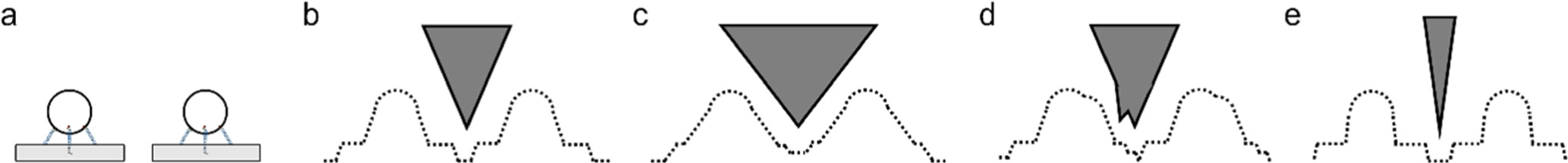
Figure 19. Schematic of different aspect ratio AFM tips interacting with samples with tall features where (a) represents the true sample.
Download figure:
Standard image High-resolution image
6.2.1. Examples of uncertainty considerations in AFM experiments
For experiments measuring the distances between functional elements, any uncertainties in the shape of the tip or events in which large molecules adhere to the tip will increase uncertainty in the measured distances, as the height trace peaks are convolutions of the shape of the functional element and the tip. AFM measurements require that the DNA structures be bound to a surface, such as mica. This binding can change structure conformation, resulting in inherent uncertainty in the use of bound state measured distances to predict those present in solution. Surface binding also quenches the structure's dynamic motion that is present in solution.
6.2.2. Examples of compatibility considerations for AFM experiments
AFM requires strong adhesion between structure and surface. This adhesion between a negatively charged mica or silica surface and negatively charged structure is normally mediated a cationic salt bridge, typically Mg2+. Designs, particularly 3D designs, with less surface area will bind the surface weakly and image poorly. Similarly, purification processes, imaging conditions, or functional elements which change surface binding can also change image quality. For example, nanostructures that were purified through gel-extraction using intercalating dyes, which are often cationic, may have a sufficiently neutralized charge to prevent surface binding.
6.2.3. Practical considerations
A rule of thumb for AFM imaging of DNA nanostructures is to keep careful track of the buffers and surface conditions, as either can prevent binding or introduce unexpected imaging artifacts. The most common surfaces for DNA nanostructures are mica substrates as they can be easily cut, glued to a puck, and cleaved or exfoliated with adhesive tape to generate a clean atomically flat surface. The typical buffering agent, trishydroxymethylaminomethane or 'tris', and the typical divalent cation, Mg2+, will precipitate together over long periods of time. Imaging with fresh buffer is a common initial troubleshooting step.
For structures with lower surface area, e.g. 3D nanostructures, the salt bridge ion can be used at higher concentrations to strengthen binding [116]. In case of particularly weak surface binding, Ni2+ can be used as it more tightly binds the DNA molecule to the mica substrate [117], though it is more prone to precipitation than Mg2+ [116]. Varying the concentrations of monovalent/divalent ions in the imaging solution can be used to control the adhesion and surface diffusion of the nanostructures [118, 119].
Circumstances in which AFM might be a poor choice include those in which high resolution is required, those in which high aspect ratio functional elements are used, those in which strong surface binding is unlikely, as well as most circumstances with a 3D structure.
6.3. Electron microscopy
Transmission electron microscopy (TEM) is another widely used verification technique for DNA nanostructures. EM works similarly to optical microscopy, except that electrons are used instead of photons. Electrons have a much smaller wavelength compared to photons, allowing for a smaller diffraction limit, but typically must travel in vacuum. Any general rules for classes of techniques as broad as AFM and EM will be full of exceptions. However for the equipment available to a typical lab, EM methods will often provide images of larger areas, often at higher lateral resolution, but will require more sample preparation.
Low atomic number elements such as those in DNA interact weakly with electrons, resulting in poor contrast relative to an underlying support grid, often made of carbon. Chemical stains using salts containing a high atomic number element are used to enhance contrast and may be necessary for imaging in some cases. High contrast functional elements, e.g. metallic or semiconducting nanoparticles, often obviate contrast concerns entirely, especially when the distance between them is the figure of merit.
Another mitigation strategy for the low contrast of biomolecules is class averaging. In brief, images containing structures are taken, then images of individual structures are binned into classes, usually based on rotation and alignment of some model 2D or 3D structure. Finally, all the aligned structures in each class are averaged to create idealized examples, even allowing for 3D reconstructions. Class averaging can create beautiful and highly precise images, but by its nature abstracts variation within a class. This is a powerful tool if most of the variation comes from imaging artifacts, such as variation in stain depth, but is potentially problematic if the variation within the imaged structures comes from a relevant structural feature, e.g. damage, missing staples, or structure motion.
6.3.1. Examples of uncertainty considerations in TEM experiments
The magnification of electron microscopes must be regularly calibrated; lack of recent calibration can result in measurement differences between labs. Both staining protocols and surface binding to TEM grids can change the conformation of a structure relative to solution [120, 121], resulting in inherent uncertainty in the use of TEM measured distances to predict solution behavior.
6.3.2. Examples of compatibility considerations for TEM experiments
TEM has a positive compatibility with functional elements that absorb or scatter electrons, e.g. metallic or semiconducting nanoparticles, as these provide contrast. TEM is also typically considered to be more compatible with 3D nanostructures than 2D nanostructures, as the former tend to be denser and thus provide better contrast during staining.
6.3.3. Practical considerations
Often, TEM is employed when the functional elements themselves have high density or elemental composition that interacts with electrons, increasing contrast, as with metallic or semiconducting particles. This can directly reveal detailed information on the assembly, shape, and positioning of the decoration element [122, 123]. Metal NPs provide very high contrast [124].
For typical DNA nanostructure experiments and equipment, TEM requires slightly more complex sample preparation which incurs an initial time cost. Once sample preparation and imaging conditions are optimized, it enables rapid imaging of large numbers of particles within short time.
6.4. Cryo-electron microscopy
Cryo-electron microscopy, Cryo-EM, is a variant of TEM in which the sample is cryo-fixed in vitreous ice, rather than dried and immobilized to a surface. Because the sample is frozen in its solvated state, the spatial relationships between molecular components are kept close to those of the solution state [125]. Cryo-EM is also often used when lower low doses are needed to avoid damage to the molecules. This is true for tomography where images are taken at multiple angles for the same structure to enable a 3D reconstruction. Each image must be acquired at a low dose to keep the cumulative dose at an acceptable level. The low signal-to-noise images require sophisticated processing to reconstruct 3D images, including class averaging. This allows information from multiple molecules to be combined to improve signal-to-noise.
6.4.1. Examples of uncertainty considerations in Cryo-EM experiments
The uncertainty considerations for Cryo-EM are similar to TEM, including those associated with class averaging.
6.4.2. Examples of compatibility considerations for Cryo-EM experiments
The compatibilities for Cryo-EM are similar to TEM, except in that Cryo-EM typically has additional time overhead for sample preparation and analysis. This can be mitigated with automated sample preparation and imaging equipment.
6.4.3. Practical considerations
This technique provides a 3D, high spatial resolution macromolecular reconstruction which could not be created otherwise [126]. However, the complex image post-processing for 3D reconstructions is non-trivial. Further optimizations map pseudo-atomic models to the Cryo-EM tomography images and allow for detailed reconstruction of DNA molecules [126, 127].
6.5. Optical super resolution microscopy
The super resolution microscopy (SRM) class of techniques exchanges resolution in time for additional resolution in space using statistical inference. This is to say, rather than imaging a structure with fluorescent molecules, photon counts are acquired across the imaging space and statistical models for the diffraction of photons are fit to these counts. This allows localization of the emitters at a resolution below that set by diffraction [128–130].
The model for the diffraction of photons from a single molecule emitter is called a Point Spread Function, or PSF [129, 130]. Typically, fluorophores switching between ON and OFF fluorescent states, or blinking, ensures that only one within a region the size of the PSF is emitting at a time. Under these circumstances, the location of an individual fluorophore may be determined with nanometer precision. Not all SRM techniques depend on the blinking behavior of the fluorophores themselves. Point Accumulation in Nanoscale Topography, PAINT, [131] achieves the same effect by means of the temporary binding of fluorescent probes diffusing in solution. The DNA-PAINT technique controls blinking through the transient hybridization of a fluorophore-labelled DNA oligomer (imager probe) with an immobilized complementary DNA strand, or docking strand [132]. The transient fluorescent signal is then captured by a fast acquisition camera and its position recorded over time acquiring a series of imaging frames. DNA-PAINT is often used in combination with a total internal reflection fluorescence, TIRF, microscope to excite imager probes close to the sample surface and reduce background fluorescence. Usually, the camera integration time is kept close to the binding time of the imager probe/docker pair to establish a high signal-to-noise ratio [133].
Since it directly targets short strand hybridization, DNA-PAINT can image the position of strands that are active in the decoration process like sticky ends or their complementary strands. It is also helpful to troubleshoot measuring the availability of sticky ends, especially if it is combined with other techniques like AFM [134].
6.5.1. Examples of uncertainty considerations in DNA-PAINT experiments
Verification of nanostructures via DNA-PAINT uses known information about the system design and the localization positions to infer the presence or absence of specific DNA strands or functional elements. Any uncertainty in the statistical inference used to localize emitters, or uncertainty that the design of the structure reflects reality, will influence propagation of the uncertainty in the DNA-PAINT experiment.
6.5.2. Examples of compatibility considerations for DNA-PAINT experiments
Structures which exhibit dynamic motion will reduce localization precision accordingly. Steric hindrance, whether by the shape of the structure or placement of functional elements, can inhibit the diffusion of the probe strand. This also means that DNA-PAINT is useful for evaluation of strand accessibility in the different areas of the structure [135, 136].
6.5.3. Practical considerations
DNA-PAINT allows acquisition of large fields of view, enabling the analysis of large numbers or structures, large arrays, or hierarchical DNA nanostructures with high precision [137]. It is an excellent choice if quantitative molecular binding measurements are needed in vitro and/or in vivo. Moreover, the probe sequence design enables multiplexing to analyze different DNA strand targets on the same DNA nanostructure surface. Although recent developments [138, 139] offer faster DNA-PAINT workflow, low imaging speed and complex image-processing remain a major drawback of this technique and limit its implementation.
6.6. Spectroscopy
Spectroscopy, particularly fluorescent or ultraviolet-visible spectroscopy, UV-Vis, can be used for bulk verification. In both, one typically infers a concentration, or similar quantity, through a modeled extinction coefficient or fluorescence efficiency. UV-Vis can also provide information on hybridization as the hyperchromicity of DNA means that ssDNA can absorb as much as 40% more than dsDNA. UV-Vis concentration data is typically measured at the 260 nm wavelength, and protein contamination is usually estimated via the ratio of absorption at 260 nm and 280 nm. There are sequence dependent models for UV-Vis extinction coefficients [140, 141], though the accuracy of these for large fully assembled structures has not been tested.
Circular dichroism, CD, uses the same wavelengths as UV-Vis but reports the difference in absorption between left-polarized and right-polarized light. It provides information on a sample's chirality and can more clearly differentiate between coiled ssDNA and helical dsDNA than absorbance hyperchromicity. Förster resonance energy transfer, FRET, is one of the most common spectroscopy techniques for DNA nanostructures and DNA origami [142]. It relies on the separation-dependent (typically sixth power as a function of distance) energy transfer between a donor and an acceptor dye molecule. The characteristic distances for FRET are typically 5 nm to 10 nm. For this reason it is used to detect distance changes, often between parts of DNA nanostructures, e.g. to detect actuation when DNA nanocontainer or nanocages are being analyzed [143–145]. Fluorophores can be easily linked to specific locations of the structure via labelled DNA strands and their signal acquired with a fluorescence microscope. This has also been used for real-time monitoring of assembly [146] and conformational folding [147].
FRET pairs offer a reliable verification tool with relatively non-invasive structure modifications and are particularly well suited to structures whose function is optical signaling such as FRET beacons [148], sensors [149] and rulers [150]. However, measuring absolute concentrations with FRET requires knowledge of the fluorescence efficiency in multiple states, which makes absolute quantification uncertain. Most typically it is used to extract the relative fraction of pairs in the signaling state.
6.6.1. Examples of uncertainty considerations in spectroscopy experiments
A major source of difficult-to-quantify uncertainty in spectroscopy techniques is the validity of assumptions used in modeling the extinction coefficient, dichroism, or fluorophore quantum yield. A related source of uncertainty is polydispersity in those properties, as spectroscopy measurements are typically made in bulk.
6.6.2. Examples of compatibility considerations for spectroscopy experiments
Compatibility in spectroscopy often stems from variation in the part of the system that provides signal, whether that is the structure itself or some functional element.
6.6.3. Practical considerations
As almost all spectroscopy equipment available to the typical lab will measure the sample as a bulk ensemble, it is typically both faster and more difficult to interpret than imaging techniques or mobility-based assays. For complex systems, it is used in tandem with other techniques to provide a check on the modeling assumptions used to interpret the spectroscopy results.
7. Conclusions
DNA nanotechnology is still a young field whose manufacturing best practices and design-property relationships are still under development. The wide variety of functional elements and chemical moieties used to label those functional elements with DNA make this both a uniquely flexible manufacturing platform, and one for which the development of best practices is challenging and highly application- specific. We hope to have provided a foundation that enables practitioners to rapidly develop and evaluate protocols and so advance the state of the art.
The breadth of knowledge required to see any one DNA nanostructure application through to fruition will likely be greater than any one expert can reasonably maintain. It is therefore important that our community not only expands the toolbox of available techniques but also begins to organize it to facilitate collaborative systems engineering. In this manuscript we have attempted to collate as much of the relevant knowledge as possible, as well as to present a workflow framework to simplify decision making for new projects.
Data availability statement
No new data were created or analyzed in this study.