
Collective effects
Published June 2018
•
Copyright © 2018 Morgan & Claypool Publishers
Pages 5-1 to 5-23
You need an eReader or compatible software to experience the benefits of the ePub3 file format.
Download complete PDF book, the ePub book or the Kindle book

Permissions
Abstract
Particles in a storage ring interact with each other, as well as with the main components designed to control the beam. Although the interactions between particles are always electromagnetic in origin, they can be manifest in a variety of ways. Consequences of collective effects include loss of particles from the beam, changes in the size and shape of bunches of particles, and beam instabilities. The origins and effects of interactions between particles in a storage ring are discussed, together with some of the ways in which undesirable effects may be mitigated.
Particles within a beam in a storage ring can interact with each other in various ways. For example, a bunch of charged particles can generate electromagnetic fields, known as wake fields, within a section of the vacuum chamber; these fields can persist for some time after the bunch has passed by, and can exert forces on following bunches. Also, particles within a bunch can 'collide' as they perform betatron and synchrotron oscillations while moving around the ring. Particles within a beam can further interact through the build-up of charged particles in the vacuum chamber, created by ionisation of residual gas or dust particles; these charged particles can exert forces on particles in the beam, affecting their dynamics. Although varied in nature, these effects have the common property that their impact depends on the amount of current in the beam.
Generally, phenomena associated with the interactions between particles in an accelerator are known as collective effects, and are manifest in various ways. In an electron storage ring, the impact of a particular kind of interaction may be limited to some change in the equilibrium distribution of particles within a bunch; for example, the emittance or energy spread may be observed to increase with the total charge of the bunch. Some collective effects may have a more significant impact, in preventing a bunch from reaching an equilibrium distribution. In such cases, the collective effect is known as a beam instability. Ultimately, collective effects may lead to the loss of particles from the beam, with a significant drop in beam current occurring on timescales ranging from several hours to a fraction of a second, depending on the loss mechanism. Modern storage rings often require high beam currents to achieve their performance specifications. Understanding and (where possible) mitigating collective effects is then an essential part of the design and operation of the storage ring. In this chapter, we shall consider some of the principal collective effects commonly encountered in electron storage rings. These include scattering effects (from collisions between particles) leading to limitations on the beam lifetime, and the effects of wake fields that often result in beam instabilities.
5.1. Touschek scattering and space charge
We begin by considering the scattering processes that occur when two particles within a bunch collide. One effect of this scattering, as we shall see, is the loss of particles from the beam. The limit that this imposes on the beam lifetime is an important aspect of the operational performance of many modern electron storage rings.
As a bunch of particles moves around a storage ring, particles within the bunch perform betatron and synchrotron oscillations. Occasionally, in the course of these oscillations, two particles may come close enough to each other that the force between them is sufficiently large to cause a significant change in their motion. In the case of electrons, such an interaction is described by Møller scattering [1]. The theory of Møller scattering gives the differential cross-section that describes the probability for two electrons to be deflected by a certain angle following a collision. Suppose, for example, that two electrons move towards each other along trajectories that are parallel to the x (horizontal, transverse) axis, but with some small separation. As they move past each other, the electrons can be deflected so that there is some vertical and longitudinal component to their motion. If the deflection angle is fairly small, the only consequence may be some transfer of momentum between the different degrees of freedom of the particle motion. This may be observed in a storage ring as a change in the beam emittances, in a process known as intrabeam scattering (IBS) [2, 3]. Although IBS takes place continually in bunches consisting of large numbers of particles, the rate of change of the emittances that happens as a result of IBS in an electron storage ring is usually slow compared to the synchrotron radiation damping times. This means that the effects of IBS in electron rings are generally difficult to observe, and only become significant under special conditions of high particle density [4–6]. If the particle density is increased by increasing the number of particles in a bunch, then other collective effects can start to impact the dynamics, masking the effects of IBS; usually the best way to observe IBS in an electron storage ring is to reduce the vertical emittance to as low a value as possible.
A more important effect occurs when two particles in a bunch approach each other closely enough that they are deflected through an angle leading to a significant transfer of momentum from a transverse to the longitudinal direction. Since the betatron tunes are generally much larger than the synchrotron tune, in the rest frame of the bunch the transverse component of the momentum will be larger than the longitudinal component, for most of the particles in the bunch. This means that scattering between particles can lead to a significant increase in the longitudinal momentum of the particles; it is then possible that following a scattering event, the energy deviation of one or both of the particles involved will be outside the energy acceptance of the storage ring (as discussed in section 4.4). In that case, the particles will be lost from the beam, and the process is known as Touschek scattering [7]. The observable effect is that the beam current in the storage ring decays over time. The rate of decay depends on the beam energy, the beam size (transverse and longitudinal) and the bunch population. In a parameter regime typical for a third-generation synchrotron light source, the Touschek lifetime characterising the decay rate is usually a number of hours. Other processes (for example, the scattering of electrons from residual gas molecules in the vacuum chamber) also lead to the loss of particles from the beam, but at low emittance and high bunch charge, Touschek scattering normally dominates the beam lifetime.
The rate of loss of particles from a beam by Touschek scattering is proportional to the square of the number of particles in a bunch; strictly speaking, this means that the beam current does not decay exponentially. However, for a short time interval (over which the bunch population is roughly constant) the fall in current can be approximated as an exponential decay, so that

where I(0) is the initial beam current, I(t) is the beam current at time t. The Touschek lifetime τT is given by

where
Nb is the bunch population, re
is the classical radius of the electron
1
, γ is the relativistic factor for particles in the bunch,
σx
,
σy
, and
σz
are the horizontal, vertical, and
longitudinal rms beam sizes,
 is the energy acceptance of the ring, and
D(ξ) is the function
is the energy acceptance of the ring, and
D(ξ) is the function

The parameter ξ is defined by

where βx is the horizontal Courant–Snyder parameter, and εx is the horizontal emittance. The Touschek function D(ξ) is plotted in figure 5.1.
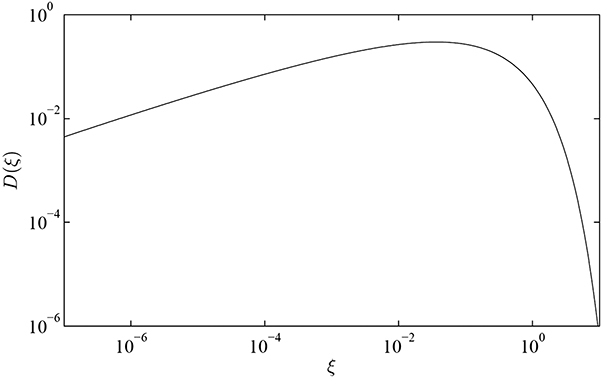
Figure 5.1. The Touschek function D(ξ), defined by equation (5.3). The parameter ξ (5.4) increases with the energy acceptance of the storage ring, and decreases with the beam energy and the emittance. The Touschek lifetime is proportional to the third power of D(ξ).
Download figure:
Standard image High-resolution imageParticles in a beam in an accelerator can be affected not just by individual scattering events, but also by interaction with the electromagnetic field generated collectively by all the particles in a bunch. If we consider a bunch of electrons at rest in the laboratory, the electrostatic repulsion between the electrons will cause the bunch to expand rapidly—the bunch will not survive very long. In an accelerator, relativistic effects act in two ways to reduce the rate of expansion of a bunch travelling at close to the speed of light. First, Lorentz contraction means that a bunch that appears relatively short (of order of a few millimetres) when moving in an accelerator will be longer by the relativistic factor γ in the rest frame of the bunch, with the result that the charge density will be reduced by the same factor. Second, time dilation means that the expansion rate of the bunch in the accelerator is reduced by a factor γ when observed from the laboratory rest frame. Overall, the expansion rate is reduced by a factor γ2 compared to a bunch with the same dimensions observed in its rest frame. For a beam at 2 GeV in an electron storage ring, γ is roughly 4000, so the suppression of the effects of the Coulomb repulsion by a factor γ2 is significant.
Another way of looking at the (effective) suppression of the Coulomb repulsion is by considering the fields around a bunch of particles moving through an accelerator. The moving charged particles constitute an electric current, which generates a magnetic field around the bunch. A particle within the bunch sees both the electric field and the magnetic field. Although the force from the electric field acts to push the particle out of the bunch, the force from the magnetic field is such as to pull the particle towards the bunch. A detailed analysis shows that overall, the transverse acceleration of a particle resulting from the combined electric and magnetic fields is reduced by a factor γ2 in comparison to the acceleration that would be expected for a bunch of particles at rest (with no magnetic field). This is consistent with the same result obtained by considering the effects of time dilation and Lorentz contraction.
Although the Coulomb repulsion is suppressed in an accelerator, the fact that the relativistic factor γ is always a finite quantity means that there are always some residual effects from this repulsion, these are generally known as space charge effects. In the transverse directions, space charge forces may be viewed as defocusing forces, since the size of the force varies with distance from the centre of the bunch: space charge forces can then affect the tunes and the Courant–Snyder parameters in a storage ring. However, because of the way in which charge is usually distributed within a bunch, the defocusing force is strongly nonlinear, and different particles will experience different defocusing strengths depending on their transverse and longitudinal position within the bunch. Space charge then leads to a spread of different tune values for different particles, sometimes called an incoherent tune shift. However, since the relativistic factor is typically quite large in electron storage rings, space charge effects are usually weak, and although they may be significant in certain parameter regimes, we do not consider space charge effects further here. Further discussion can be found in, for example, [8–11].
5.2. Ion trapping
Storage rings must achieve extremely low residual gas pressures within the beam pipe (or vacuum chamber) for two main reasons. First, particles in the beam can scatter from gas molecules in the beam pipe and be lost from the beam as a result—this can limit the beam lifetime. Second, gas molecules can be ionised by the electromagnetic fields around the beam, and the ions produced in this way can interact with the beam, potentially causing it to become unstable. Pressures of order of 1 nTorr are routinely achieved in electron storage rings; for comparison, atmospheric pressure is roughly 760 Torr.
Ion effects [12, 13] can be particularly damaging in a storage ring if the ions build up to high densities. The forces exerted by the ions can deflect the trajectories of bunches in the beam; the beam in turn deflects the ions, and it is possible for a cycle to develop in which the beam starts to perform oscillations of increasing amplitude, leading eventually to the loss of beam current. Beam loss is most likely to occur if ions become trapped in the beam, reaching high densities as ions continue to be generated from the residual gas molecules in the vacuum chamber. Ion trapping can be understood in terms of the focusing effects of the fields around bunches in the beam—the electric and magnetic fields generated by a bunch leads to forces on the ions that increase with transverse distance from the centre of the bunch. In that respect, the forces are similar to those from quadrupole magnets acting on particles in the beam; however, the forces experienced by ions from the fields around the beam are focusing both horizontally and vertically, and are also strongly nonlinear. Despite the nonlinear nature of the forces, it is possible to analyse the dynamics of ions in the beam in much the same way as the dynamics of particles in the beam can be analysed as the beam moves through (for example) a FODO beam line. In both cases, particles receive regular 'kicks' separated by drift lengths.
In the case of particles travelling along a FODO beam line, there are constraints on the quadrupole strengths and separations for the particle motion to be stable. There are corresponding constraints on the focusing forces experienced by ions and the bunch separation for the motion of the ions to be stable in the presence of a beam. The stability condition can be expressed in terms of the mass to charge ratio A/Q of the ions (with A the relative atomic mass, and Q the charge of the ion in units of the elementary charge e). Ions can be trapped (perform stable oscillations) in the beam if [13]

where Nb is the number of particles in each bunch in the beam, bunches have regular separation Lsep, rp is the classical radius of the proton, and σx and σy are the horizontal and vertical rms beam sizes, respectively. It is assumed that σy < σx , which is usually the case in an electron storage ring.
In many cases, it is inevitable that some species of ion generated from residual gas molecules in the vacuum chamber will be trapped in the beam. Unfortunately, improving the gas pressure cannot help, since gas molecules cannot be entirely removed from the chamber, and the ion density will eventually build up to sufficiently high levels as to cause beam instability. An effective mitigation, however, is to include a gap in the bunch train, of sufficient length to disrupt the focusing effect of the beam and destabilise the motion of the ions. Although this means that some beam current must be sacrificed because a number of the RF buckets will be empty, the benefit in terms of beam stability is usually essential for meeting the performance required of the storage ring.
5.3. Wake fields, wake functions, and impedances
The electromagnetic fields generated by charged particles in the beam in an accelerator are modified by the presence of the vacuum chamber and components such as RF cavities, beam position monitors, flanges (where sections of beam pipe are joined together), and bellows (that allow for some expansion or movement of the beam pipe). As particles pass a given section of beam pipe, they can excite oscillating electromagnetic fields in that section that may persist for some time after the bunch has passed by. These fields, known as wake fields, can exert forces that affect the motion of other particles within the accelerator [14, 15]. Wake fields are sometimes categorised as short range or long range. Short range wake fields are those that are generated and act back on particles within a single bunch. In an electron storage ring, bunch lengths are typically a few millimetres. Long range wake fields persist for much longer, and act on bunches following the bunch originally generating the wake field; the length scale in this case can be anything from around a metre, to some hundreds of metres. An example of the wake fields in a section of accelerator beam pipe generated by an electron bunch is shown in figure 5.2.
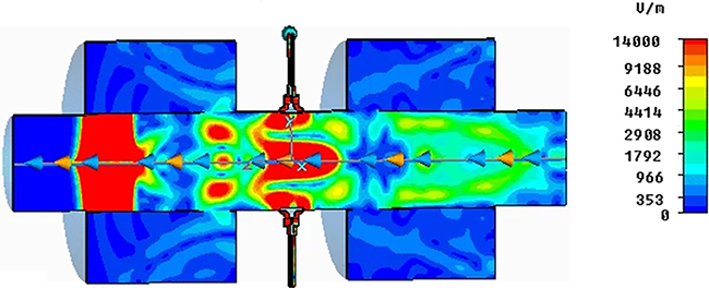
Figure 5.2. Wake fields in a section of accelerator beam pipe containing a beam position monitor (BPM). A cross-section (in the vertical–longitudinal plane) of the beam pipe is shown, with the beam moving from right to left. The colours show the strength of the electric field generated by a bunch of electrons: the bunch is located in the large red area (high electric field strength) towards the left of the diagram. The pick-up electrodes for the BPM are in the centre of the section of beam pipe, with bellows (to allow some flexibility in the beam pipe position on either side of the BPM) on the left and right of the electrodes. Copper strips (not visible in the diagram) are positioned to prevent the electric fields penetrating into the bellows.
Download figure:
Standard image High-resolution imageCalculating the wake fields as functions of position and time from a bunch with given dimensions and charge, and in a section of beam pipe with given geometry and materials, is a complex computational problem, usually involving numerical solution of Maxwell's equations [16, 17]. The task can be computationally expensive, because of the range of distance scales involved. The bunch generating the wake fields may be a few millimetres long, but much less than a millimetre in width and height. This implies the need to model the fields on a grid (in space and time) with a spacing between grid points of a fraction of a millimetre. However, the grid may need to cover a volume with dimensions of several centimetres transversely and up to a metre longitudinally. Assuming that the wake field in a given situation can be computed, determining its impact on the beam in an accelerator is another formidable challenge. There is again a very wide range of distance and time scales involved, and it is usually not feasible to compute the motion of each individual particle even within a single bunch, which may contain of order 1010 particles.
There are also numerous ways in which wake fields may affect beam behaviour. In some cases, there may simply be some increase in the transverse or longitudinal dimensions of a bunch, but with the shape of the bunch (usually, in an electron storage ring, described by a Gaussian distribution function) remaining the same; or, the shape of the bunch may change as it moves around the ring. An example of the impact of wake fields on the longitudinal phase space charge density in a single bunch in a storage ring is shown in figure 5.3. As well as changing the charge distribution with a bunch, wake fields can change the betatron or synchrotron tunes, in which case the effects can depend on the proximity of the nominal tunes to resonances. Entire bunches may start to oscillate, either transversely or longitudinally. Finally, the problem is further complicated by the fact that as the beam responds in some way to the presence of wake fields, the wake fields that it continues to generate will change, because of changes in the size, shape or trajectory of the bunches. For an accurate description of beam behaviour in a storage ring with wake fields, it may be necessary to find a self-consistent solution to the full system including the generation of the wake fields and the dynamics of the beam in the presence of the wake fields.
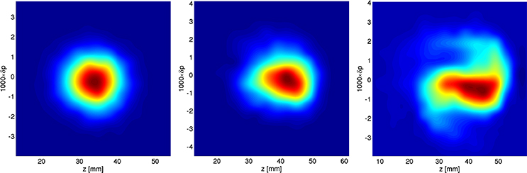
Figure 5.3. Simulation of the effect of wake fields on the charge distribution in longitudinal phase space of a single bunch in a storage ring. At low charge (left-hand image) the bunch distribution is Gaussian, and stable. At higher charge (middle image) some distortion is visible on the distribution. If the bunch charge is increased still further (right-hand image) the distortion becomes more pronounced. In this case, the distribution fails to reach an equilibrium, but continuously changes shape.
Download figure:
Standard image High-resolution imageGiven the complexity of the problem, it is not surprising that we look for simplified models that can nevertheless give us some insight into the beam behaviour, and have some value not only in predicting how a beam will be affected by wake fields in a given accelerator design, but also how the design may be optimised in order to achieve the best possible performance. The first simplification is to represent the wake fields by wake functions [14], which describe the change in energy or momentum of one particle as it follows another particle through a given section of the accelerator beam line. In particular, we can define a longitudinal wake function W∥( −Δz) with units of V C−1 (volts per coulomb), such that

where the wake field is
generated by a particle (or small bunch of particles) with charge
qA and longitudinal co-ordinate
zA, and a trailing particle with charge
qB and longitudinal co-ordinate
zB undergoes a change in energy deviation
ΔδB over the length of the given accelerator section.
E0 is the reference energy and
 . Note that Δz is positive
for
. Note that Δz is positive
for
 , i.e. if particle A is ahead of particle
B—causality implies that
, i.e. if particle A is ahead of particle
B—causality implies that
 if Δz is negative.
Similarly, we can define a transverse wake function
 with units of V C−1
m−1, which gives the transverse deflection of particle B as it follows
particle A through a given section of the accelerator:
with units of V C−1
m−1, which gives the transverse deflection of particle B as it follows
particle A through a given section of the accelerator:

Here, py, B is the vertical momentum of particle B scaled by the reference momentum, and yA is the vertical co-ordinate of particle A. This formula assumes that the transverse deflection of particle B has a linear dependence on the transverse position of particle A. This may be a good approximation over a small range of transverse offsets from the reference trajectory (which we assume coincides with the centre of the beam pipe), but will break down at some point.
There are two main benefits of working with wake functions rather than wake fields. First, the wake field depends on the properties (charge, size and shape, trajectory) of the bunch generating the wake field as well as on the properties (geometry, materials) of the section of beam pipe under consideration. Using a wake function allows us to separate the properties of the bunch generating the wake fields from the properties of the beam pipe—a wake function describes a section of the accelerator, regardless of the beam passing along the accelerator. The second benefit is that wake functions reduce a wake field that is a complex function of position (in three dimensions) and time, to a relatively simple function that depends only on one variable, namely the longitudinal separation between a point-like particle generating a wake field, and a point-like particle observing the wake field. Both benefits, of course, come at the sacrifice of some accuracy and completeness in the description of the system. In many cases, however, the use of wake functions rather than wake fields makes it possible to gain some insight into the behaviour of a system (a beam in an accelerator) that would otherwise be hopelessly complicated.
In some cases, wake functions can be calculated analytically by finding a solution to Maxwell's equations for the fields around a point charge moving close to the speed of light, with the boundary conditions imposed by the vacuum chamber [14, 18]. For example, in the case of a long, straight vacuum chamber of length L and with uniform circular cross-section of radius r, the longitudinal wake function is given (for Δz > 0) by

where Z0 is the impedance of free space, and σ is the conductivity of the vacuum chamber material. The transverse wake function is given (again for Δz > 0) by

Since the wake fields in this case arise essentially from the finite conductivity of the vacuum chamber, these wake functions are known as the resistive wall wake functions. By causality, both wake functions vanish if the particle observing the wake fields is ahead of the particle generating the wake fields, i.e. if Δz < 0. It should also be noted that the above expressions involve approximations that are valid if

Although analytical calculations are possible in some cases, wake functions generally need to be computed the same way as wake fields, by solving Maxwell's equations numerically in a given section of beam line; unfortunately, the computation of a wake function can be more difficult than that of a wake field, since the source of the fields should ideally be represented as a point-like particle. This raises certain computational difficulties, which we do not discuss further. For an overview of methods used for computing wake functions, see (for example) [17] and references therein.
Wake functions provide a description of wake fields in the time domain. A wake function is a function of the longitudinal separation of two particles (where the longitudinal separation is specified in terms of the co-ordinate z which, it should be remembered, actually gives the time that a particle arrives at a given point in the beam line). It turns out that in many cases, the most damaging wake fields are associated with resonances in the beam pipe, where fields oscillating at some specific frequency (the resonant frequency) can persist for long periods of time. In such cases, it is often more convenient to work with a description of the wake fields in the frequency domain, in which case we express the wake function as a superposition of sinusoidal functions of different frequencies. In other words, we work with the Fourier transform of the wake function, which is known as the impedance [14, 15, 19]. The longitudinal impedance is defined by

and the transverse impedance is defined by

With these definitions, the longitudinal wake function can be expressed in terms of the longitudinal impedance by an inverse Fourier transform:

Similarly, for the transverse wake function

Note that the
longitudinal impedance has units of Ω (ohms), while the transverse impedance has units
of
 (ohms per metre).
Simply knowing the form of an impedance for a section of accelerator beam line can be useful in providing some indication of whether the wake fields are likely to have a strong impact on the beam. This is because the effect of the wake field depends on the convolution of the beam spectrum (i.e. the frequencies present in the beam current observed at a particular location as a function of time) and the impedance. In particular, it can be shown (see, for example [10]) that

where
 is the Fourier spectrum of the voltage (seen
by a particle in the beam) across a section of beam line with impedance
is the Fourier spectrum of the voltage (seen
by a particle in the beam) across a section of beam line with impedance
 , and
, and
 is the beam current spectrum. If the beam
current has a component at a frequency where the impedance is large (perhaps associated
with a resonance), then there will be a large voltage induced across that section of the
beam line, leading to a large change in energy of the particles in the beam as they pass
through. This could have a significant impact on the beam behaviour, potentially leading
to an instability. On the other hand, if the impedance is small at the frequencies that
dominate the beam current spectrum, the wake fields are unlikely to have any great
impact on the beam. The above equation (5.15) is, of course, just the usual
relationship between voltage, current, and impedance, applied to the beam in an
accelerator.
is the beam current spectrum. If the beam
current has a component at a frequency where the impedance is large (perhaps associated
with a resonance), then there will be a large voltage induced across that section of the
beam line, leading to a large change in energy of the particles in the beam as they pass
through. This could have a significant impact on the beam behaviour, potentially leading
to an instability. On the other hand, if the impedance is small at the frequencies that
dominate the beam current spectrum, the wake fields are unlikely to have any great
impact on the beam. The above equation (5.15) is, of course, just the usual
relationship between voltage, current, and impedance, applied to the beam in an
accelerator.
5.4. Potential-well distortion
In an electron storage ring, a common observation is that the longitudinal profile of a bunch (i.e. the charge per unit length, as a function of position along the bunch) depends on the amount of charge in the bunch (see, for example [20, 21]). In section 3.2.3 we saw that synchrotron radiation effects lead to an equilibrium rms bunch length σz given by (3.40)

where
 is the phase slip factor of the lattice
(2.77),
ωs is the synchrotron frequency (2.80), and
σδ
is the rms energy spread (3.39). This
expression gives the bunch length that we expect in the limit of low bunch charge, but
as the bunch charge increases the wake fields that are generated by a bunch lead to an
increase in the bunch length. This effect is known as potential-well
distortion [14]. Usually, potential-well distortion does not have a severe impact on the
operation of an electron storage ring, but it can be an interesting effect to study
since the behaviour of the bunch can provide some information about the wake fields in a
storage ring. If the bunch charge is increased sufficiently, then rather than merely
increasing in length, the bunch can become unstable, and this can have an adverse impact
on machine performance. Understanding the wake fields is therefore an important aspect
of the design and operation of a storage ring.
is the phase slip factor of the lattice
(2.77),
ωs is the synchrotron frequency (2.80), and
σδ
is the rms energy spread (3.39). This
expression gives the bunch length that we expect in the limit of low bunch charge, but
as the bunch charge increases the wake fields that are generated by a bunch lead to an
increase in the bunch length. This effect is known as potential-well
distortion [14]. Usually, potential-well distortion does not have a severe impact on the
operation of an electron storage ring, but it can be an interesting effect to study
since the behaviour of the bunch can provide some information about the wake fields in a
storage ring. If the bunch charge is increased sufficiently, then rather than merely
increasing in length, the bunch can become unstable, and this can have an adverse impact
on machine performance. Understanding the wake fields is therefore an important aspect
of the design and operation of a storage ring.
To estimate the impact of wake fields on the longitudinal dynamics of particles in a storage ring, we can perform an analysis based on the same equations of motion that we used previously (in section 3.2.1), but including an additional term to represent the change in the energy deviation from the effects of wake fields. The equations of motion for the longitudinal co-ordinate z of a particle and the energy deviation δ can be written in the form


Here,
αp
is the momentum compaction factor
(2.72),
E0 is the reference energy, C0
is the circumference of the storage ring, and
 is the charge per unit length of the bunch,
as a function of longitudinal position
is the charge per unit length of the bunch,
as a function of longitudinal position
 in the bunch. The wake function
 represents the longitudinal wake fields over
the entire circumference of the ring. The integral arises from summing the wake fields
generated by all particles in the bunch that are ahead of the particle for which the
equations of motion are written.
represents the longitudinal wake fields over
the entire circumference of the ring. The integral arises from summing the wake fields
generated by all particles in the bunch that are ahead of the particle for which the
equations of motion are written.
Solving the equations of motion (5.17) and (5.18) is not an easy task; however, we are interested in finding the equilibrium longitudinal distribution, rather than a full solution to the equations of motion. A way of finding the equilibrium longitudinal distribution is provided by the observation that the equations of motion have a conserved quantity 2 :

Since the equilibrium distribution, by definition, remains the same as the bunch moves around the storage ring, it should be possible to express the equilibrium charge distribution as a function of a conserved quantity. Assuming that the charge distribution within a bunch in an electron storage ring is (at low bunch charge) Gaussian, we write the equilibrium distribution Ψ(z, δ) (the charge per unit area of longitudinal phase space) as

where Ψ0 is a constant, chosen so that integrating the charge density Ψ(z, δ) over all values of z and δ gives the total charge in the bunch. If we integrate the equation above for Ψ(z, δ) just over the energy deviation δ, we obtain

where λ(z) is the charge per unit length in the bunch,

and the constant
λ0 is chosen so that the integral of the charge per unit
length over the entire length of the bunch gives the total charge in the bunch. Equation
(5.21) is known
as the Haissinski equation [22]—it is an integral equation for the
equilibrium longitudinal charge distribution λ(z). If
all other quantities are known (including the longitudinal wake function
 ), then it is possible to solve the Haissinski
equation to find the longitudinal distribution λ(z).
Usually, the solution has to be found numerically.
), then it is possible to solve the Haissinski
equation to find the longitudinal distribution λ(z).
Usually, the solution has to be found numerically.
Despite the approximations made in describing the wake fields by means of a wake function, it is often found that (given an appropriate model for the wake function) the Haissinski equation provides a good description of the longitudinal profile of a bunch as a function of the bunch charge in a storage ring. In particular, the Haissinski equation describes the increase in the rms bunch length with increasing bunch charge (see figure 5.4). In physical terms, the wake fields cause a loss of energy of particles in a bunch, and this energy has to be replaced by the RF cavities. As the energy loss increases with increasing bunch charge, the synchronous phase moves closer to the peak of the RF voltage, where the gradient of the RF (rate of change of voltage with time) is smaller. Since the gradient of the RF provides the longitudinal focusing in a storage ring, a smaller slope means less focusing, which results in a longer bunch.
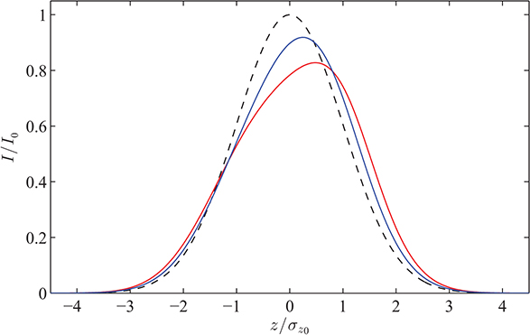
Figure 5.4. Potential-well distortion in an electron storage ring. The horizontal axis indicates the longitudinal position with respect to the reference particle, and the vertical axis indicates the beam current (corresponding to the number of particles per unit length as a function of position along the bunch). At low bunch charge, the bunch has a Gaussian longitudinal profile (dashed black line). At higher bunch charge, wake fields lead to potential-well distortion, resulting in a longitudinal profile that is no longer Gaussian (solid blue line). If the ring is above transition, then the width of the bunch is increased, and the distribution 'tilts' forward. If the bunch charge is increased (solid red line) then the tilt becomes more pronounced.
Download figure:
Standard image High-resolution image5.5. Microwave instability
Potential-well distortion in an electron storage ring leads to an increase in bunch length, but the energy spread is not significantly changed—as long as the wake fields are not too strong, the energy spread remains close to the value (3.39) expected from the balance between synchrotron radiation damping and quantum excitation. However, if the bunch charge is increased sufficiently, then it is found that above some threshold bunch charge, the energy spread starts to increase as well as the bunch length. This can be explained in terms of an instability, known as the microwave instability [23], that is driven by wake fields. In this section, we shall derive an approximate formula for the threshold current at which we expect to see the instability occur.
By their very nature, beam instabilities are phenomena in which the charge distribution continuously evolves in time, without reaching equilibrium. In principle, instabilities may be described by considering the equations of motion of the individual particles within a bunch (or within an entire beam in a storage ring); however, since the number of particles can be very large, this is rarely a practical approach. Instead, we represent a bunch of particles not as a collection of point-like charges, but as a smooth, continuous distribution of electric charge. We can then write an equation that describes how the charge density evolves as a function of time. If we assume that we can neglect dissipative forces (in other words, we assume that the forces acting on the distribution can be derived from suitable potentials) then the appropriate equation is the Vlasov equation:

where Ψ(θ, δ; t) is the charge density as a function of the co-ordinate θ (the angular position around the storage ring) and energy deviation δ, at time t. In the case of an electron storage ring, the Vlasov equation describes the evolution of the charge density in a bunch of particles if we neglect synchrotron radiation.
To apply the Vlasov equation to find the evolution of a charge density distribution, we write for the rate of change of the co-ordinate θ

where
T0 is the revolution period for a particle with
δ = 0, and
 is the phase slip factor. We also need an
explicit expression for the rate of change of the energy deviation. To simplify the
analysis, we include only the effects of wake fields, i.e. we neglect the RF cavities
and synchrotron radiation. This means that we ignore the synchrotron oscillations of
particles in the beam, but if we apply the Vlasov equation only over a time scale that
is short compared to a synchrotron period (which may be several hundred turns of the
ring) this can be a valid approach. The rate of change of the energy deviation is then
given (in terms of the longitudinal impedance
Z∥(ω) of the entire ring) by
is the phase slip factor. We also need an
explicit expression for the rate of change of the energy deviation. To simplify the
analysis, we include only the effects of wake fields, i.e. we neglect the RF cavities
and synchrotron radiation. This means that we ignore the synchrotron oscillations of
particles in the beam, but if we apply the Vlasov equation only over a time scale that
is short compared to a synchrotron period (which may be several hundred turns of the
ring) this can be a valid approach. The rate of change of the energy deviation is then
given (in terms of the longitudinal impedance
Z∥(ω) of the entire ring) by

where e
is the magnitude of the charge on a single particle (electron, or positron) in the beam,
and  is the beam current spectrum. The expressions
for the rate of change of co-ordinate θ (5.24) and energy deviation δ
(5.25) are
substituted into the Vlasov equation (5.23); the solution of the partial
differential equation that we obtain in this way gives the evolution of the phase space
density Ψ(θ, δ; t) as a function of
time t, for a given initial distribution Ψ(θ,
δ; 0).
is the beam current spectrum. The expressions
for the rate of change of co-ordinate θ (5.24) and energy deviation δ
(5.25) are
substituted into the Vlasov equation (5.23); the solution of the partial
differential equation that we obtain in this way gives the evolution of the phase space
density Ψ(θ, δ; t) as a function of
time t, for a given initial distribution Ψ(θ,
δ; 0).
In practice, solution of the Vlasov equation usually needs to be done numerically. However, we can obtain some useful results by assuming an approximate solution of the form

where
Ψ0(δ) is an assumed constant energy distribution, and ΔΨ
is the amplitude of a modulation in the density of the particles as a function of
position around the ring. Note that the modulation takes the form of a wave travelling
around the ring, with wavelength
 and angular frequency
ωn
. By substituting the assumed
solution (5.26)
into the Vlasov equation (5.23), and integrating over the energy
deviation (to eliminate the unknown amplitude ΔΨ) we obtain an integral equation for the
oscillation frequency ωn
of the density
modulation
3
:
and angular frequency
ωn
. By substituting the assumed
solution (5.26)
into the Vlasov equation (5.23), and integrating over the energy
deviation (to eliminate the unknown amplitude ΔΨ) we obtain an integral equation for the
oscillation frequency ωn
of the density
modulation
3
:

where I0 is the average beam current, and ω = dθ / dt is the angular revolution frequency of a particle with energy deviation δ. The above equation (5.27) is a dispersion relation; it relates the frequency of the wave (representing the density modulation) to its wavelength. Given the impedance of the ring Z∥(ω), the energy spread Ψ0(δ) and the beam current I0, we can solve the dispersion relation (5.27) to find the oscillation frequency ωn of the density modulation as a function of the wavelength C0 / n. If the frequency is a real number, then the modulation will simply propagate as a wave with constant amplitude. However, if the frequency is a complex number, then depending on the sign of the imaginary part, the amplitude of the modulation will either damp or grow exponentially. In the latter case, an initially small modulation can rapidly become very large, indicating an instability in the beam.
5.5.1. Microwave instability in a 'cold' beam
As an example, consider a beam with zero energy spread, i.e. with Ψ(δ) = 0 for all δ except δ = 0. Such a beam is sometimes called a 'cold' beam. The dispersion relation in this case can be solved to give

We see that in this case there will (unless the impedance is a purely imaginary number) always be a solution for the modulation frequency ωn with a positive imaginary part. Since a beam will inevitably never have a perfectly uniform distribution around a storage ring, a cold beam will always be unstable.
5.5.2. Energy spread and beam stability: Landau damping
A more realistic example is the case where the beam has a Gaussian energy spread:

In this case, it is not possible to write an analytical solution for ωn , but it can be shown that for an impedance such that Z∥(nω0)/n is approximately constant, that the beam will be stable (the modulation frequency ωn will have a negative imaginary part) if the beam current is below the instability threshold:

It is only if the current is above Ith that the beam becomes unstable. This is in contrast to a cold beam, which was unstable for any size of beam current. The reason that the energy spread can stabilise the beam is that the revolution frequency of the particles depends (through the phase slip factor ηp) on the energy deviation. Particles with different energies will move around the ring at different rates, and this tends to smooth out any modulation that appears in the particle density. The suppression of an instability in this way is known (by analogy with a similar effect in plasma physics) as Landau damping [24, 25]. However, if the current is large enough then the enhancement of the modulation amplitude by wake fields outweighs its suppression by Landau damping, and the modulation amplitude is able to grow exponentially (indicating a beam instability).
Given the numerous simplifications and approximations we have made in the analysis, we are not able to determine with any precision how a density modulation will develop in any given situation—all we can say is whether the beam is likely to be stable or unstable, and even then there can be considerable uncertainty. We also need to be careful about applying the results to an electron storage ring, since we have neglected the effects of RF cavities and synchrotron radiation. Strictly speaking, our analysis applies to the case that there is an approximately uniform distribution of charge around the ring. However, it turns out that in practice, the wavelength of the modulation in the case of an instability is often much shorter than the bunch length; one indication of this is that the instability can be accompanied by the emission of electromagnetic radiation with wavelengths of 1 mm or less, associated with a large density modulation in an individual bunch. Because of this radiation, the instability is usually called the microwave instability. Given the short wavelength of the modulation, it is often assumed that the analysis can be applied to bunched beams, rather than just to beams with approximately uniform density around the entire ring, in which case we simply substitute the peak current in the bunch for the average current in the ring. The stability condition (5.30) is then usually expressed in terms of the impedance rather than the current:

where Z0 is the impedance of free space, σz is the rms bunch length, re is the classical radius of the electron, and Nb is the number of electrons in a single bunch. The stability condition (5.31) is known as the Keil–Schnell–Boussard criterion [23, 26].
In the analysis in this section, we have considered only the longitudinal motion of the beam. Of course, wake fields can also affect the transverse motion, leading to beam instabilities with a range of characteristics. Transverse instabilities observed in electron storage rings include the head–tail instability, and the transverse mode-coupling instability. In principle, the Vlasov equation can be extended to include transverse motion as well as longitudinal motion; however, different analysis methods can also be used. For further information, the reader is referred to other texts, for example [14].
5.6. Coupled-bunch instabilities
The effects that we considered in the previous sections, potential-well distortion and the microwave instability, result from wake fields acting over the length of a single bunch in an electron storage ring, which is typically a few millimetres. We assumed that we could neglect any effects from (long-range) wake fields acting over the distance between individual bunches, which could be many centimetres or some metres. However, long-range wake fields can affect the stability of a beam in a storage ring, and in this section we shall consider how coupled-bunch instabilities develop, how they may affect machine performance, and how they may be mitigated.
We shall base our analysis on a simple model of a beam, in which each bunch is
represented as a point-like object, with total charge
 and mass
 , where e and
m are the magnitude of the charge and the mass of the electron,
respectively, and Nb
is the bunch
population. Since we ignore any internal structure in a bunch, this approach is limited
to coherent betatron and synchrotron oscillations, where the entire
bunch oscillates transversely or longitudinally as it moves around the storage ring.
Here, we shall consider only betatron oscillations; however, synchrotron oscillations
may be treated in much the same way. To simplify the model further, we shall assume that
the betatron oscillations can be characterised by an angular frequency
ωβ
that is the same at all points around
the ring. In effect, this neglects any variation in the Courant–Snyder beta function.
With these simplifications, the equation of motion for a bunch performing vertical
betatron oscillations in the absence of wake fields is
, where e and
m are the magnitude of the charge and the mass of the electron,
respectively, and Nb
is the bunch
population. Since we ignore any internal structure in a bunch, this approach is limited
to coherent betatron and synchrotron oscillations, where the entire
bunch oscillates transversely or longitudinally as it moves around the storage ring.
Here, we shall consider only betatron oscillations; however, synchrotron oscillations
may be treated in much the same way. To simplify the model further, we shall assume that
the betatron oscillations can be characterised by an angular frequency
ωβ
that is the same at all points around
the ring. In effect, this neglects any variation in the Courant–Snyder beta function.
With these simplifications, the equation of motion for a bunch performing vertical
betatron oscillations in the absence of wake fields is

where y is the vertical co-ordinate of the bunch centroid (i.e. the centre of mass of the bunch).
We can include the effects of wake fields by adding a driving term on the right-hand side of the equation of motion (5.32). To start with, let us assume that there is only a single bunch in the storage ring. At each point in the storage ring, the bunch will generate a wake field that will act back on the bunch on later turns. In terms of the wake function (5.7) that describes the change in momentum of a particle (or, in this case, an entire bunch of particles) resulting from the wake field, the equation of motion for the bunch centroid can be written

where C0 is the ring circumference, and the index k refers to the number of turns around the ring that the bunch has performed since it generated the wake field at its present point. Since the summation over k extends to infinity, there is an assumption that the bunch has been in the ring for an infinite length of time; in practice, since the wake fields will decay over time, the summation may be truncated at some finite value of k for which the wake function becomes negligible.
To include the effects of multiple bunches in the ring, we need to add another summation, to take account of the wake fields generated by each bunch. We write the centroid of the mth bunch at time t as ym (t). Then, if there are M bunches in the storage ring we can write the equation of motion for the nth bunch as
Note that we assume that
the bunches are equally spaced around the storage ring, so that the distance between the
mth and the nth bunches is
 . We also assume that all bunches have the
same population Nb. To understand the dynamics of the beam
in the presence of wake fields, we need to find a solution to the equation of motion
(5.34). We
shall assume a solution of the form
. We also assume that all bunches have the
same population Nb. To understand the dynamics of the beam
in the presence of wake fields, we need to find a solution to the equation of motion
(5.34). We
shall assume a solution of the form

where μ is an index describing different patterns of variation of the
centroid co-ordinate ym
from
bunch-to-bunch, at a given time t. For example, for μ
= 0, all bunches have the same centroid co-ordinate (at any time). For
μ > 0 the bunch centroids form a wave around the ring with
wavelength C0/μ. Each pattern of bunch
centroids corresponds to a different mode; any arbitrary set of bunch
centroids can be constructed by adding together different modes with appropriate
amplitudes. An example, the modes in a storage ring with six bunches are shown in figure
5.5. Since different
modes will generate different wake fields within the ring, the oscillation frequency of
bunches moving around the ring will depend on the mode—we write the oscillation
frequency Ωμ
. We can assume that, if the wake fields are not
too strong, the mode oscillation frequencies will all be close to the betatron
frequency, i.e.
 .
.

Figure 5.5. Multibunch modes in a storage ring. The number of distinct modes (six in this example) is the same as the number of bunches in the ring. In a given mode, the transverse positions of successive bunches (blue circles) at a particular moment in time form a 'wave' around the ring—each mode corresponds to a different wavelength. Any pattern of bunch positions can be constructed by superposing the various modes with appropriate amplitudes.
Download figure:
Standard image High-resolution imageWe are mainly interested in whether, for a given set of parameters and a given wake function, the beam will be stable or not. Information on the beam stability can be obtained from the mode frequencies Ωμ . If a frequency Ωμ is a real number, then bunches in that mode will oscillate at that frequency with constant amplitude as they move around the ring. However, if Ωμ has a positive imaginary part, then the amplitude of the bunch oscillations will increase exponentially, with growth rate given by the imaginary part. Since an arbitrary pattern of bunch centroid co-ordinates will, in general, contain some component from every possible mode, it is only necessary for one mode to have a positive growth rate for the beam in the storage ring to be unstable.
Our goal now is to find an expression for the mode frequencies
Ωμ
; this can be done by substituting the assumed solution
(5.35) into the
equation of motion (5.34). The result can most easily be expressed in terms of the impedance
 rather than the wake function
 we find (with some approximations) [10, 14]

where
νy
is the vertical betatron tune,
 is the beam current, and
 is the angular revolution frequency of a
bunch moving around the ring. Given a set of parameters for the storage ring and the
beam, and a wake function (or impedance) we can apply the above expression (5.36) to determine
the growth rates of the different modes.
is the angular revolution frequency of a
bunch moving around the ring. Given a set of parameters for the storage ring and the
beam, and a wake function (or impedance) we can apply the above expression (5.36) to determine
the growth rates of the different modes.
As an example, let us consider the wake function (5.9) for the resistive-wall wake field. The impedance in this case is given by [14, 18]:

where the beam pipe has conductivity σ and uniform circular
cross-section with radius r, and Z0 is the
impedance of free space. Note that the impedance becomes large at low frequencies. This
means that the beam may be strongly affected by the wake fields if it is oscillating in
a mode such that the co-ordinate of the bunch centroids observed at a fixed point in the
storage ring change slowly over time, i.e. such that each successive bunch arrives at
any given point in the ring with approximately the same centroid co-ordinate
ym
. In fact, it is found from (5.36) that in the
case of resistive-wall wake fields, the mode with the highest growth rate has mode
number μ that minimises the value of
 for an integer p. The growth
rate of this mode is given by
for an integer p. The growth
rate of this mode is given by

where
 is the fractional part of the betatron tune.
The growth or damping rates of the modes driven by resistive-wall wake fields in a
storage ring with 50 bunches are shown in figure 5.6.
is the fractional part of the betatron tune.
The growth or damping rates of the modes driven by resistive-wall wake fields in a
storage ring with 50 bunches are shown in figure 5.6.
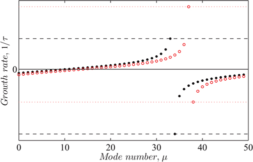
Figure 5.6. Growth and damping rates of different modes in a storage ring with resistive-wall wake fields. In this case, there are 50 bunches in the ring. Positive growth rates indicate unstable (antidamped) modes, and negative growth rates indicate stable (damped) modes. Solid black points show the growth or damping rates of different modes in the case that the betatron tune is 16.2—the integer part of the tune determines which mode has the fastest growth or damping rate. The fact that the fastest mode (number 34) in this case is a damped mode follows from the fact that the fractional part of the tune is less than 0.5. The red circles show the growth or damping rates in the case that the betatron tune is 12.8. The fastest mode is now mode number 37, and because the fractional part of the tune is greater than 0.5, this mode is an antidamped mode. The horizontal black dashed and red dotted lines show the maximum growth and damping rates for the cases with tune 16.2 and 12.8, respectively. The variation of the growth or damping rate with mode number is characteristic of the wake fields present in the storage ring (in this case, resistive-wall wake fields).
Download figure:
Standard image High-resolution imageIn an electron storage ring for a third-generation synchrotron light source, resistive-wall wake fields can drive coupled-bunch modes with growth times of hundreds or tens of turns. In practice, beams may be stable at low beam current because synchrotron radiation and decoherence provide natural damping mechanisms that can be strong enough to suppress the instability. However, as more current is injected into the ring, the wake fields eventually become strong enough for the beam to be unstable; the oscillations of individual bunches will then grow in amplitude until some particles are lost from the beam, reducing the current and restoring beam stability. This means that coupled-bunch instabilities can appear as a current limit in machine operation, preventing the injection of beam currents larger than the threshold for instability set by the wake fields.
To achieve the performance specifications of the storage ring, however, it may be necessary to operate with beam currents significantly larger than the instability threshold. In that case, it is possible to use a bunch-by-bunch feedback system to maintain beam stability [27–29]. In its simplest form, a bunch-by-bunch feedback system consists of a beam position monitor (BPM) capable of detecting the co-ordinates of each bunch on each turn, a high-power amplifier, and a fast kicker that can deflect each bunch in the beam as it passes (see figure 5.7). In principle, the signal from the BPM can be amplified and fed to the kicker so that any bunch with some transverse offset from the closed orbit is deflected back towards the closed orbit. Usually, the correction to each bunch trajectory needs to be done gradually over some number of turns because of limitations in the technology of the feedback system. For example, causality can prevent the signal detected on one turn being fed back to a given bunch on the same turn, because the bunches are travelling at close to the speed of light. Although this limitation may be overcome, in principle, by arranging for the feedback signal to take a shorter path from the BPM to the kicker than the beam (across a diameter of the storage ring, for example), amplification and processing of the signal inevitably introduces some delay in the system. Nevertheless, bunch-by-bunch feedback systems can be constructed and operated to provide damping of coherent betatron (and synchrotron) oscillations, with damping times of some tens of turns [30, 31]. This is usually sufficient to maintain beam stability in the parameter regimes needed by modern light sources and colliders. It should be mentioned, however, that the first mitigation to consider is normally to minimise the wake fields as far as possible. For resistive-wall wake fields, this means (for example) having a beam pipe with a large diameter, and using a material with a good electrical conductivity, such as aluminium or copper. However, long-range wake fields can also come from other sources, such as cavities and transitions in the vacuum chamber, and each section of the vacuum chamber needs to be carefully designed to minimise the wake fields that will be generated by the beam in that section.
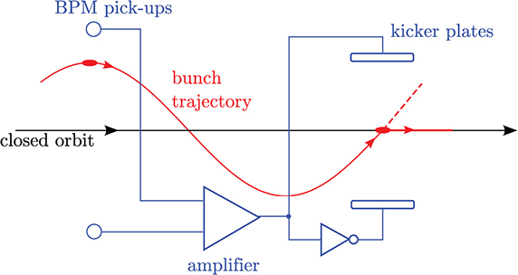
Figure 5.7. Principle of a fast feedback system for damping coupled-bunch instabilities. The signal from a bunch passing through a BPM is amplified and used to control the deflection applied by a kicker. If the phase advance from the BPM to the kicker is an odd multiple of π/2, the bunch is deflected towards the closed orbit. Because of practical limitations from the strength of the kicker, the speed of the amplifier and the level of noise in the system, the correction cannot be achieved in a single pass, but must be applied over several turns of the ring.
Download figure:
Standard image High-resolution imageReferences
- [1]Roqué X 1991 Møller scattering: a neglected application of early quantum electrodynamics Arch. Hist. Exact Sci. 44 197–264
- [2]Piwinski A 1974 Intra-beam scattering Proc. 9th Int. Conf. on High Energy Accelerators (Stanford, CA, USA) pp 405–8.
- [3]Bjorken J D and Mtingwa S K 1983 Intrabeam scattering Part. Accel. 13 115–43
- [4]Kubo K and Oide K 2001 Intrabeam scattering in electron storage rings Phys. Rev. Spec. Top. - Accel. Beams 4 124401
- [5]Kubo K et al 2002 Extremely low vertical emittance beam in the Accelerator Test Facility at KEK Phys. Rev. Lett. 88 194801
- [6]Steier C, Robin D, Wolski A, Portmann G and Safranek J 2003 Coupling correction and beam dynamics at ultralow vertical emittance in the ALS Proc. 2003 Particle Accelerator Conference (Portland, OR, USA) pp 3213–5.
- [7]Bernardini C, Corazza G F, Di Giugno G, Ghigo G, Haissinski J, Marin P, Querzoli R and Touschek B 1946 Lifetime and beam size in a storage ring Phys. Rev. Lett. 10 407–9
- [8]Wiedemann H 2015 Particle Accelerator Physics 4th edn (New York: Springer)
- [9]Conte M and Mackay W W 2008 An Introduction to the Physics of Particle Accelerators 2nd edn (Singapore: World Scientific)
- [10]Wolski A 2014 Beam Dynamics in High Energy Particle Accelerators (London, UK: Imperial College Press)
- [11]Franchetti G 2017 Space charge in circular machines Proc. CERN Accelerator School, Intensity Limitations in Particle Beams (Geneva, Switzerland) , ed H Wernernumber CERN-2017-006-SP pp 353–90
- [12]Zimmermann F 2013 Ion trapping, beam-ion instabilities, and dust Handbook of Accelerator Physics and Engineering 2nd edn , ed A Wu Chao, K H Mess, M Tigner and F Zimmermann (Singapore: World Scientific) pp 159–63
- [13]Nagaoka R 2017 Ions Proc. CERN Accelerator School, Intensity Limitations in Particle Beams (Geneva, Switzerland) , ed H Wernernumber CERN-2017-006-SP pp 519–56
- [14]Wu Chao A 1993 Physics of Collective Beam Instabilities in High Energy Accelerators (New York: Wiley)
- [15]Dohlus M and Wanzenberg R 2017 An introduction to wake fields and impedances Proceedings of the CERN Accelerator School, Intensity Limitations in Particle Beams, number CERN-2017-006-SP, , ed W Herr (Geneva, Switzerland: ) pp 15–41
- [16]Gluckstern R L and Kurennoy S S 2013 Impedance calculation, frequency domain Handbook of Accelerator Physics and Engineering 2nd edn , ed A Wu Chao, K H Mess, M Tigner and F Zimmermann (Singapore: World Scientific) pp 243–8
- [17]Gjonaj E and Weiland T 2013 Impedance calculation, time domain Handbook of Accelerator Physics and Engineering 2nd edn , ed A Wu Chao, K H Mess, M Tigner and F Zimmermann (Singapore: World Scientific) pp 248–52
- [18]Ng K Y and Bane K 2013 Explicit expressions of impedances and wake functions Handbook of Accelerator Physics and Engineering 2nd edn , ed A Wu Chao, K H Mess, M Tigner and F Zimmermann (Singapore: World Scientific) pp 252–62
- [19]Suzuki T 2013 Definitions and properties of impedances and wake functions Handbook of Accelerator Physics and Engineering 2nd edn , ed A Wu Chao, K H Mess, M Tigner and F Zimmermann (Singapore: World Scientific) pp 242–3
- [20]Lumpkin A H, Chang B X and Chae Y C 1997 Observations of bunch-lengthening effects in the APS 7-GeV storage ring Nucl. Instrum. Methods Phys. Res. Sect. A 393 50–4
- [21]Cai Y, Flanagan J, Fukuma H, Funakoshi Y, Ieiri T, Ohmi K, Oide K and Suetsugu Y 2009 Potential-well distortion, microwave instability, and their effects with colliding beams at KEKB Phys. Rev. Spec. Top. - Accel. Beams 12 061002
- [22]Haissinski J 1973 Exact longitudinal equilibrium distribution of stored electrons in the presence of self-fields Il Nuovo Cimento B 18 72–82
- [23]Keil E and Schnell W 1969 Concerning longitudinal instability in the ISR Technical Report CERN–ISR–TH–RF/69–48 (Geneva, Switzerland: CERN)
- [24]Landau L 1946 On the vibration of the electronic plasma J. Phys. (USSR) 10 pp 25–34
- [25]Werner H 2017 Introduction to Landau damping Proc. CERN Accelerator School, Intensity Limitations in Particle Beams (Geneva, Switzerland) , ed W Herrnumber CERN-2017-006-SP pp 137–64
- [26]Boussard D 1975 Observation of microwave longitudinal instabilities in the CPS Technical Report LABII/RF/Int./75–2 (Geneva, Switzerland: CERN)
- [27]Lonza M 2009 Multi-bunch feedback systems Proc. CERN Accelerator School, Synchrotron Radiation and Free Electron Lasers (Dourdan, France), number CERN–2009–005, pp 467–511
- [28]Lonza M 2017 Multi-bunch feedback systems Proc. CERN Accelerator School, Intensity Limitations in Particle Beams (Geneva, Switzerland) , ed W Herrnumber CERN-2017-006-SP pp 471–514
- [29]Fox J D 2013 Feedback to control coupled-bunch instabilities Handbook of Accelerator Physics and Engineering 2nd edn , ed A W Chao, K H Mess, M Tigner and F Zimmermann (Singapore: World Scientific) pp 628–36
- [30]Fox J D, Larsen R, Prabhakar S, Teytelman D, Young A, Drago A, Serio M, Barry W and Stover G 1999 Multi-bunch instability diagnostics via digital feedback systems at PEP-II, DAΦNE, ALS and SPEAR Proc. 1999 Particle Accelerator Conference (New York) pp 636–40
- [31]Fox J D, Mastorides T, Rivetta C, Van Winkle D and Teytelman D 2008 Lessons learned from PEP-II LLRF and longitudinal feedback. Proc. Eleventh European Particle Accelerator Conference (Genoa, Italy) pp 1953–1955
