The basic physics of lasers
Published September 2019
•
Copyright © 2019 Morgan & Claypool Publishers
Pages 1-1 to 1-16
You need an eReader or compatible software to experience the benefits of the ePub3 file format.
Download complete PDF book, the ePub book or the Kindle book
Permissions
Abstract
Chapter 1 begins with a description of how optical photons are produced by different sources, including incandescent lamps, fluorescent lamps and gas discharge tubes. Then the details of electronic transitions that give rise to elemental line spectra and molecular spectra from gas discharge tubes are presented. The properties of laser light, including coherence, monochromaticity and intensity, are reviewed. The formation of a population inversion and the resulting stimulated emission processes as well as the formation of a resonant cavity are explained.
1.1. Introduction
The term laser is an acronym for 'light amplification by stimulated emission of radiation'. The first laser was constructed in 1960 by Thomas Maiman on the basis of theoretical work by Charles Townes and Arthur Schawlow. The operation of the laser follows from the same basic principles as its predecessor, the maser (microwave amplification by stimulated emission of radiation). The name laser was originally used to describe devices that worked in the visible portion of the electromagnetic spectrum. However, the term 'light' in its name is now used in a broader sense to indicate any frequency of electromagnetic radiation. Hence, devices which work in the non-visible part of the spectrum are sometimes called 'x-ray lasers', 'ultraviolet lasers', 'infrared lasers', etc as appropriate, although the term maser is still used for devices that operate in the microwave region. The present book deals primarily with optical lasers.
Lasers are distinguished from other sources of light by the fact that the light that they emit is coherent, that is the electromagnetic fields associated with the various photons in the beam are in phase. More precisely, they have a long coherence length, meaning that the beam remains coherent for a large spatial distance. The fact that the light from a laser is coherent means that it can be very intense and directional, and it also requires that the light be polarized and monochromatic. While 'monochromatic' would imply a single frequency or wavelength, it is necessary to consider the extent to which light needs to be monochromatic in order to satisfy the coherence condition.
We begin by considering the ways in which visible light can be produced and how the production method affects the degree of monochromaticity.
1.2. Optical spectra
Optical photons are most commonly emitted by materials as a result of electronic processes in the material and can be classified in terms of those which produce a broad distribution of wavelengths and those which are, more-or-less, monochromatic. Analogous to the situation which produces x-rays by bremsstrahlung, thermal energy results in the emission of photons with a broad distribution of wavelengths, or a continuum spectrum. This is black body radiation and the wavelength of the maximum in the energy spectrum, in nm, is given by Wein's displacement law as

where T is the temperature in Kelvin and b is the displacement constant 2.8978 × 10⁶ K nm. An incandescent lamp produces light that is a good approximation of black body radiation as illustrated in figure 1.1 where the maximum in the spectrum at about 660 nm corresponds to a temperature of approximately 4400 K. As the visible portion of the electromagnetic spectrum covers the range of wavelengths from about 390 to 700 nm, the figure shows that the incandescent lamp emits most of its radiation in the infrared portion of the spectrum.

Figure 1.1. Spectra of incandescent, halogen and fluorescent lamps. AM 1.5 is the spectrum of simulated natural daylight. (Figure 2 reprinted from Virtuani et al 2006. Copyright (2006), with permission from Elsevier.)
Download figure:
Standard image High-resolution imageAnalogous to the discrete line spectra of x-ray sources which are the result of specific electronic transitions, well defined spectral lines in the optical region can also result from electronic transitions. Because optical photons are of much lower energy than x-ray photons, the electronic transitions involve outer shell electrons with small binding energies, rather than inner shell electrons, as is the case for x-ray production. The common fluorescent lamp produces spectra which contain well defined peaks, as illustrated in figure 1.1.
A quantitative example of optical line spectra follows from the calculated energy levels of a hydrogen atom, as illustrated in figure 1.2. The transitions are identified by the energy level of the final (lowest) level involved in the transition and are named after researchers who studied optical spectroscopy in the early 20th century. The energy, E, of the photon that is emitted is given as

where n2 is the quantum number for the initial (higher energy) state and n1 is the quantum number for the final (lower energy) state. The wavelength of the emitted photons is related to the energy of the transition by

When the energy is in eV and the wavelength is in nm, then the constant h.c. = 1.24 × 10³ eV nm. The range of visible wavelengths corresponds to a range of energies from 3.18 to 1.77 eV. The Lyman series involves transitions that end at the ground state (n1 = 1) and produce photons in the far ultraviolet. It is some of the Balmer series transitions (which end at n1 = 2) that have energies corresponding to optical photons.

Figure 1.2. The electronic energy levels in atomic hydrogen showing some of the transitions that give rise to photon emission. The names of the various series of transitions are indicated. Szdori / wikimedia commons / CC-BY-SA 3.0 / https://creativecommons.org/licenses/by-sa/3.0/deed.en https://commons.wikimedia.org/wiki/File:Hydrogen_transitions.svg.
Download figure:
Standard image High-resolution imageA typical discharge tube for producing emission spectra from a gas is illustrated in figure 1.3. A high voltage discharge excites electrons from their ground state to excited levels. These excited levels are unstable and will spontaneously decay back to a lower energy excited state or the ground state, thereby emitting energy in the form of photons.
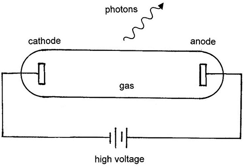
Figure 1.3. Typical gas discharge tube for producing line spectra.
Download figure:
Standard image High-resolution imageIn cases where an atom is part of a molecule, then the details of the electronic energy
levels become more complex. The energy of the system is not only a result of the energy
of the electrons in their quantized energy levels but also results from the rotational
and vibrational energy associated with the molecule. These rotational and vibrational
levels are quantized, where the rotational levels are assigned a quantum number
J and the vibrational levels are assigned a quantum number
![$\mathit{\unicode[Book Antiqua]{x76}}$](https://content.cld.iop.org/books/10__1088_2053-2571_ab2f2f/revision2/bk978-1-64327-696-0ch1ieqn5.gif) . Figure 1.4 shows possible transitions involving
rotational and vibrational energy levels. Transitions that involve a change in
vibrational state, but do not involve a change in rotational state (i.e.
ΔJ = 0), are referred to as 'Q' transitions. Transitions that involve
a change of vibrational state as well as a decrease by one unit of rotational energy
(i.e. ΔJ = −1) are referred to as 'P' transitions, while those which
involve an increase in rotational energy (i.e. ΔJ = +1) are called 'R'
transitions. These are identified in figure 1.4.
. Figure 1.4 shows possible transitions involving
rotational and vibrational energy levels. Transitions that involve a change in
vibrational state, but do not involve a change in rotational state (i.e.
ΔJ = 0), are referred to as 'Q' transitions. Transitions that involve
a change of vibrational state as well as a decrease by one unit of rotational energy
(i.e. ΔJ = −1) are referred to as 'P' transitions, while those which
involve an increase in rotational energy (i.e. ΔJ = +1) are called 'R'
transitions. These are identified in figure 1.4.
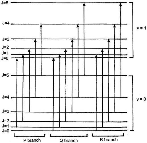
Figure 1.4. Transitions involving vibrational states (designated with the quantum number
![$\mathit{\unicode[Book Antiqua]{x76}}$](https://content.cld.iop.org/books/10__1088_2053-2571_ab2f2f/revision2/bk978-1-64327-696-0ch1ieqn1.gif) ) and rotational states (designated with
the quantum number J).
) and rotational states (designated with
the quantum number J).
Download figure:
Standard image High-resolution imageFigure 1.5 shows the measured spectrum for N2O and illustrates the P-branch, Q-branch and R-branch of the spectrum. It is common to label the horizontal axis of such spectra with the wavenumber (usually in cm−1). As the figure shows, the spectral peaks occur for wavenumbers around 600 cm−1. The wavenumber in cm−1 may be expressed in units of energy using the relation that a photon of wavenumber 1 cm−1 has the energy of a photon with a wavelength of 1 cm. This relationship is given in equation (1.3) when the constant is expressed in appropriate units h.c. = 1.24 × 10⁻⁴ eV cm. Thus, a wavenumber of 1 cm−1 corresponds to an energy of 1.24 × 10⁻⁴ eV and a wavenumber of 600 cm−1 corresponds to an energy of (1.24 × 10⁻⁴ eV cm) × (600 cm−1) = 0.074 eV. The wavelength in cm is merely the inverse of the wavenumber in cm−1, thus a wavenumber of 600 cm−1 will give a wavelength of (600 cm−1)−1 = 1.67 × 10⁻³ cm = 1.67 × 10⁴ nm.
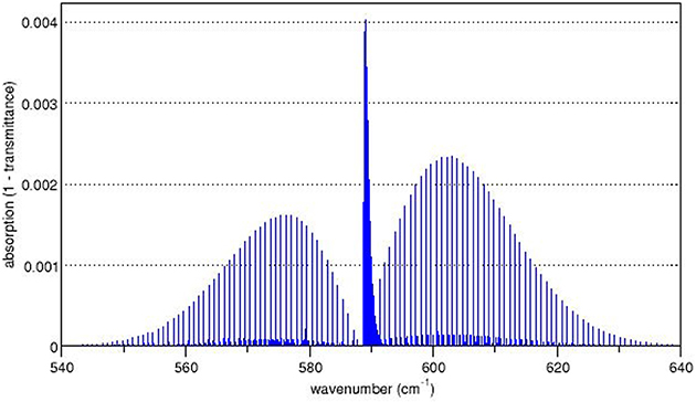
Figure 1.5. Rotational/vibrational spectrum of N2O. Petergans / wikimedia commons / CC-BY-SA 3.0 / https://creativecommons.org/licenses/by-sa/3.0/deed.en https://en.wikipedia.org/wiki/Rotational%E2%80%93vibrational_spectroscopy#/media/File:Nu2_nitrous_oxide.png.
Download figure:
Standard image High-resolution imageA comparison of figures 1.4 and 1.5 shows that the P-branch has the lowest energy and, therefore, appears on the left side of the spectrum. The Q-branch gives rise to the peak at the center of the spectrum. The R-branch corresponds to the right-hand portion of the spectrum.
The rotational/vibrational spectrum of N2O spectrum illustrates an interesting feature that is often seen in such spectra. The P- and R-branches show the presence of a weak spectral component superimposed on the principal spectrum. Nitrogen consists of two naturally occurring isotopes, 14N (about 99.7%) and 15N (about 0.3%). These two isotopes have different masses and give rise to molecules with different moments of inertia. Thus, the splitting of the energy levels is slightly different for molecules which contain atoms of different nitrogen isotopes and this results in two superimposed spectra.
Figure 1.6 shows the rotational/vibrational spectrum of HCl. It is clear in this figure that the P- and R-branches appear, as expected, but the Q-branch is missing. For a linear molecule consisting of two elements, A and B, of composition AB, quantum mechanical selection rules forbid transitions with ΔJ = 0, thereby eliminating the Q-branch.

Figure 1.6. Rotational/vibrational spectrum of HCl. CC-BY-SA 4.0. Physics Libretexts.org https://phys.libretexts.org/TextBooks_and_TextMaps/University_Physics/Book%3A_University_Physics_(OpenStax)/Map%3A_University_Physics_III_-_Optics_and_Modern_Physics_(OpenStax)/9%3A_Condensed_Matter_Physics/9.2%3A_Molecular_Spectra.
Download figure:
Standard image High-resolution image1.3. Stimulated emission
The previous section has shown how electronic transitions in atoms and molecules that involve discrete quantized energy levels can give rise to well defined spectral wavelengths. While this feature will satisfy, more-or-less, the requirement that a light source produces photons that are monochromatic in order to be classified as a laser, we still need to consider the nature of the electronic transition and the question of polarization. Here we begin with a consideration of the difference between spontaneous emission processes and stimulated emission processes.
Figure 1.7 shows a diagram of a spontaneous emission process. In figure 1.7(a), energy (in this case in the form of a photon) is absorbed by an atom, giving rise to the excitation of one of its electrons. As this excited state is not stable it will, after some time, decay back to the ground state as in figure 1.7(b) re-emitting a photon with energy equal to the difference in the energies of the excited and ground states.
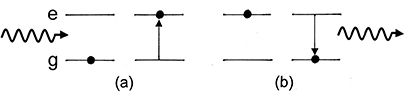
Figure 1.7. Spontaneous emission process; (a) excitation of an atom into an excited state and (b) spontaneous decay back to the ground state accompanied by photon emission.
Download figure:
Standard image High-resolution imageFigure 1.8 illustrates a stimulated emission process. As in the spontaneous emission process, an atom absorbs energy, it is excited, and this excited state decays spontaneously, re-emitting a photon. This re-emitted photon encounters another atom of the same type which is in the excited state and which has not yet decayed spontaneously. The incident photon causes the excited atom to decay before it would have decayed spontaneously. As the two atoms involved are of the same type, they have the same energy levels, and the incident photon and the photon that results from the stimulated emission, will have the same energy (within certain limits, as discussed further below). There are two additional features that are of importance in this process; the two photons are not only of the same energy, but they are in phase and have the same polarization vector. Thus, they satisfy the description of radiation from a laser.
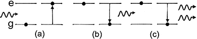
Figure 1.8. Stimulated emission process: (a) absorption of a photon and excitation of electron into excited state, (b) spontaneous decay and emission of photon from unstable excited state and (c) stimulated emission of photon from another atom in an excited state by photon from spontaneous decay in panel (b).
Download figure:
Standard image High-resolution imageThe characteristics of the radiation as described above are that it is monochromatic (to the degree discussed below) and it is intense, as the components of the beam are all in phase and interfere constructively with each other. If this process continues from a collection of the same type of atoms, then the beam will continue to increase in intensity. Light, in which the components of the beam remain in phase with one another over an extended distance, is referred to as coherent.
Two practical problems need to be resolved in order to create the situation as described above. Firstly, we need to ensure that there are a sufficient number of atoms in the excited state (rather than in the ground state) for the stimulated emission to occur frequently, and we need to ensure that there is sufficient opportunity for the beam to gain strength by successive stimulated emissions. The solutions to these two problems are the creation of a population inversion and the creation of an appropriate resonant cavity, respectively. These two requirements are discussed below.
1.4. Creating a population inversion
Consider a simple two-level quantum system as illustrated in figure 1.9(a). At zero temperature all atoms will be in their ground state. However, at any temperature, T, above absolute zero, thermal effects need to be considered. The distribution of particle velocities as a function of temperature is given by the Maxwell–Boltzmann distribution as illustrated in figure 1.10. This distribution has the functional form

where
![$f(\mathit{\unicode[Book Antiqua]{x76}})$](https://content.cld.iop.org/books/10__1088_2053-2571_ab2f2f/revision2/bk978-1-64327-696-0ch1ieqn7.gif) is the fraction of atoms with velocity
is the fraction of atoms with velocity
![$\mathit{\unicode[Book Antiqua]{x76}}$](https://content.cld.iop.org/books/10__1088_2053-2571_ab2f2f/revision2/bk978-1-64327-696-0ch1ieqn8.gif) and kB is the
Boltzmann constant. The Maxwell–Boltzmann function may also be expressed as a
distribution in energy using a change of variables and the relation E =
mv2/2, as
and kB is the
Boltzmann constant. The Maxwell–Boltzmann function may also be expressed as a
distribution in energy using a change of variables and the relation E =
mv2/2, as

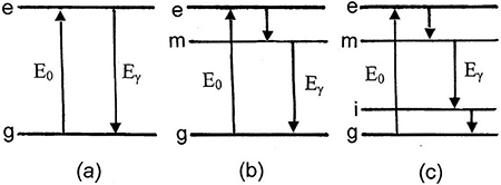
Figure 1.9. (a) Two-level system showing energy absorption, E0, and emission, Eγ, between the ground state (g) and the excited state (e). (b) Three-level system showing energy absorption between the ground state (g) and the excited state (e), the spontaneous emission between the excited state (e) and a metastable state (m) and stimulated emission between the metastable state (m) and the ground state (g). (c) Four-level system showing absorption between the ground state (g) and excited state (e), the spontaneous emission between the excited state (e) and the metastable state (m), stimulated emission between the metastable state (m) and the intermediate state (i) and spontaneous emission between the intermediate state (i) and the ground state (g).
Download figure:
Standard image High-resolution image
Figure 1.10. Maxwell–Boltzmann distributions at different temperatures.
Download figure:
Standard image High-resolution imageFor a system consisting of discrete microstates with energies Ei , then the number of atoms in a state with energy Ei follows from the Maxwell–Boltzmann distribution as

where N is the total number of atoms in the system. A plot of equation (1.6) at room temperature is shown in figure 1.11. It is clear that the state population decreases as a function of increasing energy. This is the normal equilibrium situation. For a population inversion we require that the population of a particular energy level is greater than that for the level below it. For the case in figure 1.9(a) atoms in the ground state can be excited into the higher energy state by inputting an energy greater than the excited state energy, E0. This can be done by, e.g., photon irradiation or an electric discharge. Excited state atoms will spontaneously decay back to the ground state with a characteristic time (the mean life of the excited state) releasing energy in the form of a photon of energy Eγ = E0. If a sufficient number of atoms are excited from the ground state in less than the mean life of the excited state, a population inversion results and stimulated emission can occur. However, this population inversion cannot be maintained as stimulated emissions will decrease the population of the excited state and increase the population of the ground state until the population inversion is eliminated.
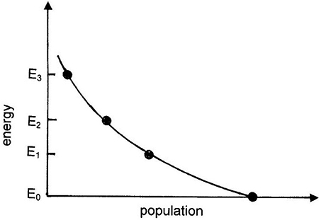
Figure 1.11. Population as a function of energy for the Maxwell–Boltzmann distribution near room temperature.
Download figure:
Standard image High-resolution imageThe simplest system which is compatible with the requirements for the design of an operational laser is the three-level system, as shown in figure 1.11(b). The short-lived (e.g., ∼10−8 s) excited state decays spontaneously to a metastable state at a lower energy which in turn decays by stimulated emission to the ground state. The metastable state is relatively long-lived (e.g., 10−5−10−4 s). Thus, ground state atoms are pumped up to the excited state which quickly decays to the metastable state, where atoms collect to create a population inversion with the ground state. Three-level lasers most commonly operate in a pulsed mode; a short discharge from a flash tube, for example, pumping the system up to the excited state from the ground state followed by the stimulated emission from the metastable state. It should be noted that the energy (per photon) required to excite the ground state atoms up into the excited state is greater than the energy (per photon) produced by the stimulated decay. This means, for example, that green photons might be needed to excite the transition to the excited state while red photons might be emitted during the stimulated decay process.
Lasers that operate continuously are more commonly based on a four-level system, as shown in figure 1.9(c). In this case, atoms that are pumped up to the excited state decay quickly by spontaneous emission to the relatively long-lived metastable state. Atoms collect in this metastable state and then decay by stimulated emission to a short-lived intermediate state, which quickly decays back to the ground state. Since the intermediate state decays quickly, its population remains small. The population inversion can, therefore, be maintained between the metastable state and the intermediate state and the excited state can continuously be populated by excitation of ground state atoms.
1.5. Laser modes and coherence
The second consideration in laser design is the creation of a resonant cavity so that the beam can be amplified by continuous constructive interference of the beam components. Figure 1.12 shows the basic design of a resonant cavity. The cavity has a fully reflecting mirror on one end and a partially reflecting mirror on the other end. Photons that are emitted as a result of a stimulated decay process are reflected, back and forth in the cavity, causing more stimulated decays, which produce more photons, all of which are of the same energy and are in phase with one another. Some of the coherent radiation leaks out of the partially reflecting mirror and constitutes the laser beam.
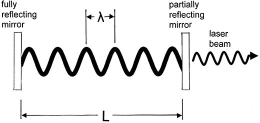
Figure 1.12. Conditions for creating a resonant laser cavity which is a half integer number of wavelengths long.
Download figure:
Standard image High-resolution imageThe above process sounds quite simple, but there is a serious concern; how do we maintain the phase relationship of the waves that are reflected from the ends of the cavity? In order to do this, it is necessary to produce a resonant cavity that is a half integer number of wavelengths in length. That is, we want to create a condition where the waves inside the cavity are standing waves. Figure 1.12 illustrates this point. For this condition to be met we require that

where n is an integer, λ is the wavelength of the radiation and L is the length of the cavity. Actually, figure 1.12 is not really to scale, as a typical wavelength would be in the range of a few hundred nanometers and a typical cavity would have a length in the centimeter or many-centimeter range. Using L = 30 cm and λ = 500 nm, gives (3 × 10⁻¹ m)/(2.5 × 10−7 m) = 1.2 × 10⁶ half wavelengths in the cavity. If we think about how we might actually create this situation, we realize that it is a very difficult task. The light, which has a wavelength of the order of a few hundred nanometers, bounces back and forth in the cavity many times. Any error in satisfying relationship (1.7) will be compounded with each reflection. Therefore, we might think that we need to know how accurately equation (1.7) has to be satisfied in order to make a functioning laser. Fortunately, we never actually have to concern ourselves with this problem, and that brings us back to a question we have never really answered; how monochromatic is monochromatic?
The decay of a quantum mechanical state is a statistical process characterized by a characteristic mean decay time, τ. As the exact time of the decay is uncertain, the energy of the state will be uncertain with a distribution that is related to the mean time by the Heisenberg uncertainty principle,

or

This form of the Heisenberg uncertainty principle follows directly from the more common form involving position, x, and momentum, p;

by the relationships for
position, velocity,
![$\mathit{\unicode[Book Antiqua]{x76}}$](https://content.cld.iop.org/books/10__1088_2053-2571_ab2f2f/revision2/bk978-1-64327-696-0ch1ieqn15.gif) , and time, t;
, and time, t;

and momentum and energy, E,

where m is mass. Taking the differential of equations (1.11) and (1.12) and substituting into equation (1.10) gives the form of the uncertainty relation in equation (1.9).
Using τ = 10−5 s for a metastable state mean lifetime in
equation (1.9), we
find ΔE
 3 × 10⁻¹¹ eV, out of a photon
energy of about 2.5 eV (for λ = 500 nm). This value is actually a
substantial underestimate of the actual width of the energy distribution as thermal
effects substantially broaden the distribution. In a gas, this broadening results from
Doppler effects due to the thermal motion. In a solid, phonon interactions broaden the
energy distribution. In many materials, an energy width of around 10−5 eV is
fairly typical. Since
3 × 10⁻¹¹ eV, out of a photon
energy of about 2.5 eV (for λ = 500 nm). This value is actually a
substantial underestimate of the actual width of the energy distribution as thermal
effects substantially broaden the distribution. In a gas, this broadening results from
Doppler effects due to the thermal motion. In a solid, phonon interactions broaden the
energy distribution. In many materials, an energy width of around 10−5 eV is
fairly typical. Since

then it is straightforward to show that

From the above example, we find Δλ ∼ 2 × 10⁻³ nm. This is still small compared to the wavelength of 500 nm, so the photons are monoenergetic to about 1 part in (500 nm)/(2 × 10−3 nm) = 2.5 × 10⁵.
It is now necessary to consider the resonant modes of the cavity. We need to ask: if the cavity contains n half wavelengths, then how much does the wavelength have to change to fit n + 1 half wavelengths in the cavity? From equation (1.7) we solve for λ:

and differentiating gives

So, for Δn = 1, then Δλ = 4 × 10⁻⁴ nm. Comparing this with the typical width of the wavelength distribution from the stimulated emission shows that there are about five cavity modes within this distribution. This relationship is illustrated in figure 1.13.

Figure 1.13. Relationship of wavelength distribution from stimulated emission and resonant cavity modes in a typical laser. Dr Wolfgang Geithner / wikimedia commons / CC BY SA 3.0 https://creativecommons.org/licenses/by-sa/3.0/deed.en.
Download figure:
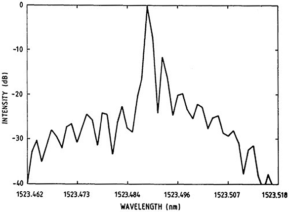
Standard image High-resolution imageThe above analysis shows that, in a typical situation, it is not necessary to adjust the length of the resonant cavity to match the wavelength of the lasing transition. No matter what the length of the cavity is, it will contain several resonant modes. A measured wavelength spectrum of a laser transition is illustrated in figure 1.14. Thus, the monochromatic light produced by a laser typically consists of a number of closely spaced modes within a Gaussian-like envelope. In the next two chapters we describe the principle of operation of several common types of lasers.
Figure 1.14. Wavelength spectrum of the lasing transition at 1523 nm (infrared) from a He–Ne laser showing the presence of cavity modes. Reprinted with permission from Junttila and Stahlberg 1990 © The Optical Society.
Download figure:
Standard image High-resolution image
1.6. Problems
- 1.1.A laser with a lasing cavity of 0.2 m in length produces light with a wavelength of 550 nm. If the lifetime of the lasing transition is very long, then the Heisenberg linewidth of the energy distribution of the laser state will be very narrow and the resonant cavity modes will not exist. Calculate the maximum lifetime of the lasing state that is consistent with the construction of a laser.
- 1.2.
- (a)Calculate the spacing in energy (in eV) and in wavelength (in nm) between the resonant cavity modes of a laser operating at 600 nm with a cavity length of 1.0 m.
- (b)Repeat part (a) for a cavity length of 0.001 m.
- 1.3.Consider a hypothetical laser consisting of 1020 atoms of lasing material.
- (a)If the system has three energy levels with energies of −10.0 eV, −9.8 eV and −9.4 eV, find the equilibrium populations of the three levels according to Maxwell–Boltzmann statistics at room temperature.
- (b)Repeat part (a) if the lasing material is heated to 5000 K.
References
- Csele M 2004 Fundamentals of Light Sources and Lasers (Hoboken, NJ: Wiley)
- Hecht J 1992 The Laser Guidebook 2nd edn (New York: McGraw Hill)
- Junttila M L and Stahlberg B 1990 Laser wavelength measurement with a Fourier transform wavemeter Appl. Opt. 29 3510–16
- Silfvast W T 1996 Laser Fundamentals (Cambridge: Cambridge University Press)
- Svelto O 1998 Principles of Lasers 4th edn (New York: Springer)
- Virtuani A, Lotter E and Powalla M 2006 Influence of the light source on the low-irradiance performance of Cu(In,Ga)Se2 solar cells Sol. Energy Mater. Sol. Cells 90 2141–9
- Wilson J and Hawkes J F B 1987 Lasers: Principles and Applications (New York: Prentice Hall)