
Modelling markets as ecosystems with the help of maximum entropy
Published November 2022
•
Copyright © IOP Publishing Ltd 2022
Pages 7-1 to 7-26
You need an eReader or compatible software to experience the benefits of the ePub3 file format.
Download complete PDF book, the ePub book or the Kindle book

Permissions
Abstract
The final chapter 7 addresses the so-called 'Marshall's problem', namely integrating physics and biology into economics in a way that both contains its orthodox core as well as provides a transdisciplinary perspective on economic complexity. This is a main theme of this book which completes the puzzle. We propose a method based on the replicator dynamics (discussed in chapter 4) as an equation to model natural selection in markets. A main difficulty is how to obtain the payoff matrix connecting the pairwise effects between interacting market entities. We thus use the pairwise maximum-entropy procedure to estimate the payoff matrix. The resulting method is called replicator dynamics pairwise maximum entropy (RDPME). We test the forecasting performance of RDPME using daily market values from 2014 to 2019 of America's top revenue companies.
'Investing should be dull, like watching paint dry or grass grow. If you want excitement, take $800 and go to Las Vegas.'
—Paul Samuelson
We start with a short history of different attempts of modelling the dynamics of markets and of finding a law for the price fluctuations. We briefly review the conceptual path from Louis Bachelier's theory of Brownian motion to the modern efficient-market hypothesis (EMH), which states that asset prices reflect all available information and, as a consequence, it is impossible to 'beat the market' consistently.
Next we discuss the criticism to the EMH. One alternative economic theory to EMH is the adaptive market hypothesis (AMH), which extends the main tenets of the controversial EMH by applying the principles of evolution and behavior to financial interactions.
Then we move onto the aim of this chapter which is, by adopting the AMH point of view, to develop a method of market dynamics forecasting that combines different previously discussed concepts of physics, biology and economics. This method is based on the replicator dynamics (RD) (discussed in chapter 4) as an equation to model natural selection in markets. A main difficulty is how to obtain the payoff matrix connecting the pairwise effects between interacting market entities. Thus we use the pairwise maximum-entropy (PME) procedure (introduced in chapter 5) to estimate the payoff matrix. The resulting method is called replicator dynamics pairwise maximum entropy (RDPME).
To test the method, daily market values from 2014 to 2019 of America's top revenue companies are used. As it is customary in time series forecasting analysis, these series are divided into a training period, used to infer the RDPME parameters (intrinsic growth rates and payoff matrix), and a validation period, used to validate the model. Different partitions into training and validation periods are considered.
We show that the RDPME method outperforms the stochastic benchmark of the geometric random walk in predicting empirical shares xi for most of the companies along most choices of validation periods (although the mean relative errors of the RDPME are in general only modestly smaller than those produced by the stochastic benchmark).
We conclude this chapter by reviewing some caveats, extensions, and possible future improvements.
7.1. Background: a short history of market modelling
7.1.1. Of pollen motion, drunks and bond prices
The French stock broker Jules Augustin Frédéric Regnault was the first who suggested a modern theory of stock price changes, based on statistical and probabilistic analyses, in his Calcul des Chances et Philosophie de la Bourse (1863). His hypotheses were later used by the French mathematician Louis Bachelier to found the science of investing or mathematical finance with his 1900 doctoral thesis, Théorie de la speculation (The Theory of Speculation). It was an attempt to create a formula to capture the movement of bonds in the Paris Bourse, or stock exchange. Bachelier developed the theory of what we nowadays call Brownian motion , named after the Scottish botanist Robert Brown.
In 1827, Brown was struck by the jittery motion of small particles of pollen floating on the surface of water he observed through a microscope. Since pollen was organic, Brown's first thought was that it might be exhibiting signs of life as it jumped around the surface. But when Brown later saw the pollen's behavior replicated by inorganic matter like coal dust, he ruled out the hypothesis that the effect was life-related. Brown couldn't provide an explanation of this frenetic dance.
In fact, it was Einstein in 1905 who developed the theory for the Brownian motion by modelling the motion of the pollen particles as being displaced by collisions with individual water molecules. The direction of the force of atomic bombardment is constantly changing, and at different times the particle is hit more on one side than another, leading to the seemingly random nature of the motion. Importantly, this explanation of Brownian motion served as convincing evidence that atoms and molecules exist. The many-body interactions that yield the Brownian motion cannot be solved by taking into account every involved molecule. Instead, Einstein adopted a statistical mechanics approach, in terms of a probabilistic description of the molecular effects on the grain of pollen. He arrived at a theory formally identical to the one devised five years earlier by Bachelier for the movement of bonds. So here we have another formal equivalence linking statistical mechanics with finance economics.
When treated as a discrete-space (integers) and discrete-time model, Brownian motion becomes the epitome of a stochastic or random process: the random walk . In other words, essentially, Bachelier's formula tells us that the price of a security rises or falls accordingly to the result of flipping a coin. This random walk is also called the drunkard's walk . The simplest example is one-dimensional; let us imagine a drunkard who exits a bar attempting to return home. He is so intoxicated that he only remembers his house and the bar are both on the same street, but he has no idea whether it is to the left or to the right of the bar. So he starts by arbitrarily choosing the right and giving a step toward this direction. But then he hesitates and before every next step he faces a binary decision: right or left? This concept was introduced into science by Karl Pearson in a letter to Nature in 1905: 'A man starts from a point O and walks l yards in a straight line; he then turns through any angle whatever and walks another l yards in a second straight line. He repeats this process n times.' Pearson then required the probability that after these n stretches the man is at a distance d from his starting point O. Interestingly, the solution to this problem was provided in the same volume of Nature by Lord Rayleigh (1905), who told him that he had solved this problem 25 years earlier when studying the superposition of sound waves of equal frequency and amplitude but with random phases. Pearson concluded that 'The lesson of Lord Rayleigh's solution is that in open country the most probable place to find a drunken man who is at all capable of keeping on his feet is somewhere near his starting point!'
However, Bachelier's theory remained unnoticed gathering dust on library bookshelves for 60 years until the American economist Paul Samuelson discovered it. Samuelson expanded and refined Bachelier's work. As Bachelier did, he also assumed that market prices are the best estimates of value and that price changes follow random patterns, so future news and stock prices are unpredictable. A problem with Bachelier's modelling was that security prices can take negative values, but this is nonsense from a financial point of view. This drawback was overcome by Samuelson (1965a, 1965b) who proposed the so-called Geometric Brownian motion, in which the natural logarithm of the price is assumed to walk a random walk, usually a random walk with drift. That is, the changes in the natural log from one period to the next are assumed to be independent and identically normally distributed.
Therefore, the so-called random walk hypothesis (RWH) (Cootner 1964, Fama 1965, Malkiel 1973) is a financial theory stating that stock market prices evolve according to a random walk (so price changes are random) and thus cannot be predicted.
7.1.2. The efficient market hypothesis and the crypto-trading hamster Mr Goxx
Since prices move as a random walk, Bachelier set forth the revolutionary conclusion that there is no useful information contained in historical price movements of securities. In his own words:
'The mathematical expectation of a speculator is nil' (Bachelier 1900).
Between the time Bachelier proposed his theory and the 1960s when it was rediscovered, the Wall Street Crash of 1929 occurred and a severe worldwide economic depression, the so-called Great Depression, took place during the 1930s. These remarkable economic events stimulated some fruitful investigation. For example, James Case in his 2008 Competition: The Birth of a New Science tells the findings of the American economist and businessman Alfred Cowles III supporting the difficulties of predicting market movements:
'In 1928, he purchased subscriptions to twenty-four of the most widely circulated newsletters and monitored their performance for four eventful years−... To his surprise, Cowles discovered that exactly none of twenty-four publications had managed to foretell either the crash of 1929 or the steady market decline that followed'
This idea that financial market returns are difficult to predict is the basis of the modern efficient-market hypothesis (EMH) (Samuelson 1965a, 1965b, Fama 1970), which states that asset prices reflect all available information and as a consequence that it is impossible to 'beat the market' consistently since market prices should only react to new information. In other words, stocks always trade at their fair value on exchanges, making it impossible for investors to purchase undervalued stocks or sell stocks for inflated prices. Therefore, it should be impossible to outperform the overall market through expert stock selection or market timing. The RWH is consistent with the EMH.
EMH is somehow related with the rational choice theory we discussed in chapter 4, both assume that there is a well-defined model of economic behavior and that rational investors would all follow it. EMH added another step. In the strong version of the theory, financial markets, because they are populated by a multitude of rational and competitive players, would always set prices that reflected all available information in the most accurate possible way.
Proponents of EMH posit that investors benefit from investing in a low-cost, passive portfolio. In fact, data compiled by Morningstar Inc., in its August 2019 Active/Passive Barometer study, supports the EMH. This report measures the performance of U.S. active funds against passive peers in their respective Morningstar Categories. The Active/Passive Barometer spans more than 4000 unique funds that account for approximately $12.5 trillion in assets, or about 64% of the U.S. fund market. Morningstar compared active managers' returns in all categories against a composite made of related index funds and exchange-traded funds (ETFs). The study found that over a 10 year period beginning June 2009, only 23% of active managers were able to outperform their passive rivals (Morningstar 2019).
In addition, while a percentage of active managers do outperform passive funds at some point, the challenge for investors is being able to identify which ones will do so over the long term. Less than 25% of the top-performing active managers can consistently outperform their passive manager counterparts over time (Downey 2021).
Economist Burton Malkiel mocked the financial services industry. He famously quipped, 'A blindfolded monkey throwing darts at a newspaper's financial pages could select a portfolio that would do just as well as one carefully selected by the experts.' Actually, not a monkey but a hamster is currently proving such a claim. And it's not stocks: it's cryptocurrencies. This crypto-trading hamster that goes by the name of Mr Goxx is a social media sensation in Germany. Named after Mt Gox—a Tokyo-based cryptocurrency exchange company founded in 2010 that was responsible for more than 70% of bitcoin transactions at its peak until it was hacked and declared bankruptcy in 2014—the rodent is equipped with a trading office attached to his regular cage. Mr Goxx goes on the wheel where he selects which cryptocurrency he would like to trade by simply spinning it. The office has two tunnels: one for buying and one for selling, and every time he goes through one of them, the desired transaction is completed. The hamster livestreams his crypto tradings on video live streaming service twitch. As of 24 September 2021, the hamster's performance was up more than 16% 1 since it began trading in June 2021 (Protos 2021), an impressive feat for anyone. Bitcoin and the S&P 500 have climbed about 14% and 5% respectively, over the same time period. In other words, the hamster is beating not only bitcoin, but the S&P 500, as well as many professional traders and funds since it started trading.
7.1.3. Criticism to the efficient market hypothesis
There have been several criticisms of EMH. Some of the most common are as follows.
First, real markets exhibit inefficiencies and there are some markets that are less efficient than others. An inefficient market is one in which an asset prices do not accurately reflect their true or fair value. This may occur for several reasons. Market inefficiencies may exist due to information asymmetries, lack of competition, tax distortions, lack of buyers and sellers (i.e., low liquidity), high transaction costs or delays, market psychology, and human emotion, among other reasons (Downey 2021). In particular, psychology and emotions are key drivers of market sentiment. That is, the overall consensus of investors about a stock or the stock market as a whole is not always based on fundamentals. Day traders and technical analysts also rely on market sentiment, as it influences the technical indicators they utilize to measure and profit from short-term price movements often caused by investor attitudes toward a security. In A Study of History, Arnold Toynbee (1946) warns to beware of what he calls the 'apathetic fallacy', whereas 'Ruskin warned his readers against the 'pathetic fallacy' of imaginatively endowing inanimate objects with life', when addressing a system composed of human beings we need to avoid the converse error of blindly applying a scientific method devised for the study of inanimate nature.
Second, Eugene Fama never imagined that his efficient market would be 100% efficient all the time. That would be impossible, as it takes time for stock prices to respond to new information. The EMH, therefore doesn't give a strict definition of how much time prices need to revert to fair value. Third, the EMH assumes a sort of homogeneity of the market participants; i.e., all investors perceive all available information in precisely the same manner. But this is hardly the case. For example, there are many different methods for analyzing and valuing stocks. If one investor focuses on value, and then looks for undervalued market opportunities, while another focuses on growth and evaluates the same stock on the basis of its growth potential, these two investors may arrive at a different assessment of the stock's fair market value. Therefore, since investors value stocks differently, it is impossible to determine what a stock should be worth under an efficient market. Fourth, under the EMH, no investor should ever be able to beat the market or the average annual returns that all investors and funds are able to achieve using their best efforts. This is why proponents of the EMH conclude investors may profit from investing in a low-cost, passive portfolio, i.e., purchasing a representative benchmark, such as the S&P 500 index, and hold it over a long time horizon. But there are many investors who have consistently beaten the market. Warren Buffett is one of those who's managed to outpace the averages year after year (Dhir 2021).
In addition, there is evidence against the RWH for the logarithm of wealth relatives of small-firms portfolios (Lo et al 2002).
7.1.4. Combining efficient market hypothesis with behavioral finance: the adaptive market hypothesis
Opponents of EMH believe that it is possible to beat the market and that stocks can deviate from their fair market values. In particular, behavioral finance challenges the notion that companies always trade at their fair value, pointing out that investors are not always rational and stocks do not always trade at their fair value during financial bubbles, crashes, and crises. Thus behavioral economists attempt to explain stock market anomalies through psychology-based theories. This is the case of the adaptive market hypothesis (AMH), an alternative economic theory that combines principles of the well-known and often controversial EMH with behavioral finance (Lo 2004).
AMH argues that people are motivated by their own self-interest, make mistakes, and tend to adapt and learn from them. In fact, Andrew Lo, the theory's founder, believes that people are mainly rational, but sometimes can overreact during periods of heightened market volatility (Liberto 2021). He postulates that investor behaviors—such as loss aversion, overconfidence, and overreaction—are consistent with evolutionary models of human behavior, which include actions such as competition, cooperation, adaptation, and natural selection (Lo 2004). In the next subsection we will briefly elaborate on this apparent dichotomy of competition/cooperation in markets.
7.1.5. Competition (and cooperation) in financial markets
Competition has been for a long time the keyword of financial markets. There are several kinds of competition. There is competition between investment funds for money, or between individual investors, and between firms to sell their products. Indeed, for several years strategic management researchers focused on competitive relationships between firms (Porter 1980).
However, businesses also cooperate with each other, in various ways and forms. Since the early 1980s, we have been able to observe a soaring interest in alliances, joint ventures, collusions, federations, clusters and so on (Czakon 2010), collectively called interorganizational relationships (for a review see: Oliver and Ebers 1998). Actually, cooperation and competition characterize the inter-firm relationships in strategic alliances (Clarke-Hill et al 2003). Therefore, the competitive paradigm (Rumelt 1991) as well as the cooperative paradigm (Dyer and Singh 1998) both offer incomplete pictures of a more complex tangle of relationships between firms. Instead, the neologism 'Coopetition' (Yami et al 2010), coined to describe cooperative competition, seems to better capture the reality of inter-firm relationships. Inter-firm dynamics can be classified as competitive, cooperative, mixed (competitive-cooperative), or neither/nor (Chen 2002). A competitive action may elicit a cooperative response (from players in either the same industry or a different industry from where the action is taken), and cooperation between two firms often provokes competitive actions. As we have seen in chapter 3, this mix of competition and cooperation is quite common in ecological communities thus suggesting that a more realistic picture of markets is provided by networks ecosystems (Astley and Fombrun 1983, Emary and Fort 2021, Oliver and Ebers 1998).
Interestingly, coopetition is a dynamic process; a firm's competition with another firm at one level, at a given time and within one organizational unit, usually may turn cooperation with this same firm in different circumstances and vice versa (Chen 2002).
Often coopetition takes place when companies that are in the same market work together in the exploration of knowledge and research of new products, at the same time that they compete for market share of their products and in the exploitation of the knowledge created. In this case, the interactions occur simultaneously and in different levels in the value chain. For instance, on 17 March 2020, Pfizer Inc. and BioNTech SE announced a collaboration to jointly develop a COVID-19 vaccine (Pfizer 2020). This is an example of coopetition agreement between the two companies that increased the manufacturing capacity to meet the global supply for the vaccine. In this way the companies were able to produce millions of vaccine doses by the end of 2020 and hundreds of millions of additional doses in 2021. later on, in June 2021, the companies announced another deal with the government to provide 500 million more doses of the vaccine to support some of the poorest countries. The agreement states that 60% of the doses are to be purchased during the first half of 2022 (Pfizer 2021). BioNTech contributed the vaccine candidates, while Pfizer contributed the clinical research and development as well as the manufacturing and distribution capabilities of the company.
At any rate, whatever the pattern of inter-firm relationships, at the end of the day money tends to flow from firms that underperform to those that outperform the market. This suggests that the concepts of population dynamics and organizational ecology we discussed in chapter 4 can be useful to describe market dynamics (Dosi and Nelson 1994, Moore 1993a, 1993b, Nelson and Winter 1982), which is our goal, as we explain in the next section. For example, Lakka et al (2013) analyze the evolutionary and competitive dynamics of the highly concentrated desktop/laptop operating systems market as if companies were species of an ecosystem and draws conclusions that may be valuable inputs for managerial decisions and strategic planning to the players of software markets.
7.2. Goal
Our goal is, adopting the AMH point of view, to develop a method of market dynamics forecasting that combines different previously discussed concepts of physics, biology and economics.
As we have seen in chapter 4, natural selection is concerned with the differential rates of expansion ('fitness') of the competing, interacting members of a population. And, according to evolutionary economics, a parallelism between phenotypes and companies in a market can be traced. The economic analogue of natural selection among firms can be thought as operating as the market determines which firms are profitable and which are unprofitable, and tends to push out of business the latter. The notion of fitness of a firm, reflecting its relative competitiveness, is what determines its chances of growth and survival. Therefore, as a result of selection, the companies with greatest fitness capture market share.
It thus seems natural to regard markets dynamics as an example of frequency dependent selection and then model their evolution through the RD. In fact, even though many papers using RD have been published to model market evolution (see for instance Mazzucato 2000 and references therein), Cantner (2017) noticed that it is quite astonishing that empirical attempts trying to answer the question of whether market selection is operating as proposed by evolutionary theory are rare. Furthermore, as far as we know, no estimations of the whole payoff matrix of the RD involving several companies from empirical data have been carried out yet. Thus, let us develop a general procedure to quantitatively estimate the goodness of the RD for modelling market dynamics.
7.3. Data
Based on the above ideas we build here an evolutionary model for firms of the New York Stock Exchange (NYSE), the world's largest stock exchange by market capitalization of its listed companies. In fact, since there are 2800 listed firms in NYSE, working with all of them would be a daunting task. Thus, here we work with a set of main firms by their revenues. Specifically, the firms were selected such that:
- They are all amongst companies with the largest revenues in the Fortune 500 list as of 29 March 2018 (Fortune 2018).
- They simultaneously were in the list for six years in a row, from 2014 to 2019 2 .
- The market values 3 of these firms were available in the 2014–2019 Fortune 500 lists 4 .
In this way we obtained the set of 38 firms of table 7.1. The market value of this set of companies summed $8.05 trillion as of 29 March 2018 (Fortune 2018, Quandl 2019) representing 27.5% of the 29.6 trillion market value of all the listed firms at NYSE (NYSE 2021). Furthermore, over the six years it represented at least 25% of the total NYSE market cap in the period 2015–2019 (NYSE 2021). Therefore, this set constitutes a representative sample of the market as well as being much more manageable.
Table 7.1. Companies considered in this study ordered by their market value as of 11 October 2019.
| Firm # | Name | Ticker | Market Value ![$\mathit{\unicode[Book Antiqua]{x76}}$](https://content.cld.iop.org/books/10__1088_978-0-7503-3931-5/revision2/bk978-0-7503-3931-5ch7ieqn10.gif) in $M 10/11/2019 in $M 10/11/2019 |
||
|---|---|---|---|---|---|
| 1 | Apple | AAPL | 1067,476.0 | ||
| 2 | Microsoft | MSFT | 1066,514.0 | ||
| 3 | Amazon | AMZN | 856,704.6 | ||
| 4 | Alphabet | GOOGL | 842,971.3 | ||
| 5 | Berkshire Hathaway | BRK | 510,842.2 | ||
| 6 | JP Morgan | JPM | 371,355.9 | ||
| 7 | Johnson & Johnson | JNJ | 346,601.6 | ||
| 8 | Walmart | WMT | 341,996.7 | ||
| 9 | P&G | PG | 302,998.6 | ||
| 10 | Exxon Mobil | XOM | 291,861.7 | ||
| 11 | AT&T | T | 274,597.1 | ||
| 12 | Bank of America | BAC | 269,103.0 | ||
| 13 | Home Depot | HD | 256,988.6 | ||
| 14 | Verizon | VZ | 247,856.4 | ||
| 15 | Chevron | CVX | 220,501.3 | ||
| 16 | Wells Fargo | WFC | 216,824.5 | ||
| 17 | Boeing | BA | 210,971.2 | ||
| 18 | UnitedHealth Group | UNH | 210,451.4 | ||
| 19 | Comcast | CMCSA | 207,024.1 | ||
| 20 | Citigroup | C | 158,359.9 | ||
| 21 | Costco | COST | 130,841.9 | ||
| 22 | IBM | IBM | 126,467.5 | ||
| 23 | Lowe's | LOW | 85,523.0 | ||
| 24 | CVS Caremark | CVS | 81,853.3 | ||
| 25 | General electrics | GE | 76,798.2 | ||
| 26 | Anthem | ANTM | 60,769.4 | ||
| 27 | Target | TGT | 57,137.1 | ||
| 28 | General motors | GM | 50,784.3 | ||
| 29 | Walgreens Boots Alliance | WBA | 48,760.7 | ||
| 30 | Phillips 66 | PSX | 47,783.1 | ||
| 31 | Marathon Petroleum | MPC | 41,750.6 | ||
| 32 | Valero Energy | VLO | 36,467.5 | ||
| 33 | Ford Motors | F | 35,030.8 | ||
| 34 | McKesson | MCK | 24,914.0 | ||
| 35 | Kroger | KR | 19,439.3 | ||
| 36 | AmerisourceBergen | ABC | 17,074.4 | ||
| 37 | Cardinal Health | CAH | 13,988.4 | ||
| 38 | Fannie Mae+Freddy Mac | FNMA+FMCC | 6336.7 | ||
The dataset consists of time series of the market values or these 38 spanning 1455 days, from 2 January 2014 to 11 October 2019 (Quandl 2019), i.e., ![$\mathit{\unicode[Book Antiqua]{x76}}$](https://content.cld.iop.org/books/10__1088_978-0-7503-3931-5/revision2/bk978-0-7503-3931-5ch7ieqn11.gif) i
(t), with i = 1,2,...,38 and t = 1,2,...,1455.
i
(t), with i = 1,2,...,38 and t = 1,2,...,1455.
Since it seems natural to assume that the fitness is frequency dependent, we will assume that the Replicator Dynamics equation (RDE) describes the dynamics of market shares. Here we equate market shares with market value frequencies, given for time t, as:

which, by construction, verify for all time t that:

7.4. Modelling: replicator dynamics combined with pairwise maximum entropy or RDPME model
7.4.1. Frequency dependent evolutionary model
To model the dynamics of the chosen set of firms, representative of the NYSE market, we use a finite difference version of the RDE equation (4.10), with time steps coinciding with days, given by:

where P = [Pij
] is a 38×38 payoff matrix, that is, Pij
is the payoff received by company i from its interaction with company j. So our first task is to estimate this matrix. To do this we will use once again the recipe developed in chapter 5, i.e., to infer through the MaxEnt principle a PME model. The interaction matrix ![${\bf{I}}=[{I}_{ij}]$](https://content.cld.iop.org/books/10__1088_978-0-7503-3931-5/revision2/bk978-0-7503-3931-5ch7ieqn15.gif) , given by equation (5.10), in turn yields a payoff matrix given by equation (4.23). Thus we finally arrive at the set of equations for the RDPME method:
, given by equation (5.10), in turn yields a payoff matrix given by equation (4.23). Thus we finally arrive at the set of equations for the RDPME method:

7.4.2. Parameter estimation
From covariance matrices to interaction matrices
As is customary in time series forecasting analysis, we partition the data set of 38 time series of length T into an earlier training period Ttr and a later validation period Tv (such that Ttr + Tv = T) (Shmueli and Lichtendahl 2016). The training period is used to estimate the parameters of the model (in our case, the RDE), and then this model with these estimated parameters is used to generate forecasts to be compared with data corresponding to the validation period. In this way we assess the predictive performance of a model on new data. Varying the training period Ttr allows one to develop multiple model instances. Thus, the validation partition is used to assess the performance of each of these models for different time frames.
Specifically, we obtain the covariance matrix Σ = [Σij ] whose entries are given by (see equation (5.5b)):

and then, from equation (7.5), we first obtain matrix  through equation (5.9b) and next matrix I through equation (5.10).
Some general properties of matrix I are:
- I.It has positive as well as negative elements; this is in agreement with what we mentioned in section 7.5.1.
- II.
- III.Despite most of its entries being in (−0.5,+0.5), there is a large dispersion, as shown in panel (b) of figure 7.1 which shows this matrix I for a training period Ttr = 1000.
- IV.As can be seen from panel (a) of figure 7.1, all the large departures to these values fall in the upper triangle part; that is the interaction strength of smaller cap firms (high firm numbers) over larger firms (low firm numbers).
Property IV can be understood from the covariance matrix with firms ranked by their market value as follows:
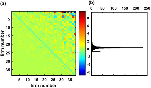
Figure 7.1. (a) Matrix I for Ttr =1000. (b) The corresponding histogram of its elements Iij (the secondary peak at −1 corresponds to the diagonal elements).
Download figure:
Standard image High-resolution imageFirst, from equation (7.5), the larger entries of Σ occur at the upper left corner (panel (a) of figure 7.2). Second, since  , the larger entries of this MaxEnt matrix will concentrate at the bottom right corner (panel (b) of figure 7.2). This can be shown by using that
  = adj(Σ)/det(Σ) (equation (vi) of Box 5.1). Thus, for firms with larger market values adj(Σ) ≪ det(Σ); conversely, for firms with smaller market values adj(Σ) ≫ det(Σ). And this explains the places where the smaller (larger) values of M do occur.

Figure 7.2. Covariance and MaxEnt interaction matrix for Ttr = 1000. (a) Covariance Σ matrix. (b)  matrix. (c) MaxEnt interaction matrix I.
Download figure:
Standard image High-resolution imageSecond, to obtain the MaxEnt interaction matrix I the entries of each row i of M are divided by Mii ; since Mii increases with i this implies that the stronger interaction coefficients will appear in the upper right corner (panel (c) of figure 7.2).
We will use the RDPME equation (7.4) to predict the market shares for Ttr + 1 ⩽ t ⩽ T = Ttr + Tv with an interaction matrix I estimated for t = Ttr. It is worth remarking that this matrix depends of the training period. Figure 7.3 shows the matrices I obtained for different training periods; in the left column Ttr = 100, 300 and 500 days, while in the right column Ttr =1000, 1200 and 1400.

Figure 7.3. Variation of I with the training period. Left column, (a): Ttr = 100, (b): Ttr = 300, (c): Ttr = 500 days. Right column, (d): Ttr = 1000, (e): Ttr = 1200, (f): Ttr = 1400 days.
Download figure:
Standard image High-resolution imageBy simple visual inspection it seems that I changes faster from lower values of Ttr. In the appendix at the end of this chapter we propose a metric to quantify the variation rate of an arbitrary matrix M, and that indicates that after Ttr = 600 the variation rate for matrix I stabilizes thus suggesting the entrance of the market into a kind of stationary state.
Growth rates
To compare predictions from the RDE against the observed xi (t) for t > Ttr, we still have to estimate the growth rate ri parameter. There are different alternative procedures to obtain this estimate from equation (7.4). One direct way is by taking:
The maximum in equation (7.6) is because the sign of xi
(t + 1) − xi
(t) in the replicator dynamics equation (7.3) must be the same as the one of  , i.e., it must be determined by whether the fitness of firm i is above or below the weighted average fitness, and thus ri
must be ⩾ 0 for all i. Therefore, for a given training period there are firms with growth rates ri
>0 and others with ri
= 0. Typically, half of the firms have ri
>0. The RDPME reduces for firms with ri
= 0 to a 'null' model which predicts that the share of company i remains constant, i.e.,
, i.e., it must be determined by whether the fitness of firm i is above or below the weighted average fitness, and thus ri
must be ⩾ 0 for all i. Therefore, for a given training period there are firms with growth rates ri
>0 and others with ri
= 0. Typically, half of the firms have ri
>0. The RDPME reduces for firms with ri
= 0 to a 'null' model which predicts that the share of company i remains constant, i.e.,  = constant = xi
(Ttr) for all t>Ttr. An alternative estimate of ri
from equation (7.4) is by using least squares, however, this method yields larger errors.
= constant = xi
(Ttr) for all t>Ttr. An alternative estimate of ri
from equation (7.4) is by using least squares, however, this method yields larger errors.
7.5. Model validation
7.5.1. Beat the market
The random walker as standard benchmark
According to the RWH, stock market prices evolve as a random walk. As we have seen, this hypothesis is consistent with the EMH, which implies that it is impossible to 'beat the market' consistently.
We have also noticed that both the RWH and the EMH have been challenged by economists and investors who claim that stock market prices may move in trends and that the market is predictable to some degree. Indeed, there have been several economic studies and tests supporting this view (Lo 1999, 2004, Fromlet 2001, Lo et al 2002).
In any case, the standard model for stock prices is the geometric Brownian motion (Ross 2014). Therefore, here we use the discrete-time version of the geometric Brownian motion, aka geometric random walk (grw), as a model to compare the RDPME. Denoting by wi the natural logarithm of the market value of company number i, it is easy to show that if it evolves as a random walk with probability pi and 'step' si , then its average at time step t will be given by

where wi (t0) is its initial value at time step t0. Then, the training period is used to estimate parameters pi and si of equation (7.7) as:
And the grw predictions of market values for t ⩽ Tv are thus obtained as:

Therefore, the corresponding shares are given by:
Quantifying the accuracy of predictions through the percentage errors of share trajectories
To compare accuracy for predicting future fractions xi of the RDPME, equation (7.4), versus the one of the grw benchmark forecasting, equation (7.10), the procedure is as follows:
First, the mean absolute percentage error (MAPE) are computed over the validation period Tv, for each firm i with the two formulas. Denoting by xpred predictions using either the RDPME or the grw, the MAPE for firm i is given by:

This metric quantifies the error of the predicted 'trajectory' for the share xi
of firm i between days Ttr + 1 and T
![$\mathit{\unicode[Book Antiqua]{x76}}$](https://content.cld.iop.org/books/10__1088_978-0-7503-3931-5/revision2/bk978-0-7503-3931-5ch7ieqn28.gif) with respect to the empirical trajectory it has followed.
with respect to the empirical trajectory it has followed.
Second, to obtain a global assessment of the accuracy of the method, the average of MAPEi over all firms is taken thus producing a global MAPE denoted as GMAPE:

The smaller this global metric the more accurate is the method as a whole.
7.5.2. Quantitative predictions for individual companies
Let us first analyze the accuracy of RDPME short-term and long-term predictions for each company. This is done by considering a relatively short validation period of T
![$\mathit{\unicode[Book Antiqua]{x76}}$](https://content.cld.iop.org/books/10__1088_978-0-7503-3931-5/revision2/bk978-0-7503-3931-5ch7ieqn30.gif) = 50 days (and for 14 training periods, Ttr = 100, 200, ..., 1300, 1400 days) and a relatively long validation period of T
= 50 days (and for 14 training periods, Ttr = 100, 200, ..., 1300, 1400 days) and a relatively long validation period of T
![$\mathit{\unicode[Book Antiqua]{x76}}$](https://content.cld.iop.org/books/10__1088_978-0-7503-3931-5/revision2/bk978-0-7503-3931-5ch7ieqn31.gif) = 500 days (and for five training periods, Ttr = 500, 600, 700, 800 and 900 days).
= 500 days (and for five training periods, Ttr = 500, 600, 700, 800 and 900 days).
Results for both validation periods T
![$\mathit{\unicode[Book Antiqua]{x76}}$](https://content.cld.iop.org/books/10__1088_978-0-7503-3931-5/revision2/bk978-0-7503-3931-5ch7ieqn32.gif) = 50 days and T
= 50 days and T
![$\mathit{\unicode[Book Antiqua]{x76}}$](https://content.cld.iop.org/books/10__1088_978-0-7503-3931-5/revision2/bk978-0-7503-3931-5ch7ieqn33.gif) = 500 days (and for the corresponding different training periods Ttr) are depicted in figure 7.4. In this figure it is also indicated for which firms the estimated ri
>0, and thus the RDPME predicts a variable share, different from the empirical share at t =
Ttr. In panels (a) and (c) if the cell at (Ttr,i) is black it means that for this company i and this training period Ttr equation (7.6) produces a positive growth rate parameter ri
. Conversely, if the cell is white it means that the obtained ri
by equation (7.6) is 0 and thus the RDPME predicts a market share of this firm
= 500 days (and for the corresponding different training periods Ttr) are depicted in figure 7.4. In this figure it is also indicated for which firms the estimated ri
>0, and thus the RDPME predicts a variable share, different from the empirical share at t =
Ttr. In panels (a) and (c) if the cell at (Ttr,i) is black it means that for this company i and this training period Ttr equation (7.6) produces a positive growth rate parameter ri
. Conversely, if the cell is white it means that the obtained ri
by equation (7.6) is 0 and thus the RDPME predicts a market share of this firm  = constant = xi
(Ttr) for all t>Ttr. Indeed, roughly half of the cells in panels (a) and (c) are black, meaning that the growth rate parameter ri
produced by equation (7.6) is positive 50% of the times. For example, notice that there are two companies for which ri
>0 for all training periods: MSFT (company #2) and WMT (company #8). Additionally, there is one firm, MCK (company #34), such that ri
= 0 for all training periods. Colored cells in panels (b) and (d) denote the MAPE for cell (Ttr,i) given by equation (7.11). Blue (red) indicates small (large) MAPE. A pattern which can be observed by direct inspection is that larger MAPE occurs for smaller cap firms. This pattern is particularly evident for T
= constant = xi
(Ttr) for all t>Ttr. Indeed, roughly half of the cells in panels (a) and (c) are black, meaning that the growth rate parameter ri
produced by equation (7.6) is positive 50% of the times. For example, notice that there are two companies for which ri
>0 for all training periods: MSFT (company #2) and WMT (company #8). Additionally, there is one firm, MCK (company #34), such that ri
= 0 for all training periods. Colored cells in panels (b) and (d) denote the MAPE for cell (Ttr,i) given by equation (7.11). Blue (red) indicates small (large) MAPE. A pattern which can be observed by direct inspection is that larger MAPE occurs for smaller cap firms. This pattern is particularly evident for T
![$\mathit{\unicode[Book Antiqua]{x76}}$](https://content.cld.iop.org/books/10__1088_978-0-7503-3931-5/revision2/bk978-0-7503-3931-5ch7ieqn35.gif) = 500 days, where the orange-red cells occur mostly in the lower part of panel (d).
= 500 days, where the orange-red cells occur mostly in the lower part of panel (d).
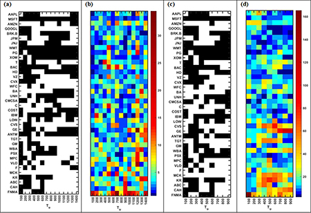
Figure 7.4. The suitability of RDPME and the accuracy of its predictions for each firm. (a) and (b): validation period T
![$\mathit{\unicode[Book Antiqua]{x76}}$](https://content.cld.iop.org/books/10__1088_978-0-7503-3931-5/revision2/bk978-0-7503-3931-5ch7ieqn2.gif) = 50 days, training period Ttr+T
= 50 days, training period Ttr+T
![$\mathit{\unicode[Book Antiqua]{x76}}$](https://content.cld.iop.org/books/10__1088_978-0-7503-3931-5/revision2/bk978-0-7503-3931-5ch7ieqn3.gif) = 100, 200,...,1400. (c) and (d): validation period T
= 100, 200,...,1400. (c) and (d): validation period T
![$\mathit{\unicode[Book Antiqua]{x76}}$](https://content.cld.iop.org/books/10__1088_978-0-7503-3931-5/revision2/bk978-0-7503-3931-5ch7ieqn4.gif) = 500 days, training period Ttr+T
= 500 days, training period Ttr+T
![$\mathit{\unicode[Book Antiqua]{x76}}$](https://content.cld.iop.org/books/10__1088_978-0-7503-3931-5/revision2/bk978-0-7503-3931-5ch7ieqn5.gif) = 100, 200,...,900. In panels (a) and (c) a black cell at (Ttr,i) means that for this company i and this training period Ttr the obtained growth rate parameter ri
—through equation (7.6)—is positive. Conversely, a white cell means that for this company i and this training period Ttr the obtained ri
is equal to 0 and thus the RDPME method reduces to the null model, i.e.,
= 100, 200,...,900. In panels (a) and (c) a black cell at (Ttr,i) means that for this company i and this training period Ttr the obtained growth rate parameter ri
—through equation (7.6)—is positive. Conversely, a white cell means that for this company i and this training period Ttr the obtained ri
is equal to 0 and thus the RDPME method reduces to the null model, i.e.,  = constant = xi
(Ttr) for all t>Ttr. Colored cells in panels (b) and (d) denote the corresponding MAPE for each cell (Ttr,i) (equation (7.11)). Blue (red) indicates small (large) MAPE.
= constant = xi
(Ttr) for all t>Ttr. Colored cells in panels (b) and (d) denote the corresponding MAPE for each cell (Ttr,i) (equation (7.11)). Blue (red) indicates small (large) MAPE.
Download figure:
Standard image High-resolution imageRegarding forecasting trajectories of shares of companies x(t), figure 7.5 shows the empirical trajectories for the shares of 20 companies (in black) and those predicted by RDPME, equation (7.4) (red), and grw, equation (7.11) (blue), for Ttr = 200 and Tv = 50 days. The 20 companies are those such that equation (7.7) produces, for Ttr = 200 days, an intrinsic growth rate ri
>0 and thus equation (7.4) leads to a share xi
that varies with time. For the other 18 firms equation (7.7) produces an intrinsic growth rate ri
= 0 and thus the prediction of RDPME through equation (7.4) is a horizontal line xpred(t) = xi
(200) for all t such that 200 <t⩽ T
![$\mathit{\unicode[Book Antiqua]{x76}}$](https://content.cld.iop.org/books/10__1088_978-0-7503-3931-5/revision2/bk978-0-7503-3931-5ch7ieqn36.gif) = 50 days (not shown in the figure). Notice that while empirical shares describe wiggled curves, those predicted by RDPME or grw do not. This difference is because the RD is a deterministic equation and the grw predictions are mean values of a stochastic process (which yields also deterministic results).
= 50 days (not shown in the figure). Notice that while empirical shares describe wiggled curves, those predicted by RDPME or grw do not. This difference is because the RD is a deterministic equation and the grw predictions are mean values of a stochastic process (which yields also deterministic results).
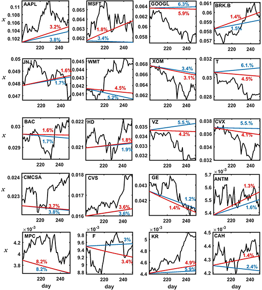
Figure 7.5. Shares for the 20 firms such that for Ttr = 200 the estimated growth rate ri
> 0 along T
![$\mathit{\unicode[Book Antiqua]{x76}}$](https://content.cld.iop.org/books/10__1088_978-0-7503-3931-5/revision2/bk978-0-7503-3931-5ch7ieqn7.gif) = 50 days. Empirical values (black), grw predictions (blue) and RDPME predictions (red). Percentages in each panel denote the MAPE for grw (blue) and RDPME predictions (red).
= 50 days. Empirical values (black), grw predictions (blue) and RDPME predictions (red). Percentages in each panel denote the MAPE for grw (blue) and RDPME predictions (red).
Download figure:
Standard image High-resolution imageAs we can see from figure 7.5, for this particular partition of Ttr = 200 and Ttr = 50, the RDPME model outperforms the grw benchmark (i.e., it achieves a smaller MAPE) for 16 out of 20 = 80% of these companies, it underperforms the grw for 2 in 20 = 10% and both tie for 2 in 20 = 10%. When considering all the 38 companies, including those with ri = 0, these percentages become: 63%, 26% and 11%.
Figure 7.6 is the same as figure 7.5 but for a much longer training period; Ttr = 700 days. In this case there are 16 such that equation (7.7) produces an intrinsic growth rate ri >0 and thus equation (7.4) leads to a share xi that varies with time.

Figure 7.6. Shares for the 16 firms for which, when Ttr = 700, the estimated intrinsic growth rate ri
>0 and thus RDPME predicts a variable share for those companies along ![${T}_{\mathit{\unicode[Book Antiqua]{x76}}}$](https://content.cld.iop.org/books/10__1088_978-0-7503-3931-5/revision2/bk978-0-7503-3931-5ch7ieqn8.gif) = 700 days. Empirical values (black), grw predictions (blue) and RDPME predictions (red). Percentage in each panel denote the corresponding MAPE for grw predictions (blue) and RDPME predictions (red).
= 700 days. Empirical values (black), grw predictions (blue) and RDPME predictions (red). Percentage in each panel denote the corresponding MAPE for grw predictions (blue) and RDPME predictions (red).
Download figure:
Standard image High-resolution imageNow the RDPME model outperforms the grw benchmark for 10 out of 16 = 63% of the companies; these companies are MSFT, BRK.B, WMT, HD, UNH, CMSA, COST, IBM, LOW and PSX. When considering all the 38 companies, including those with ri = 0, the percentage of wins becomes 53%. For the great majority of partitions of Ttr−Ttr, these percentages are qualitatively similar.
It is worth remarking that the MAPEs of both methods for this larger validation period are in general much larger ( = 26.1%,
  = 28.1%). This increase in the errors is an expected result, we have to take into account that the validation period in this latter case comprises more than two years of trade.
7.5.3. Global accuracy of the RDPME method
Table 7.2 shows the GMAPE, both for the RDPME and grw, for different partitions of Ttr and Tv (in days).
Table 7.2. GMAPE, i.e., mean absolute percentage errors (MAPE) averaged over firms produced by the Replicator Dynamics equation (RDPME) equation (7.11) compared with the geometric random walk (grw) equation (7.10) for different training and validation periods (fixed initial time day = 1). The last column corresponds to % of times the RDPME leads to a smaller relative error than the grw. Numbers in bold correspond to minimum GMAPE for a given validation period.
| Validation period (days) ↓ | Method | Training period (days) → | % of wins | ||||||||||||
| 100 | 200 | 300 | 400 | 500 | 600 | 700 | 800 | 900 | 1000 | 1100 | 1200 | 1300 | |||
| 100 | RDMPE | 6.2 | 6.6 | 5.4 | 6.4 | 8.8 | 5.0 | 7.4 | 5.7 | 6.5 | 7.8 | 6.4 | 8.8 | 7.5 | 76.9 |
| grw | 6.5 | 7.2 | 5.4 | 6.8 | 9.2 | 5.7 | 7.9 | 5.6 | 7.0 | 6.9 | 6.7 | 9.6 | 7.6 | 23.1 | |
| 200 | RDMPE | 11.4 | 9.0 | 9.2 | 10.4 | 11.7 | 8.3 | 9.8 | 9.0 | 11.0 | 11.2 | 10.1 | 10.8 | 83.3 | |
| grw | 13.3 | 10.0 | 8.8 | 11.1 | 13.5 | 9.9 | 10.6 | 9.5 | 10.2 | 9.4 | 10.9 | 11.9 | 16.7 | ||
| 300 | RDMPE | 13.6 | 10.9 | 12.9 | 13.1 | 13.9 | 11.5 | 13.0 | 13.3 | 15.3 | 13.0 | 12.8 | 63.6 | ||
| grw | 18.5 | 12.0 | 12.3 | 15.0 | 16.7 | 13.9 | 14.4 | 12.9 | 13.6 | 11.6 | 13.6 | 36.4 | |||
| 400 | RDMPE | 15.6 | 12.4 | 16.1 | 15.0 | 16.3 | 15.1 | 16.8 | 17.8 | 17.8 | 14.5 | 60 | |||
| grw | 23.6 | 13.3 | 16.1 | 18.2 | 20.4 | 18.4 | 18.0 | 16.7 | 16.2 | 13.9 | 40 | ||||
| 500 | RDMPE | 17.5 | 13.5 | 19.1 | 16.7 | 19.4 | 18.6 | 20.7 | 20.8 | 19.8 | 77.8 | ||||
| grw | 30.0 | 14.4 | 19.4 | 21.6 | 25.0 | 22.9 | 21.8 | 19.9 | 18.8 | 22.2 | |||||
| 600 | RDMPE | 19.0 | 14.8 | 22.2 | 19.1 | 22.5 | 22.2 | 23.6 | 23.3 | 87.5 | |||||
| grw | 36.6 | 15.7 | 22.7 | 25.8 | 29.6 | 27.4 | 25.0 | 23.1 | 12.5 | ||||||
| 700 | RDMPE | 20.2 | 16.4 | 25.7 | 21.6 | 25.8 | 25.0 | 26.1 | 100 | ||||||
| grw | 41.9 | 17.4 | 26.4 | 30.1 | 34.6 | 31.6 | 28.1 | 0 | |||||||
| % of wins RDEMPE | 100 | 100 | 57.1 | 100 | 100 | 100 | 100 | 16.7 | 16.7 | 0 | 100 | 100 | 100 | ||
RDPME: replicator dynamics, grw: geometric random walk
Remarks:
- i.For the great majority of partitions the RDPME yields a smaller GMAPE than the grw.
- ii.For each training period the RDPME achieves always the minimum GMAPE.
- iii.Most of the minimum GMAPE correspond to Ttr = 200, thus suggesting a sort of trade-off implying that very large training periods do not provide larger accuracy.
- iv.As expected, for a given training period, the GMAPE grows with the validation period (i.e., the larger the forecast horizon the less accurate the predictions).
7.6. Conclusion: balance, caveats, extensions and improvements
Natural selection in biology rests on a rigorous explanatory power, including quantitative checkable predictions. For example, we have seen in chapter 4 how a simple modelling is able to reproduce the observed frequency variations of COVID-19 variants. On the other hand, its economic counterpart is often an example of the truism that surviving firms are efficient because only the efficient survive (Knudsen 2002). In particular, the model of RD provides important insights in the evolution of markets but has not met with much empirical support (Cantner et al 2019).
Here we attempted to fill that gap by providing quantitative testable predictions that hopefully will contribute toward making the replicator dynamics more than just a theoretically elegant model but also a relevant economic quantitative tool regarding empirical data. With this aim we resorted to the maximum entropy principle, a fruitful approach used in several different fields to make least biased inferences with incomplete information, to infer from empirical financial time series the payoff matrix of the RD equation.
The main finding was that the resulting RDPME method outperforms the neutral benchmark of the geometric random walk (grw) in predicting future shares xi for most of the companies and for most of the partitions in training and validation periods. It is worth mentioning that the relative errors of the RDPME are in general only modestly smaller than those produced by the grw. Hence, perhaps this is a sign that financial markets need to be explained in terms of truly complex systems modelling (Kuhlmann 2014).
Let us conclude this chapter by reviewing some caveats, extensions and possible future improvements. A general intrinsic limitation of the RD as a forecasting tool for stock prices is that it works with shares or frequencies as variables so it can predict market shares rather than market caps or the price of a stock. One way to overcome this drawback is by introducing an additional variable M for the total market value of the market (i.e., the sum of all market caps of the S firms considered). This variable is shown in figure 7.7 and exhibits a clear growing trend. Therefore we can fit the trajectory of M(t) for a given Ttr using least squares and obtain a predicted total cap for the validation period Tv. Again, how to do this is not trivial and involves a sort of handy craft. If for example we choose Ttr = 1000 days, the least squares prediction (blue line) clearly underestimates the total market cap for t = 1001,...,1455 days. Surprisingly, a substantially better prediction for the latter part of the time series is achieved for this system using a much shorter Ttr = 200 days (red line).

Figure 7.7. Time evolution of the aggregated market cap of the 38 companies M(t) along the considered period of 1455 days. Empirical values (black) and RDPME predictions (dashed lines) through linear regression, computed from the first Ttr days, for the remaining ![${T}_{\mathit{\unicode[Book Antiqua]{x76}}}$](https://content.cld.iop.org/books/10__1088_978-0-7503-3931-5/revision2/bk978-0-7503-3931-5ch7ieqn9.gif) = 1455−Ttr days; for Ttr = 1000 (blue) and Ttr = 200 days (red).
= 1455−Ttr days; for Ttr = 1000 (blue) and Ttr = 200 days (red).
Download figure:
Standard image High-resolution imageAnother limitation of the RD equation in describing the evolution of competing phenotypes is that it does not incorporate mutation and so is not able to innovate new types of phenotypes. To overcome such a drawback the RD equation is usually extended to the replicator–mutator (RM) equation (Nowak 2006), i.e., the RD equation with mutations. With the introduction of changes by random mutations of the set of phenotypes it includes a source of innovation lacking in the RD. The RM would allow one to model changes in the list of top firms (actually this list usually changes from one year to the next).
There is also a caveat regarding the set of selected firms: they are the largest (in revenues) US listed companies in the NYSE. But there are also some non-US companies operating in the US with larger revenues than some of the companies in this set. We used this criterion of US based firms to select the 'community' because it seemed more clear cut and due to the global dominance of US companies (Ross 2020).
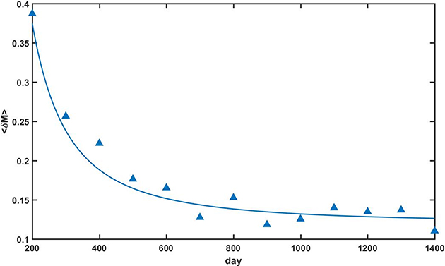
Appendix A: A metric to measure the pace of change of the payoff matrix
As mentioned, the I matrix changes with the training period. From simple visual inspection it seems that I changes faster from lower values of Ttr. In the appendix at the end of this chapter we propose a metric. Therefore, it is important to measure the variation rate of M because the faster the pace the shorter the validation period. With this aim we introduced the following metric for comparing differences between the non-diagonal parts of M at two times, t and t': 5
where we denoted by the angle brackets 〈〉 averages over all (S−1)×(S−1) non-diagonal matrix elements. We take the absolute value of variations of each matrix element to avoid cancellations when performing these averages.
Figure A.1 shows the variation of δM (Ttr ,Ttr + 100), given by equation (A.1), versus the time t measured in days. That is, the first point corresponds to the difference between a training period Ttr = 100 and a time t = Ttr + 100 = 200, the second point corresponds to the difference between a training period Ttr = 200 and a time t = Ttr + 100 = 300, and so on. Notice that δM (Ttr , Ttr +100) first decreases quickly and then after Ttr = 600 seems to stabilize to a value around 0.12.
Figure A.1. Variation with time (measured in days) of M, for intervals of 100 days and training periods of 100, 200, ...,1300 days (triangles) and the corresponding fit (filled curve).
Download figure:
Standard image High-resolution image
References
- Astley W G and Fombrun C J 1983 Collective strategy: social ecology of organizational environments Acad. Manage. Rev. 8 576–87
- Bachelier L 1900 Théorie de la spéculation Ann. Sci. Ec. Norm. Super. 17 21–86
- Boyte-White C 2020 Market capitalization versus market value: what's the difference? Investopedia https://investopedia.com/ask/answers/122314/what-difference-between-market-capitalization-and-market-value.asp accessed 11 January 2022
- Cantner U, Savin I and Vannuccini S 2019 Replicator dynamics in value chains: explaining some puzzles of market selection Ind. Corp. Change 28 589–611
- Cantner U 2017 Structural change in heterogeneous actor populations Foundations of Economic Change: A Schumpeterian View on Behaviour, Interaction and Aggregate Outcomes , ed A Pyka and U Cantner (Berlin: Springer)
- Case J 2008 Competition: The Birth of a New Science (New York: Hill and Wang)
- Chan L K C, Karceski J J and Lakonishok J 1999 On Portfolio Optimization: Forecasting Covariances and Choosing the Risk Model NBER Working paper No. w7039, Available at SSRN:https://ssrn.com/abstract=156690
- Chen M J 2002 Transcending paradox: the Chinese 'middle way' perspective Asian-Pac. J. Manage. 19 179–99
- Clarke-Hill C, Li H and Davies B 2003 The paradox of co-operation and competition in strategic alliances: towards a multi-paradigm approach Manage. Res. News 26 1–20
- Cootner P H 1964 The Random Character of Stock Market Prices (Cambridge, MA: MIT Press)
- Czakon W 2010 Emerging coopetition: an empirical investigation of coopetition as inter-organizational relationship instability Coopetition. Winning Strategies for the 21st Century , ed S Yami, S Castaldo, G Dagnino and F Le Roy (Cheltenham: Edward Elgar Publishing) pp 58–73
- Dhir R 2021 Efficient market hypothesis: is the stock market efficient? Investopedia https://investopedia.com/articles/basics/04/022004.asp accessed 11 October 2021
- Dosi G and Nelson R R 1994 An introduction to evolutionary theories in economics J. Evol. Econ 4 153–72
- Downey L 2021 Efficient market hypothesis (EMH) Investopedia https://investopedia.com/terms/e/efficientmarkethypothesis.asp accessed 4 October 2021
- Dyer J and Singh H 1998 The relational view: cooperative strategy and sources of interorganizational competitive advantage Acad. Manage. Rev. 24 660–79
- Einstein A 1905 Über die von der molekularkinetischen Theorie der Wärme geforderte Bewegung von in ruhenden Flüssigkeiten suspendierten Teilchen' [On the movement of small particles suspended in stationary liquids required by the molecular-kinetic theory of heat] Ann. Phys. 322 549–60
- Emary C and Fort H 2021 Markets as ecological networks: inferring interactions and identifying communities J. Complex Netw. 9 1–17
- Engle R F 2009 Anticipating Correlations: A New Paradigm for Risk Management (Princeton, NJ: Princeton University Press)
- Fama E F 1965 Random walks in stock market prices Financ. Anal. J. 21 55–9
- Fama E F 1970 Efficient capital markets: a review of theory and empirical work J. Finance 25 383
- Fortune 2018 https://fortune.com/fortune500/2018/
- Fortune 2019 https://fortune.com/fortune500/2019/
- Fromlet H 2001 Behavioral finance—theory and practical application Bus. Econ. 36 63–9
- Knudsen T 2002 Economic selection theory J. Evol. Econ. 12 443–70
- Kuhlmann M 2014 Explaining financial markets in terms of complex systems Phil. Sci. 81 1117–30
- Lakka S, Michalakelis C, Varoutas D A and Martakos D 2013 Competitive dynamics in the operating systems market: modeling and policy implications Technol. Forecast. Soc. Change 80 88–105
- Liberto D 2021 Adaptive market hypothesis (AMH) Investopedia https://investopedia.com/terms/a/adaptive-market-hypothesis.asp accessed 4 October 2021
- Lo A 1999 A Non-Random Walk Down Wall Street (Princeton, NJ: Princeton University Press)
- Lo A, Mackinlay W and Craig A 2002 A Non-Random Walk Down Wall Street 5th edn (Princeton, NJ: Princeton University Press) pp 4–47
- Lo A W 2004 The efficient market hypothesis: market efficiency from an evolutionary perspective J. Portfolio Manage. 30 15–29
- Malkiel B G 1973 A Random Walk Down Wall Street 6th edn (New York: W.W. Norton & Company, Inc.)
- Mazzucato M 2000 Firm Size, Innovation, and Market Structure: The Evolution of Industry Concentration and Instability (Cheltenham: Edward Elgar Publishing)
- Moore J F 1993a Predators and prey: a new ecology of competition Harvard Business Review May/June 1993
- Moore J F 1993b The Death of Competition: Leadership and Strategy in the Age of Business Ecosystems (New York: Harper Paperbacks)
- Morningstar 2019 Morningstar's Active/Passive Barometer August 2019
- Nelson R R and Winter S G 1982 An Evolutionary Theory of Economic Change (Cambridge, MA: Harvard University Press)
- Nowak M A 2006 Evolutionary Dynamics: Exploring the Equations of Life (Cambridge, MA: Belknap Press) pp 272–73
- 2021 NYSE https://nyse.com/market-cap accessed 17 September 2021
- Oliver A L and Ebers M 1998 Networking network studies: an analysis of conceptual configurations in the study of inter-organizational relationships Organ. Stud. 19 549–83
- Pearson K 1905 The problem of the random walk Nature 72 294–342
- 2020 Pfizer and Biontech Announce Further Details on Collaboration to Accelerate Global Covid-19 Vaccine Development Pfizer https://investors.pfizer.com/investor-news/press-release-details/2020/Pfizer-and-BioNTech-Announce-Further-Details-on-Collaboration-to-Accelerate-Global-COVID-19-Vaccine-Development/default.aspx accessed 18 June 2021
- 2021 Pfizer and BioNTech to Provide 500 Million Doses of COVID-19 Vaccine to U.S. Government for Donation to Poorest Nations Pfizer https://pfizer.com/news/press-release/press-release-detail/pfizer-and-biontech-provide-500-million-doses-covid-19 accessed 18 June 2021
- Porter M E 1980 Competitive Strategy (New York: Free Press)
- Protos 2021 Crypto Trading Hamster Outperforms Bitcoin, Warren Buffett, Cathie Wood https://protos.com/crypto-trading-hamster-goxx-outperforms-bitcoin-buffett-wood/
- Quandl 2019 Core US Fundamentals Dataset Available at http://www.quandl.com/databases/SF1
- Rayleigh L 1905 The problem of the random walk Nature 72 318
- Regnault J 1863 Calcul des Chances et Philosophie de la Bourse (London: Forgotten Books) Classic Reprint Series, 4 March 2018
- Ross S M 2014 Variations on Brownian motion Introduction to Probability Models 11th edn (Amsterdam: Elsevier) pp 612–14
- Ross J 2020 The Dominance of U.S. Companies in Global Markets https://visualcapitalist.com/us-companies-global-markets/ accessed 18 November 2021
- Rumelt R P 1991 How much does industry matter? Strateg. Manage. J. 12 167–85
- Samuelson P 1965a Rational theory of warrant pricing Ind. Manage. Rev. 6 13–39
- Samuelson P 1965b Proof that properly anticipated prices fluctuate randomly Ind. Manage. Rev. 6 41–9
- Shmueli G and Lichtendahl K C 2016 Practical Time Series Forecasting with R: A Hands-on Guide 2nd edn (Green Cove Springs, FL: Axelrod Schnall Publishers)
- Toynbee A J 1946 A Study of History, Vol. 1: Abridgement of Volumes I–VI New Edition 1999 (Oxford: Oxford University Press)
- Vasicek O A and McQuown J A 1972 The efficient market model Financ. Anal. J. 28 71–84
- Yami S 2010 Introduction—coopetition strategies: towards a new form of inter-organizational dynamics? Coopetition. Winning Strategies for the 21st Century , ed S Yami, S Castaldo, G Dagnino and F Le Roy et al (Cheltenham: Edward Elgar Publishing) pp 58–73
Footnotes
- 1
- 2
Thus, for example a firm like Dell Technologies, ranked 35 in the 2018 Fortune 500 list (Fortune 2018), wasn't included because from 2014 to 2016 it wasn't in the Fortune 500 list.
- 3
Throughout this chapter we will use indistinctly 'market value' and 'market capitalization' or 'market cap' for short. Market capitalization is basically the number of a company's shares outstanding multiplied by the current price of a single share. More rigorously speaking, market value is more amorphous and more complicated, assessed using numerous metrics and multiples, such as price-to-earnings, price-to-sales, and return-on-equity (Boyte-White 2020).
- 4
- 5
Alternatively, the Euclidean norm can be used. I checked it produces similar results although they are less clear-cut.