
Topological features
Published November 2018
•
Copyright © IOP Publishing Ltd 2018
Pages 2-1 to 2-37
You need an eReader or compatible software to experience the benefits of the ePub3 file format.
Download complete PDF book, the ePub book or the Kindle book

Permissions
Abstract
The structure of an optical vortex is described in this chapter. The shape of the wavefront, the amplitude and phase variation in the vortex beam are presented. Phase contours and the real/imaginary zero curves of complex fields are useful in the study of topological features. The difference between phase contour, curves of zeros and bifurcation lines is made clear. Similarly, the difference between the charge, index and order of a vortex is presented. The critical points such as extrema, saddles, vortices and their occurrence in optical fields are introduced. The governing rules on critical point disintegration under perturbation are presented. Different sign rules and conservation rules are presented. Vortex trajectories in three dimensions and rules pertaining to the allowed trajectories are discussed with the help of manifolds. Finally, different types of singularities are listed.
2.1. Introduction
To understand many of the properties in the phase distribution, knowledge of the shape of the wavefront and the topological features are important. Many of the beam characteristics such as propagation, divergence, and diffraction are dependent on the wavefront. Critical points shape up the wavefront and hence this chapter starts with the study of wavefronts.
The structure of an optical vortex wavefront, phase and amplitude distributions are studied. In field distributions, phase contours, real and imaginary zero curves are employed in the discussion on the topological features of the phase singularity. Other critical points such as extrema and saddles in fields and their coexistence with vortices are described. Critical points can also undergo disintegration and there can be byproducts. The critical points can be analyzed with the help of phase contours. The difference between phase contour, zeros of real/imaginary part of the field and bifurcation lines are made clear. Similarly there is also difference between the charge, index and order of a vortex. There are different sign rules and conservation rules for vortices in distributions. With the help of Berry's paradox, it is shown that concepts like charge and its conservation can be dispensed with and instead vortex trajectories can be used. To deal with these vortex trajectories, concepts like topological manifolds are used.
2.2. Wavefront shape
The phase contour surfaces of an optical field are the wavefronts. The wavefronts are usually drawn with a spacing of λ between two consecutive surfaces. Depending on the shape of the wavefronts, the waves are named as plane, spherical or cylindrical waves. From a primary wavefront, according to Huygen's principle, the secondary wavelets lead to the construction of the next wavefront. The next wavefront, that is constructed is also of the same type, i.e. a plane wavefront leads to the construction of plane wavefront and so on.
For a phase singular beam, the wavefronts have a helical shape [1–4] and are shown in figure 2.1. It is a ramp-like
structure winding about the phase singular point which draws a curve in three
dimensions, upon propagation. Depending on the handedness of the phase ramp, the
singularity is termed as positive (anti-clockwise ramp) or negative (clockwise ramp) as
shown in figure 2.2. Along
the general propagation direction the distance between two consecutive constant phase
surfaces is λ. But there is a little twist in the story. Due to the
presence of the phase singularity the adjacent wavefronts get connected and there is a
single wavefront spanning the entire space and the notion of distance between two
wavefronts becomes meaningless. When a wavefront has a vortex, the wavefront extends
from  to
to  along the propagation direction. Also construction from one wavefront
to another becomes difficult to comprehend as there is going to be only one
wavefront.
along the propagation direction. Also construction from one wavefront
to another becomes difficult to comprehend as there is going to be only one
wavefront.

Figure 2.1. Phase distributions and the wavefront structures corresponding to (a) plane wave
with a tilt, (b) spherical wave and (c) helical wave of charge +1. On the wavefront
the phase is constant and hence if the observation plane is of the same shape as
that of the wavefront, the phase distribution would have been constant. But normally
phase distribution is the one observed on a plane surface (say  plane if the nominal propagation direction is along
z).
plane if the nominal propagation direction is along
z).
Download figure:
Standard image High-resolution image
Figure 2.2. Phase distribution and wavefront shape of (a) a positive and (b) a negative vortex.
Download figure:
Standard image High-resolution imageImagine that travel on a circular path is performed over the wavefront surface. In a plane wave or in a spherical wave, travel between two consecutive wavefront surfaces entails a jump λ while such a jump is not needed if the travel is carried over a helical wavefront. When multiple spatially distributed singularities are present these ramps allow forward and backward travel from one wavefront to succeeding or preceding wavefronts while maintaining the sense of (say, clockwise) direction of the travel path. To be exact, I cannot use the term different wavefronts—hence the travel results in forward and backward displacements on the same surface which is cut and stitched at various places to the preceding or succeeding wavefronts. (This can be seen later in this chapter where oriented curves are introduced for vortices. The propagation vector spirals around the vortex core and this indicates that backward flow of energy is possible.) For a vortex of higher charge, in the wavefront there are multi-start ramps starting from one surface leading to the next surface at a height of λ, as depicted in figure 2.3. This is similar to going from one floor to the next floor in a building using (multiple start ramps) any one of the many helical ramps. For example for a topological charge of 2, there are two ramps starting simultaneously from one floor and leading to the next floor and one can use either one of them to go from one floor to the other.

Figure 2.3. Vortices of higher charges and different polarities. Phase and wavefront maps.
Download figure:
Standard image High-resolution imageInstead of discussing travel from one surface to another let us consider travel over a
closed path on the wavefront. For a non-singular beam, a circular closed travel path
will leave a person on the same floor (same starting point) whereas a similar circular
travel path on a singular beam around the singularity leads to climbing up/down by a
height of λ. For a vortex of charge l the height
gained is  . When there are two vortices of opposite charges present, the
evolution of the wavefront is hard to visualize as the structure continuously evolves as
depicted in figure 2.4.
There is global change in the shape of the wavefront as it propagates and is periodic.
Individually, each of the vortices has a helical structure winding in the opposite sense
to each other as the wave propagates. This can be seen by tracking the immediate
neighborhood of each vortex.
. When there are two vortices of opposite charges present, the
evolution of the wavefront is hard to visualize as the structure continuously evolves as
depicted in figure 2.4.
There is global change in the shape of the wavefront as it propagates and is periodic.
Individually, each of the vortices has a helical structure winding in the opposite sense
to each other as the wave propagates. This can be seen by tracking the immediate
neighborhood of each vortex.

Figure 2.4. Vortex dipole and the wavefront structure (a) where the 2π virtual phase jump line is pointing away from the center of the dipole, (b) where the 2π virtual phase jump is between the charges and (c) at an intermediate state. This 2π jump is called 'virtual' as at this position the wavefront is connected to the next wavefront and hence there is actually no phase jump and the wavefront is continuous. The wavefront structure from (a) to (c) can evolve by constant phase shifts.
Download figure:
Standard image High-resolution image2.3. Amplitude and phase distribution of an optical vortex beam
Now, instead of dealing with constant phase surfaces, let us examine the situation on a plane surface. For a wave traveling along the z direction, the plane under consideration is an xy-plane. The phase at each point on this plane is given by the phase distribution. The phase distributions for a spherical wave, a plane wave traveling at an angle to the z axis, and a helical wave are presented in figure 2.1.
For a non-singular beam such as a plane wave or a spherical wave, the phase distribution is such that the accumulated phase (or the phase difference between any two different spatial points) is given by

where dl is the path of integration. In equation (2.1) the phase
difference is independent of the path taken for computation. Further for closed path  . But for phase singular beams

This means  and in the neighborhood region of the singularity the gradient field
has non-zero curl or circulating phase gradient. At the point at which the singularity
is located, the phase is indeterminate. For a complex field which is single valued, at
every point the amplitude and phase take a single value and this undefined phase is
possible only by considering the amplitude to be zero at the singular point. It is also
true that at all points where the amplitude is zero, the phase is indeterminate, because
the phase is given by the ratio of the imaginary to the real part of the complex field.
The field is
and in the neighborhood region of the singularity the gradient field
has non-zero curl or circulating phase gradient. At the point at which the singularity
is located, the phase is indeterminate. For a complex field which is single valued, at
every point the amplitude and phase take a single value and this undefined phase is
possible only by considering the amplitude to be zero at the singular point. It is also
true that at all points where the amplitude is zero, the phase is indeterminate, because
the phase is given by the ratio of the imaginary to the real part of the complex field.
The field is  . At a null amplitude we have,

But an amplitude zero point does not guarantee the presence of an optical vortex at that point. For example, the Newton's ring experiment in which concentric circular interference fringes are formed due to interference of a plane and a spherical wave. The center of the fringe pattern observed in reflection is an amplitude zero point, and this happens to be an extremum point in phase but not a vortex point. Even though amplitude null makes the phase indeterminate, that point does not correspond to a wavefront with helical shape. Hence amplitude zero is a necessary condition but not sufficient condition for the existence of phase singularity. The condition given by the closed path integral equation (2.2) has to be satisfied for a vortex.
The amplitude and phase distributions of an optical vortex beam are such that at the
phase singular point the phase is undefined and the amplitude is zero. Even if you start
with a uniform background amplitude wave with an embedded vortex in it, (this is
possible by illuminating the vortex phase plate by a uniform amplitude plane wave),
during propagation at the vortex point the amplitude becomes zero due to diffraction
effects. The amplitude background can be of any form but has zero value at the vortex
point. For example, a Gaussian wave has non-zero amplitude at the center, but the
Gaussian amplitude is modulated (multiplied) with Laguerre polynomials of any order
along with an r term, resulting in the zero amplitude at the vortex
point at r = 0. Laguerre–Gaussian beams are often encountered in
singular optics. Similarly the amplitude of the vortex beam can have tan hyperbolic
variation and in that case the beam can be termed as tanh vortex. Another
kind of vortex often used in discussions is the r-vortex in which case, the
amplitude is linearly varying as a function of r. The linear increase
in amplitude as we go radially away from the origin (vortex point) leads to larger
amplitude and since the wave function is finite, this is not a physically feasible form
of describing the vortex. To avoid this amplitude blow-up a Gaussian envelope can be
used. Nevertheless use of such an r-type vortex is common and is very
helpful in understanding many of the properties of the vortex [5]. It is useful to introduce the following
way of writing the complex field for a vortex. For a positive vortex at the origin, the
field is given by (x + iy) in which the amplitude is  and the phase is arctan
  . This is in fact an r-type vortex. A negative vortex
has the complex field given by (x−iy), a vortex of
higher charge l is given by (x ± iy)l
and a vortex located at a point other than the origin is given by
(x−x0) ± i
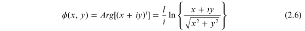
(y−y0) where (x0, y0) is the location of the phase singularity. Consider the complex function
given by
. This is in fact an r-type vortex. A negative vortex
has the complex field given by (x−iy), a vortex of
higher charge l is given by (x ± iy)l
and a vortex located at a point other than the origin is given by
(x−x0) ± i
(y−y0) where (x0, y0) is the location of the phase singularity. Consider the complex function
given by

Here the charge of the vortex is l. R and I indicate the real and imaginary parts of the complex field respectively. By denoting the zero of the real part of the field as ZR and zero of the imaginary part of the field as ZI we will discuss various aspects of the complex field in the following sections.
2.4. Topological charge
The topological charge of a phase singularity is defined by

where l is called the topological charge of the phase singularity. It can take positive and negative integer values [6, 7]. The sign of the vortex is decided by the sign of the azimuthal phase gradient. For a positive vortex, the phase increases in an anti-clockwise sense around the singular point and for a negative vortex, the phase increase is in the clockwise sense.
There are also vortices with fractional charges and they are called fractional vortices. They do not produce a donut intensity profile, but produce a radial cut in the donut shape.
2.5. Phase contours and zero crossings
Phase contours in two-dimensional phase distributions are the curves on which the phase
value is constant. Phase contours for a single vortex and a vortex diplole are shown in
figure 2.5. The random
field has a large number of vortices. The phase, phase contours and real and imaginary
zero curves for a random field are shown in figure 2.6. Contours corresponding to all phase
values terminate on the vortex giving it a star-like appearance. This is similar to
electric field lines terminating or originating from an electric charge [5]. Because of the similar
structure, the phrase 'charge' is chosen to describe the strength of the vortices.
Consider four phase contours at phase values of  and
and  that terminate on a vortex point. Phase values of zero and
π correspond to zero of the imaginary part (ZI
) of the wave function and the phase values of
that terminate on a vortex point. Phase values of zero and
π correspond to zero of the imaginary part (ZI
) of the wave function and the phase values of  and
and  correspond to zero of the real part (ZR
) of the wave function. Termination of phase contours can be seen as the zeros of
the real and imaginary part of the wave function crossing at the vortex point. A phase
contour at phase value zero and a phase contour at phase value π
terminating on a vortex point is seen as an imaginary zero curve which is continuously
passing through the vortex point. Hence by using the continuous curves of
ZI
and ZR
we can analyze the critical points. The distinction between the phase contours
and the real and imaginary zero curves are depicted in figure 2.7, in which phase contours are shown by the
solid curves, and the ZR
and ZI
curves are given by broken line curves.
correspond to zero of the real part (ZR
) of the wave function. Termination of phase contours can be seen as the zeros of
the real and imaginary part of the wave function crossing at the vortex point. A phase
contour at phase value zero and a phase contour at phase value π
terminating on a vortex point is seen as an imaginary zero curve which is continuously
passing through the vortex point. Hence by using the continuous curves of
ZI
and ZR
we can analyze the critical points. The distinction between the phase contours
and the real and imaginary zero curves are depicted in figure 2.7, in which phase contours are shown by the
solid curves, and the ZR
and ZI
curves are given by broken line curves.

Figure 2.5. Phase (a) and (c) and phase contours (b) and (d) of a vortex and a vortex dipole.
Download figure:
Standard image High-resolution image
Figure 2.6. (a) Random phase distribution, (b) phase contours and (c) curves of real and imaginary zeros (ZR and ZI ) for the phase distribution shown in (a).
Download figure:
Standard image High-resolution image
Figure 2.7. Real and imaginary zero contours. (a) Phase contours, each color is for different
phase values, say 0,  and
and  . Hence two of them are ZR
and two of them are ZI
. (b) Zero crossing at the vortex points. Note also at the saddle point there
is a zero crossing (self-intersection). (c) Zero crossing at the vortex, made of
different phase contours. The locations given by D, E and F are extrema, G and B are
saddle points, locations A and C are vortex points. In (a) each curve of zero
(ZI
and ZR
) is made of single phase value whereas in (b) and (c) they are not. Solid
lines are phase contours and broken curves are real and imaginary zero contours.
. Hence two of them are ZR
and two of them are ZI
. (b) Zero crossing at the vortex points. Note also at the saddle point there
is a zero crossing (self-intersection). (c) Zero crossing at the vortex, made of
different phase contours. The locations given by D, E and F are extrema, G and B are
saddle points, locations A and C are vortex points. In (a) each curve of zero
(ZI
and ZR
) is made of single phase value whereas in (b) and (c) they are not. Solid
lines are phase contours and broken curves are real and imaginary zero contours.
Download figure:
Standard image High-resolution image2.6. Phase gradients of an optical vortex beam
The phase contours for a vortex and a vortex dipole are shown in figure 2.5. For a spherical wave, the phase contours are closed, whereas for the tilted plane wave the phase contours are equally spaced, straight lines. The phase values are taken at equal intervals to draw the contours. It can be seen in figure 2.6, that the contours are densely packed wherever the phase gradient is high. The phase gradient vector, points in the direction of maximum (rate of) change of phase and is perpendicular to the phase contour lines. For a phase contour surface, the gradient vector is normal to the surface. Examples: (1) in electrostatics, the electric field vector is normal to the equi-potential surfaces and (2) similarly in optics, the propagation vector is normal to the constant phase surfaces.
For a vortex beam, the phase distribution is shown in figure 2.5(a). The phase is constant along a radial line from the vortex core [6, 8, 9]. Since different phase contour lines emanate from the singular point and go radially outward, the phase gradient for a vortex is azimuthal and the gradient is shown in figure 2.8.

Figure 2.8. The transverse phase gradient field is shown superimposed on the phase contour map for a vortex.
Download figure:
Standard image High-resolution imageThe phase gradient vectors in the transverse plane can be computed by the phase distribution of a vortex in a transverse plane. For an r-vortex of charge l, the phase distribution [10] can be written as
and the phase gradient is given by

Note that the gradient is circulating about the vortex point. This can be seen by taking the curl of ∇ϕ. This same result in polar coordinates appears elegant and easy to interpret. By noting that the phase distribution of the vortex of charge l is ϕ = lθ, the gradient is given by

It can be seen that the vortex phase distribution does not have radial
phase gradient as  and has only an azimuthal (circulating) phase gradient.
Let us now return to the phase distribution of a vortex. On the phase distribution corresponding to the phase singularity of charge ±1, any two points positioned diametrically opposite with respect to the singular point is out of phase. Because of this, at the vortex core locations the Huygen's secondary waves emanating from a point at a distance r from the core will destructively interfere with the secondary waves coming from the other point which is at the same distance on the phase distribution. Any point on the vortex core along the propagation direction of the vortex is also equidistant from these two Huygen's point sources which are out of phase. Likewise for every point on the primary wavefront, there is another point on the wavefront that is out of phase and at the vortex core the secondary waves destructively interfere. Hence the vortex core is an amplitude null point.
Even if, at the beginning the wavefront has uniform amplitude, the propagation process drills an amplitude hole at the singular point. The field distribution immediately after the spiral phase plate illuminated by an uniform amplitude plane wave, can have uniform amplitude with a vortex phase in it. But the uniform amplitude distribution from the phase element does not sustain as the beam propagates. Destructive interference of secondary waves at the vortex core produces an amplitude zero point at the vortex. Random fields have positively and negatively charged vortices in equal number in the form of dipoles (figure 2.9) and both the charges of the dipoles produce dark amplitude points.

Figure 2.9. Random phase distribution and vortices. Most of the vortices are paired as vortex dipoles. Two of the vortices with opposite charge are cut out and shown.
Download figure:
Standard image High-resolution imagePhase gradient near zeros
Let us have a closer look at the azimuthal part of the phase gradient given in
equation (2.8).
The magnitude of the gradient vector is given by  and this indicates that the phase gradient increases as one goes
near the core and at the core r = 0, the gradient blows up. Also note
that the phase gradient for a monochromatic wave cannot exceed the propagation
constant
and this indicates that the phase gradient increases as one goes
near the core and at the core r = 0, the gradient blows up. Also note
that the phase gradient for a monochromatic wave cannot exceed the propagation
constant  . Hence, near to the core the situation has to be explained using
evanescent waves [11]
or super oscillations [12].
. Hence, near to the core the situation has to be explained using
evanescent waves [11]
or super oscillations [12].
The region near the core is a mysterious area, and by using an angular spectrum of plane waves, only the regions near the core [13] are considered and the propagation is studied. Studies reveal that the phase gradient near the zero of a vortex [13–16] does have a radial component of phase gradient apart from the circulating phase gradient component. This leads to a dip in the structure of a vortex wavefront near the core as depicted by figure 2.10, where the helical variation is removed for clarity.

Figure 2.10. The structure of the wavefront near the core of a vortex. The helical phase contribution is removed to show the dip that has radial phase gradient. On the left (a, c and e) the wavefront dips after removing the helical phase are shown and on the right (b, d and f) the phase distributions are shown at different propagation distances. Reproduced with permission from [13]. Copyright (2016) by the OSA.
Download figure:
Standard image High-resolution image2.7. Critical points
Real-valued functions of a single variable have extrema in them whereas real-valued functions of two variables can host saddles and extrema in them. But complex-valued functions of two variables can have vortices in addition to saddles and extrema in them.
The critical points in an optical field distribution are the maxima, minima, saddles and singular points [17]. Phase singularity refers to the presence of singular point in the phase distribution. In a random or any other spatially varying phase distribution, it is possible to draw phase contours and phase gradient field distribution. To draw the phase contour, first consider a particular value of phase and connect all the points with this phase value on the phase distribution. Likewise for another phase value another contour can be drawn and so on. The phase of an optical field is a scalar and to construct a vector field, draw local normals to the contour surfaces. The tips of the local normals are such that they point in the direction of increasing phase value. This way a phase gradient field can be constructed from the phase distribution. Since we have considered two-dimensional phase distribution at any given plane, the gradient field that is considered is a transverse gradient field.
A phase extremum (maximum or minimum) is always surrounded by closed phase contours. The gradient field distribution is such that the phase gradient vectors point in the direction of maximum ascent. At the extremum point the gradient (transverse gradient) vector becomes zero and in the immediate neighborhood of the extremum point the gradients are pointing inwards/outwards to the extrema. In the jargon of Fourier optics, these extremum points are zero local spatial frequency points. A wavefront that has at least one phase extremum point has at least one propagation vector that is along the optical axis of the system. Otherwise the beam is drifting away from the optical axis (e.g. as in the case of tilt). Beams that have symmetrically distributed spatial frequency components about the zero frequency can maintain the centroid of the beam along the axis of the optical system.
At the second critical point namely the saddle point, the phase contours touch each other [18] and these two touching contours correspond to the same phase value. Since contours represent the same phase value lines, at the saddle point the gradient vector disappears as in the case of an extremum point, but at the neighborhood of a saddle point the gradient vectors point towards the saddle point in certain regions and in other regions they point outwards. Basically, a saddle point can be a maximum point and/or a minimum point depending on the direction of approach. In a saddle which is normally used on the back of a horse, if one moves from the front to the back of the horse, you will go through a minimum and if you go from the left to the right side of the horse, you will have to go through a maximum point. Hence the saddle point is seen as a maximum as well as a minimum point depending on the direction of approach to the point. Saddle points radiate a pair of bifurcation lines—phase contour lines.
The extrema and saddle points have a close association with each other. The four arms of the bifurcation lines that emanate from a saddle point can be open, two arms closed at one end and two arms open at the other end, all the four arms are closed forming a double loop structure or a loop interior to the other as shown in figure 2.11. In the immediate neighborhood of a saddle point, the regions where the gradient vectors are pointing towards the saddle point are indicated by positive sign and the regions where the gradient vectors are pointing away from the saddle point are indicated by negative sign. The coexistence of extrema and saddles in possible configurations are depicted in figure 2.12.

Figure 2.11. Possible bifurcation line configurations. Saddles and extrema. (a) Neighboring extrema must be separated by a bifurcation line. (b) Extremum embraced by the joined arms of a single saddle. This is the generic arrangement in a random phase field. (c) Two saddles join arms to embrace one extremum yielding a topologically possible but non-generic arrangement. (d) Both loops of a figure eight embrace the same type of extremum (maximum or minimum). (e) The loops of a reentrant saddle embrace extrema of opposite type. Here the exterior loop embraces a maximum and the interior loop a minimum. Reprinted with permission from [17]. Copyright (1995) by the American Physical Society.
Download figure:
Standard image High-resolution image
Figure 2.12. (a) Height distribution in a landscape. (b) Height contours. In real-valued functions, coexistence of extrema and saddle points in a distribution occur. A random positive valued function is considered here. This can be a landscape (or intensity distribution) that has peaks, valleys and saddles and the contours represent height contours. Steeper up- and down-slopes have crowded contours.
Download figure:
Standard image High-resolution imageThe third critical point we consider here is a vortex point in which the phase contour lines appear to converge at, or diverge from, a point. At the vortex point since all the phase contour lines terminate, the value of phase at the vortex point is indeterminate. Because according to the definition of a contour line drawn at a particular value, at the vortex point the phase is decided by the contour line in which the point lies. But since all the contour lines of different phase values meet at the singular point, there is an ambiguity of which value of phase has to be assigned to the vortex point and hence the phase at that point becomes undefined. In a coherent monochromatic electromagnetic field at every point and at every time the phase has to have a value. Since the wave function has to be single valued, we do not have the choice of having many phase values at the singular point. Hence an easy way out of this situation is to make the electromagnetic field vanish at this point, so that the point has undefined phase value. Hence a vortex point is an amplitude null point.
The coexistence of these three critical points can be seen by considering a random phase distribution in which phase contour lines are drawn and shown in figure 2.6.
2.8. Zero crossings and bifurcation lines
At the lowest order saddle, four phase contours corresponding to the same phase value
will touch each other and these phase contour lines are called bifurcation lines. A
bifurcation line can be a zero crossing (of the real/imaginary part of the wavefield)
but not all zero crossings are bifurcation lines. The phase contours going through the
saddle need not have the phase value corresponding to real/imaginary zero. But by adding
constant phase to the phase distribution, it is possible to move the phase contours in
the distribution. The phase contours corresponding to real/imaginary zeros can be moved
in this way and can be made to touch at the saddle point. If the phase value is any one
of n π, where n is an integer, then the phase contour
is an imaginary zero curve and if the phase value is any one of  then the phase contour is a real zero curve. The saddle can be of
higher order and some examples are shown in figure 2.13 in which the curves shown are phase
contours of single value and they all touch at (or pass through) the saddle point. It is
possible to make all these contours be real zero curves or imaginary zero curves by
adding an appropriate constant phase value to the distribution.
then the phase contour is a real zero curve. The saddle can be of
higher order and some examples are shown in figure 2.13 in which the curves shown are phase
contours of single value and they all touch at (or pass through) the saddle point. It is
possible to make all these contours be real zero curves or imaginary zero curves by
adding an appropriate constant phase value to the distribution.

Figure 2.13. Saddle of order (a) one (b) two and (c) three are shown. The saddle shown in (a) has four arms, the saddle in (b) has six arms and the saddle in (c) has eight arms. Hence index the saddle in (a) is +1, (b) is +2 and (c) is +3 as all of them have closed arms.
Download figure:
Standard image High-resolution imageWith these points in mind one can see that at the saddle point an imaginary zero contour can cross another imaginary zero contour line (basically they touch each other so that it appears as a crossing). Likewise at the saddle, a real zero contour can cross only another real zero contour (figure 2.14). But at a vortex point a real zero contour and an imaginary zero contour cross each other. Secondly, the zero crossing has no phase jump while going through the saddle whereas the zero crossing has a π phase jump (charge ±1 considered for argument) while going through a vortex. Since all the phase values are present in the immediate neighborhood of a vortex, all the phase contours and hence the zero crossing of the real and imaginary part of the wave function will happen to cross each other at all times and at all phase shifts unlike in the case of saddle points.

Figure 2.14. (a) At the vortex contours of ZR and ZI cross each other. Any two adjacent vortices on a contour of ZR have alternate signs. Any two adjacent vortices on a contour of ZI also have alternate signs. (b) Any two adjacent vortices on a ZR contour (or a ZI contour) with a open saddle in between them have same sign. (c) Any two adjacent vortices on a ZR (or a ZI contour) have alternate signs if there is a closed saddle between them. In a one-loop saddle, the bifurcation line passing between the singularities contains two saddle points as the saddle point is traversed twice by the bifurcation line.
Download figure:
Standard image High-resolution image2.9. Charge, order and index
The charge of a vortex is equal to the order multiplied with sign of the vortex [19]. The order is equal to
the magnitude of the charge for a vortex. In terms of zeros, crossing the critical
point, the order of a vortex is equal to  , where Nv
is the number of zeros (both real and imaginary) crossing the vortex. The order
of a saddle is given by
, where Nv
is the number of zeros (both real and imaginary) crossing the vortex. The order
of a saddle is given by  , where Ns
is the number of arms of the saddle. Therefore an nth order
vortex has n zero crossings, an nth order saddle has
n + 1 zero crossings. Note that at a zero crossing two zeros (two
ZR
s or two ZI
s for a saddle or one ZR
and one ZI
for a vortex) are crossing. To find the order of the saddle, consider the
nth order vortex for example,
, where Ns
is the number of arms of the saddle. Therefore an nth order
vortex has n zero crossings, an nth order saddle has
n + 1 zero crossings. Note that at a zero crossing two zeros (two
ZR
s or two ZI
s for a saddle or one ZR
and one ZI
for a vortex) are crossing. To find the order of the saddle, consider the
nth order vortex for example,  . If you consider the real part of the field,
  it has a saddle point of order n − 1 at the origin
[19]. Similarly the
imaginary part of the field,
it has a saddle point of order n − 1 at the origin
[19]. Similarly the
imaginary part of the field, 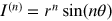 can be seen to contain a saddle point of order n − 1.
Hence when a vortex of order n is disintegrated, there can be many
saddle points appearing as byproducts.
can be seen to contain a saddle point of order n − 1.
Hence when a vortex of order n is disintegrated, there can be many
saddle points appearing as byproducts.
Index is the topological index given to each of the critical points [19]. Since basic topology is beyond the scope of this book, I request readers to assume the topological index values as presented here. For both positive and negative charged vortices of any order, the topological index is +1. Extremum has a topological index +1. An open saddle of order n has topological index of −n and a closed saddle has an index of +n. A saddle that has n + 1 zero crossings has an index of −n and order n.
2.10. Sign rules
Also termed as principles, there are sign principles [20], enlarged sign principles [17] and extended sign principles [21] reported in the literature. The real and imaginary zeros of the wave functions cross each other at the singular point. On real zero contour adjacent singularities are of opposite sign (sign rule). It is also true for imaginary zero contours. But when the real (imaginary) zero contour is going through a saddle point, on either side of it singularities of the same polarity can exist. Application of the (enlarged) sign principle demonstrates that the singularities that terminate on a bifurcation line of an open arm saddle must be of the same sign. Further singularities with the same (opposite) sign terminate bifurcation lines containing an odd (even) number of saddle points.
According to the above rule, the singularities that terminate the bifurcation line of a one-loop saddle are shown to have opposite sign. As the saddle point is traversed twice in passing between the singularities, the bifurcation line contains two saddle points. These sign rules are depicted in figure 2.14.
An important topological constraint involves the signs of adjacent vortices on zero crossings. If two vortices terminate a zero crossing segment containing no saddle points then these two vortices are of opposite sign. But if there is an intervening ordinary first-order saddle, both vortices must have the same sign. This highly useful rule is called the sign principle, which in the form stated is applicable only to generic vortices of any order. It permits one to rapidly determine the relative signs of all vortices on a given set of zero crossings.
The sign principle can be extended to include the case of non-contacting, apparently isolated zero crossings. This can be done by extending either the ZR or ZI line that is crossing a vortex of known charge. If the ZI contour is taken, it is extended till it crosses the (say) ZR that runs through the vortex of unknown charge. Now the sign rule is applied in the extended segment and tracing the charges of the vortices at each of the zero crossings, the polarity of the unknown charge can be determined. This extended sign rule is explained in figure 2.15.

Figure 2.15. Application of the extended sign rule to identify the signs of enclosed vortices C and D. Thick and thin lines are lines of ZR and ZI , respectively. (a) Vortex A is positive and vortex B is negative. (b) and (c) are examples of two different possibilities of contour extensions that permit the sign of the vortex C to be determined as negative and the sign of the vortex D as positive. Reprinted with permission from [21]. Copyright (1994) by the American Physical Society.
Download figure:
Standard image High-resolution image2.11. Disintegrations or explosions
Higher-order critical points are called degenerate critical points. Under the influence of a small perturbation a degenerate critical point can decay explosively into a large number of irreducible non-degenerate components [19]. The mound of debris resulting from decay of a vortex of order 10 as found in superconductors can exceed 5 × 10⁶. These explosions are within the constraints of conservation rules. The index conservation and charge conservations are discussed here.
A higher-order saddle can explode into a large number of first-order saddles and
extrema. An mth order saddle can disintegrate into  first-order saddles and
  extrema. In a phase distribution enriched with phase saddles and
extrema, the phase gradient lines reach and disappear at the saddle in certain
directions and leave from the saddle from other directions. At extrema the phase
gradient lines normally terminate or originate. The phase gradients associated with
phase vortices are circulating in nature around the singular point.
extrema. In a phase distribution enriched with phase saddles and
extrema, the phase gradient lines reach and disappear at the saddle in certain
directions and leave from the saddle from other directions. At extrema the phase
gradient lines normally terminate or originate. The phase gradients associated with
phase vortices are circulating in nature around the singular point.
2.12. Charge conservation
The topological charge of the vortex is a conserved quantity. According to the law of charge conservation, the net charge within some bounded region is conserved under continuous deformation of the wave function, provided that no charges enter or leave the region by crossing the boundary. Therefore, a vortex of charge +5, after disintegration results in the final product of five vortices each with charge +1.
While the charge conservation decides the charge of each of the resulting vortices,
actually the disintegration gives rise to other types of critical points appearing in
the field distribution. An nth order vortex disintegrates into
n2 first-order vortices along with many saddle points and extrema. Out of
these n2 vortices, there are  vortices having one sign and
  vortices having the opposite sign so that the net charge before and
after explosion is conserved [19]. This means that a vortex of charge +6 disintegrates into 21 vortices each
having charge +1 and 15 vortices of charge −1 so that the net charge before and after
explosion is equal to +6.
vortices having the opposite sign so that the net charge before and
after explosion is conserved [19]. This means that a vortex of charge +6 disintegrates into 21 vortices each
having charge +1 and 15 vortices of charge −1 so that the net charge before and after
explosion is equal to +6.
2.13. Index conservation
Index conservation is more important than charge conservation. The net index of critical point(s) before and after disintegration is a conserved quantity. Consider the disintegration of an nth order vortex, that leads to the creation of n2 first-order vortices. Since the topological index of each of the vortices irrespective of the order or sign is +1, the initial index is +1 and the byproduct n2 vortices put together has index n2, hence there should be (n2 − 1) saddles each with topological index (−1) according to the index theorem. Hence +1 = n2 − (n2 − 1) and the index is conserved [19]. If the explosion creates extrema also, it is possible to have more saddles than this number to conserve the topological index.
2.14. Limitation on vortex density
The phase gradient of the vortex is such that at regions near to the core of the vortex very high phase gradients are possible. But having phase vortex dipoles can limit the magnitude of the rapid spatial fluctuation of phase. Accordingly, to avoid rapid spatial fluctuations in phase there exists a kind of limitation on the number of vortices in a given area. Roux [22] has shown that the net topological charge in an area cannot exceed the circumference of that area divided by the wavelength.
In speckle fields which are random vortex fields [20], the vortices are anti-correlated with their nearest neighbors and tend to be uncorrelated with vortices further apart.
The local spatial frequency which is a function of local phase gradient gives an
indication of the angular spectrum of the optical field. The maximum spatial frequency
of a propagating monochromatic wave (wavelength λ) is  . If the average spatial frequency on the contour is larger than
  , at certain regions it indicates that there is a need to have
evanescent waves excited in these regions that do not propagate. Such high vortex
density regions are possible in engineered fields. According to Roux, if
n is the net enclosed topological charge of vortices in a region
surrounded by a boundary of length L, the vortex density limitation
that is applicable is given by
, at certain regions it indicates that there is a need to have
evanescent waves excited in these regions that do not propagate. Such high vortex
density regions are possible in engineered fields. According to Roux, if
n is the net enclosed topological charge of vortices in a region
surrounded by a boundary of length L, the vortex density limitation
that is applicable is given by  .
.
2.15. Threads of darkness
When two beams interfere in space, the interference pattern forms bright and dark surfaces in the volume of overlap. The intersection of these surfaces on a two-dimensional observation plane appears as an interference fringe. Instead of two beams if three or more plane waves whose propagation vectors are non-coplanar interfere, interference makes the light vanish at lines rather than on surfaces. And these dark lines when observed on a two-dimensional plane, appear as dark points instead of fringes and each of these dark points are seen as vortices, where the phase is indeterminate.
These vortices extend in three dimensions as a curve, and are called the threads of darkness. In the context of sound waves, these are called curves of absolute silence. Therefore singular optics can be considered as the study of the dark side of the light.
2.16. Berry's paradox
Reduction of three-dimensional fields to a set of parallel two-dimensional slices is called foliation of the field [23]. These two-diminsional observation planes are called the leaves of the foliation. Normally these leaves of foliation are made in such a way that the foliation and the normal beam axis is 90°, but when this angle is not 90° the observer sees in his leaves different results. Critical foliations are in a way rules and not exceptions as the event is same as that being observed, but viewed from different angles. Isaac Freund terms this paradoxical situation [24] in which nominally equivalent, equally valid experiments produce entirely different results as a 'Berry's paradox'.
Consider the vortex trajectory as shown in figure 2.16 in which the three observation planes are indicated by A, B and C. Depending on which observation plane the observer is using, he will see the presence of a dipole, or singularity-free field. Also as he moves the observation plane from A to B he sees that there is an attractive force between the two vortices that attract each other and at one stage they collide with each other and annihilate. But the foliation shows that there is a single vortex that has formed a loop trajectory whereas the different observers have witnessed different events. Also when the foliations are at different (small) angles, the observations will be completely different. First of all the charge of the vortex as defined in equation (2.5) is no longer required, as the same vortex is considered as a dipole with positive and negative vortices separated by a distance. Hence, what is suggested is that instead of charges we can use directed arrows for the vortices. The arrow directed towards the observer is seen as positive and the arrow directed away from the observer is seen as a negative vortex. Then what about the sign rules? They are still there, and there are two conservation laws, namely vortex topological charge conservation and topological index conservation. These indices are shown conserved under changes in foliation [23].

Figure 2.16. Berry's paradox. The oriented curve is the vortex trajectory. An observer sees that there is an attractive force between the oppositely charged vortices and there is an attraction between them that draws them closer to each other by observing planes A, B and C sequentially.
Download figure:
Standard image High-resolution imageThe location of the vortices in a plane and their trajectories in three dimensions are invariants (foliation-independent). The stationary points computed using zeros and two-dimensional gradients are dependent on the coordinate system used and hence their locations and trajectories in three dimensions are foliation dependent.
Here we simply use the term trajectories to refer to these oriented lines, since much of what follows applies to the general complex field independent of whether or not it is embedded within a wave. As stressed by Berry, the essence of the paradox is that what one sees depends on how one looks, so that different observers examining the same wavefield from different perspectives will see different arrangements of point vortices and will infer different reactions for these points. Berry notes that the problems embedded in the paradox arise whenever a three-dimensional field is described in terms of two-dimensional section foliations. Referring to figure 2.17(a), even though the trajectory of the vortex core is a single one, it is interpreted as a positive vortex in one perspective view and negative vortex from another perspective view and even the single vortex is interpreted as a dipole. Vortex creation and annihilation cannot happen anywhere on the curve. For a single vortex moving along a curved trajectory, how can the vortex charge, which is a topological invariant, change along the trajectory? Hence what is suggested by Freund is that the vortex charge can be dispensed with, by using oriented trajectories.
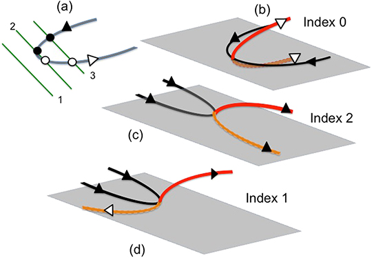
Figure 2.17. Birth and death of vortex pairs along with other critical points. Black and white arrowheads represent vortices of positive and negative charge respectively. Black thick trajectories are for vortices and colored trajectories are for other stationary points (saddles and extrema). The trajectory above the plane of the paper (where vortex trajectory lies) is depicted in red and the trajectory below is depicted in orange. Trajectories in (a) are for charges, (b) for indices, (c) for indices, (d) for indices. In (a) an observer moving along the plane 1, 2, 3 sees the creation of vortex pairs (dipole) hence the net charge is always zero. In (a) the index is not conserved in the three leaves of the foliation. To conserve the index, stationary point trajectories can be added to it, and three different possibilities with different topological indices are discussed in figures (b)–(d). In (b), the observer sees the creation of a vortex dipole along with two saddles as he goes from plane 1 through 3, in this case the index as well as the charge are always zero. In (c), the observer sees a maximum and a minimum transforming into a vortex dipole. Here the charge is zero and the index is always two. In (d) a minimum is transforming into a saddle and a vortex dipole. Here in all the leaves of foliation the net charge is zero and the index is one.
Download figure:
Standard image High-resolution image2.17. Manifolds and trajectories
Vortex trajectories are the curves obtained [25] by the intersection of surfaces of real zero and imaginary zero. These surfaces generally consist of many disconnected pieces. In figure 2.6 some of the real zero and imaginary zero curves obtained by the intersection of these surfaces with the observation plane are shown disconnected. Any of these pieces (surface) is referred as a manifold and can be denoted by R0 or I0. On the surface of the manifold (take any one surface of real zero), continuity, differentiability, and single valuedness of the wave function forbids the presence of holes, slits or any sort of discontinuities. Some of the compact manifolds are shown in figure 2.18. Mathematically, a compact manifold is a manifold which is compact. This definition is not helping us in any way. Maybe, compact means finite and the manifold is a surface. A closed manifold is a compact manifold (surface) without a boundary. Some of the closed compact manifolds are disc, sphere, torus and generalized tori [24]. By defining a genus that indicates the number of holes a surface has, a sphere is a genus zero surface, a donut or torus has genus one. A torus is a sphere with one handle. A sphere with two handles has genus two; it is a coffee cup with two handles. The term 'generalized tori' used by Freund [24] is a surface with genus greater than one. Discs and spheres do not have a handle, whereas a torus has a handle and generalized tori have many handles and none of them have a boundary. An open manifold is a manifold without boundary and hence not compact. All the open edges of the manifolds are at infinity. The vortex trajectory can be seen as a curved line drawn on the surface of R0 without any reference to imaginary zero surface. We can also use I0 surface as a manifold and vortex trajectories on them without reference to real zero surface. These manifolds generally consist of many disconnected pieces. In figure 2.19 a sphere and a cylinder are two manifolds which are disconnected. But one is compact and the other is not. In the observation plane (phase distribution) these two manifolds, are observed as two different circles. In this example they are shown as two different manifolds. Otherwise, (another possibility) through these two circles, a torus can pass through, and these two circles may correspond to one single closed compact manifold.

Figure 2.18. Different types of compact manifolds. First row—simple and compact manifold and equivalent surfaces, second row—torus and equivalent surfaces, and the third row—genus with two surfaces with multiple handles and equivalent surfaces.
Download figure:
Standard image High-resolution image
Figure 2.19. Manifold construction from phase contours drawn on a two-dimensional observation plane. Let us consider a circle which represents a real zero contour line curve in the two-dimensional phase distribution. The real zero contour surface is a cylindrical tube extending to infinity on both directions. This tubular surface is the manifold. Another manifold which is a compact manifold, for the other real zero contour which is disconnected from the other manifold is shown as a sphere. The intersection of the imaginary zero surface with the manifold (cylinder) gives the vortex trajectory.
Download figure:
Standard image High-resolution imageWe have seen earlier that by adding a constant phase to the wave function, one can move the phase contour lines as well as real and imaginary zero lines in a plane. This exercise was done to make any of the phase contours become either a real zero or an imaginary zero curve that can go through the saddle. But at the vortex point this perturbation does not disturb the crossing of real and imaginary zeros. Hence adding a constant phase results in the change of shape of the surfaces R0 and I0, but the same trajectory looks different on the manifold as the shape has now changed. But as far as the trajectory of the vortex core is concerned, it remains the same in three dimensions. We note that the geometry of a vortex trajectory is unchanged by such a transformation, which is referred to as generalized gauge transformation [23, 26]. The orientation of the trajectory also remains invariant under gauge transformation.
Manifolds may be closed (compact) or open that have boundaries at infinity. Spheres, and other closed shapes are compact. A torus and the surface of a tea cup are also compact and each of them can be considered as a sphere with a handle. A generalized tori is a sphere with an arbitrary number of handles. The handles are like bridges that allow the trajectories to cross over each other—like one segment of the trajectory is over the bridge and the other below the bridge. Hence the crossing in a torus helps to create knots. Handles open a route to exotic trajectories which otherwise would be impossible. The trajectory must be on the surface and no part of it is allowed to leave the surface of its manifold.
One open manifold example is a plane with its boundary at infinity. Tube shaped manifolds are also possible in which case the open ends of the tube are located at infinity. Planes and tubes appear to be the generic manifolds in Gaussian laser beams.
Self-intersecting surfaces such as interpenetrating spheres are non-generic and they are excluded from discussion for the sake of simplicity. Under small perturbations, they decompose into two or more independent pieces.
Trajectories
On a plane or on an infinitely long cylinder, both closed and open trajectories are
possible. Trajectories may be simple closed loops, lines that start at say  and end at
  or lines bent into a U with both ends of the U ending at
  . These three types of trajectories are possible on an open
manifold.
. These three types of trajectories are possible on an open
manifold.
On compact manifolds only closed trajectories are allowed. On a torus, which is a compact manifold, three types of closed trajectories namely p, r and t are possible [24]. All these three p-, r- and t-type trajectories are depicted in figure 2.20. The p-type is a closed trajectory that can be shrunk to a point and hence is allowed on all types of manifold. That is the only possible trajectory on a sphere as in a compact manifold only closed trajectories are allowed. The trajectory labelled r is like a ring on a finger and sits on the handle of the torus. The third trajectory labelled t is a closed loop running along and on the surface of torus, mirroring the shape of the torus. If a torus contains only a single trajectory, this must be a p-trajectory. All these three types of closed trajectories on a torus can be resized, slid along the surface of the manifold, rearranged, provided that during this operation the trajectory does not break or open up, leave the surface of the manifold, or cross another trajectory. These operations facilitate the application of the sign rule.

Figure 2.20. (a) Two p-trajectories on the left and one r-trajectory on the right are shown on the surface of a torus. (b) One t-trajectory is shown. (c) Two r-trajectories are shown on the surface of a torus.
Download figure:
Standard image High-resolution imageHaving introduced the types of trajectories, now let us concentrate on the relative orientations of the trajectories. If the orientation (arrowhead) of any one trajectory on a given manifold is known, the orientations of all other trajectories on the manifold can be automatically determined. To find the orientations, the trajectories need to be brought into close proximity with each other.
The sign rule [21, 20] will be satisfied if the arrowheads on two immediately adjacent trajectories point in opposite directions.
p-trajectories The implication of the sign rule is that on any manifold, sets of independent p-trajectories undivided by any other trajectory type, all must have the same orientation, while nested p-trajectories (one inside the other) must have opposite orientations.
r-trajectories For the examination of r-trajectories on a torus or r-trajectories on different handles on a tori, bringing the trajectories in close proximity to each other is difficult as these trajectories cannot be resized or rearranged as done before for p-type trajectories. Hence to bring them closer to each other, we need to make burrows and eventually make a wormhole and connect the trajectories. This process of making a burrow and wormhole is explained in figure 2.21 These burrows are created by pushing and extending the trajectory on the supporting manifold without violating any rule mentioned before and hence are permissible (figure 2.22). This exercise creates two counter-propagating, self cancelling trajectory segments. Then the process of merging the adjacent counter-propagating segment is carried out to form a wormhole. Opening or forming a wormhole merges two trajectories into one while closing the wormhole cuts a single trajectory into two. The arrowheads in all these new trajectories must be consistent and any inconsistency means that the sign rule has been violated. Violation of sign rule happens for two r-trajectories (figure 2.23) with same orientation and two t-trajectories (figure 2.24) with same orientation on a torus and hence these are not allowed. In figure 2.25 violation of sign rule for two r-trajectories with same orientation is explained by using t-trajectories and forming burrows and wormholes.

Figure 2.21. Process of forming a burrow and wormhole.
Download figure:
Standard image High-resolution image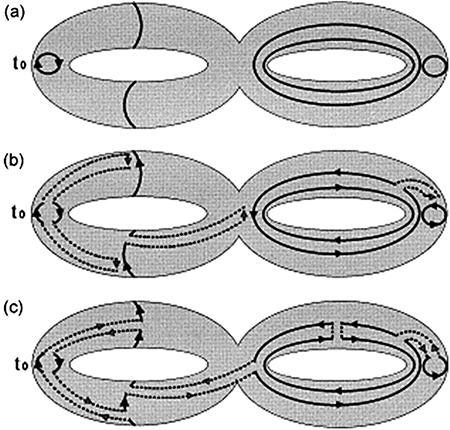
Figure 2.22. Process of forming a burrow and wormhole on a genus two torus that hosts p-, r- and t-type trajectories. Although this process decides the direction of legal arrowheads on every closed trajectories, use of wormholes lead to a single closed trajectory at the end. Reprinted from [24]. Copyright (2000), with permission from Elsevier.
Download figure:
Standard image High-resolution image
Figure 2.23. Two r-trajectories with (a) same orientation is not allowed but (b) forming a null pair is allowed. This has been explained with the help of p-trajectory and by making burrows and wormholes.
Download figure:
Standard image High-resolution image
Figure 2.24. Two t-trajectories with (a) same orientation is not allowed but (b) forming a null pair is allowed.
Download figure:
Standard image High-resolution image
Figure 2.25. Two r-trajectories with same orientation is not allowed. This is shown by using a t-trajectory oriented in two different possible directions (a) and (b). This same example can be used to show that single t-trajectory is not allowed on a torus. By connecting different parts of the t-trajectory using burrows and wormholes formed using pair of r-trajectories, this can be seen.
Download figure:
Standard image High-resolution imaget-trajectory: It is a closed loop running along and on the surface of torus, mirroring the shape of the torus. Sign rule does not allow a single t-trajectory. This has been depicted in figure 2.25. It should appear in pairs on the surface of the torus. In the pair the two trajectories must have opposite orientation and form a null pair as depicted in figure 2.24.
Connecting different parts of the r-trajectory by a t-trajectory wormhole, leads to a contradiction of the direction of the arrowhead. Similarly connecting different parts of the t-trajectory by r-trajectory wormhole, leads to contradiction on arrowhead direction as shown in figure 2.23. Hence a single r- or a single t-trajectory on a handle violates the sign rule (figures 2.25 and 2.26) and is therefore forbidden [24].

Figure 2.26. Single r-trajectory on a torus is not allowed. Using burrows and wormholes made of t-trajectories, it has been explained.
Download figure:
Standard image High-resolution imageTwo counter-propagating trajectories close to one another called null pairs can be inserted anywhere (as long as they do not overlap with other trajectories) on the manifold as they cancel each other and this is tantamount to having no trajectory at all. Higher-order vortices involve self-intersecting manifolds and that analysis is beyond the scope of the book.
In figure 2.22, a genus two torus with two handles is shown. In figure 2.22(a) one p-trajectory is shown on the surface of the left side torus. There are also two r-type trajectories on the same torus. In the second torus which is connected to the first, one p-trajectory and two t-trajectories are shown. From the given orientation of the t0 trajectory one can find the orientations of all other trajectories on the manifold using the process of forming burrows and wormholes as shown in figures 2.22(b) and (c). The orientation of the arrowheads of the trajectories from the knowledge of the initial closed trajectory are unique. This means that there is only one set of correct orientations for the trajectories possible.
2.18. Links and knots
Consider now exotic trajectories on the surface of the manifold. They are spirals, links, and knots. Links and knots are just oriented closed curves.
On compact manifolds trajectories are closed curves (loops) and cannot have a beginning or an end. Such closed trajectories form wavefield dislocation loops. The exotic trajectories such as spirals, links and knots are possible on manifolds with suitable handles.
On a torus t-trajectories must always appear as null pairs. Since an unpaired t-trajectory is not allowed on a torus, linked manifolds cannot give rise to unpaired linked trajectories (figure 2.27). But a null pair on a single torus can form a link. Although the trajectories in the link appear to be t-trajectories, they are in fact counter-propagating r-trajectories. Torus links require only one manifold (either R0 or I0) to be compact.

Figure 2.27. Link formation. (a) Two co-propagating t-trajectories on a torus is not allowed. This can be seen by inserting an observation plane (marked by the dashed line) one can observe that there is a sign rule violation. (b) Hence two counter-propagating t-trajectories called a null pair is allowed on a torus. (c) Link formation by linked manifold with single t-trajectory in each of the torus is not allowed because a torus supports only null pairs. (d) Link formation on a torus. In (d) the two trajectories appear to be t-trajectories and are indeed two counter-propagating r-trajectories.
Download figure:
Standard image High-resolution imageUsing the sign rule, it is easily seen that a spiral trajectory scribed into a torus handle or other closed manifold is forbidden. A single trajectory is scribed into a manifold that is itself twisted into a spiral. The reason for this exclusion is the same as for the exclusion of single r- and t-trajectories on a torus. Spirals constructed from counter-propagating null pairs, however, are always allowed. Since a spiral may be formed by a line scribed into a twisted sheet open manifold, single spirals can be implanted into Gaussian laser beams.
A minimum of three crossings are required to form a knot. Freund [24] has shown that knotted trajectories are not possible on closed manifolds. Violation of the sign rule prevents knot formation in many cases as shown in figure 2.28. Knots of any order formed from counter-propagating null pairs, however, are, as always, allowed. A single t-trajectory is permitted on a non-compact torus, i.e. a torus whose outer circumference has been slit open and the cut edge extended to infinity. A knotted trajectory on a generalized, non-compact higher-order torus therefore remains a possibility.

Figure 2.28. (a) Trefoil knot. (b) Figure of eight knots are not possible as the insertion of the observation plane (shown as dashed line) reveals that the sign rule is violated. (c) Torus knot T23—a higher-order knot is also not allowed. Reprinted from [24]. Copyright (2000), with permission from Elsevier.
Download figure:
Standard image High-resolution imageA random field formed by the interference of scattered coherent light, is shown to have complicated vortex trajectories as shown in figure 2.29. In fact a speckle field is formed due to the interference of light from many scattering points and is a kind of multiple beam interference. Therefore it suggests that complicated vortex trajectories are possible in multiple beam interference. It has been shown by multiple beam interference (figures 2.30 and 2.31) that many of the complicated trajectories are possible [27]. Using coaxial superposition of four or more beams the formation of loops, links and knot structures can be achieved [27–31].

Figure 2.29. Complicated structure of the vortex trajectories in random phase distributions. Reprinted with permission from [32]. Copyright (2009) by the American Physical Society.
Download figure:
Standard image High-resolution image
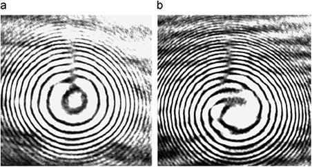
Figure 2.30. Constructing an isolated trefoil knot out of vortex lines in an optical field [29]. (a) In cylindrical geometry it is straightforward to devise a complex-valued function that prescribes where vortex lines, drawn here as two strands, should reside as a function of cylinder height as the strands wind around each other. (b) The braid becomes a knotted loop when the cylinder is topologically mapped into a torus, folding the black loops at the top and bottom onto each other. (c) One can experimentally embed the 'knot' function in an optical field by sending a laser beam through a diffractive hologram that shapes the beam's destructive interference pattern. One can then map out the knot in space by measuring where the phases (shown as different colors in this cross section) become singularities (red). Reprinted by permission from [29]. Copyright (2010) by Springer Nature.
Download figure:
Standard image High-resolution image
Figure 2.31. Experiment to realize knots and links. Knotted lines of darkness. (a) Reconstructed light from the hologram is spatial filtered and a moving camera captures different leaves of foliation. Black lines are threads of darkness that form the link or knot. Inset: over-saturated beam cross-sections at the beam waist of the link with the dark points indicating positions where the optical vortex threads cross the observation plane. (b, c) Three-dimensional representations of measured link (b) and trefoil knot (c) configurations. The link and knot are threaded by further vortices (represented by the thinner tubes) that follow the axis of the light beam. Reprinted by permission from [27]. Copyright (2004) by Springer Nature.
Download figure:
Standard image High-resolution image2.19. Different types of phase defects
Point, edge and mixed phase defects
An optical vortex is a point phase defect. It is also called a wavefront screw dislocation. The wavefront structure looks like a cork-screw and many of its topological aspects were discussed in this chapter. There are also other types like line and mixed type phase defects in a wavefront [4]. In an edge dislocation the phase ambiguity occurs along a line in contrast to the vortex in which the phase ambiguity occurs at an isolated point. This edge dislocated wavefront can be realized by cutting a part of a wavefront and phase shifting it by π. The resulting optical field can be represented by two sets of wavefronts, one shifted from the other by π. The wavefront looks like a step in a staircase. The phase discontinuity here is along a line. The wavefront can be considered to have edge dislocation even when there is phase discontinuity other than π (but not integral multiples of 2π) along the line. In a mixed type dislocation, the indeterminate phase occurs along a line but this ambiguity terminates at a point somewhere in the middle of the wavefront. The point at which the defect terminates is like a point dislocation and the line that terminates on the point is like an edge dislocation. Since both types of defects are present, it is called a mixed type dislocation. It can be considered as a vortex with fractional charge. These three types of phase defect [6] are depicted in figure 2.32. A Burgers vector of wave dislocation can be assigned to these phase defects [33] in analogy with the defects in crystals.

Figure 2.32. (a) Edge, (b) point and (c) mixed type dislocations.
Download figure:
Standard image High-resolution imageIsotropic and anisotropic vortex
An isotropic vortex is the one in which the azimuthal phase gradient is constant. The
phase contour lines that are radial in a vortex are equally spaced azimuthally. In an
anisotropic vortex the azimuthal phase gradient is not constant. As a consequence,
crowding of phase contour lines at some azimuthal angular positions may happen. For
the r-vortex given in equation (2.4) for example, the phase gradient  . Consider the anisotropic vortex [34] given by

The phase variation is given by  and the azimuthal part of the phase gradient is given
by
and the azimuthal part of the phase gradient is given
by

The azimuthal phase gradient can be seen varying in an anisotropic vortex. One can also have other types of non-uniform phase gradients for anisotropic vortices.
Canonical and non-canonical vortex
A canonical vortex is an isotropic vortex and a non-canonical vortex is an anisotropic vortex.
Perfect vortex
In a vortex, the diameter of the dark core increases in size with the charge of the vortex. Higher charge vortices have bigger cores. Perfect vortices are engineered in such a way that the diameter of the vortex core remains the same and is independent of the magnitude of the charge of the vortex. Fourier transformation of Bessel–Gauss (BG) beams of different order is used to generate perfect vortices [35]. These BG beams with vortices in them can be achieved using curved fork gratings [36]. Having a fixed size core allows the beam to maintain good intensity distribution in the donut, and makes it suitable for use in non-linear media [37, 38] as the intensity is linked to the refractive index modulation in such crystals. The fractional charge measurement is possible using phase shifting method [39]. There are also other methods available for perfect vortex generation [40–45].
Fractional vortex
In a vortex the accumulated phase change along a closed path around the vortex is l2π where l is the topological charge. As a consequence there is no phase discontinuity anywhere in the wavefront except at the location of the singularity. If the accumulated phase change along a closed path is not equal to an integral multiple of 2π and is fractional, then the vortex is called a fractional vortex. Hence in a fractional vortex there is a phase discontinuity along a line and this line terminates at a point of undefined phase [46–51]. It is a combination of line and point dislocation and is also termed a mixed type phase dislocation. In a pure edge dislocation there is phase discontinuity along the dislocation line, which means that the wavefront is cut along a line and displaced by a distance less than λ. Hence all along the cut line the phase is singular and this leads to the development of amplitude zero line during propagation. In a mixed type screw dislocation the dark line terminates on the vortex point and hence the donut intensity structure of a integer charged vortex is not there. For a fractional vortex there is a radial intensity cut in the donut structure as shown in figure 2.33.

Figure 2.33. Fractional vortex—simulated diffraction intensity pattern. A radial intensity cut in the donut structure for a fractional vortex of charge (a) 0.5 and (b) 3.5. Reprinted from [49]. Copyright (2010), with permission from Elsevier.
Download figure:
Standard image High-resolution imageWhen multiple fractional charge vortices are present, the dark radial cut pairs with adjacent vortices. This pairing happens irrespective of the polarity of fractional vortex charges. A positive vortex can be connected to another positive vortex or to another negative vortex in the diffraction pattern by dark intensity line as shown in figure 2.34.

Figure 2.34. Top row: Fresnel lens with fractional vortices of the same charge (3.5) embedded at off-axis locations. Bottom row: Fresnel lens with fractional vortices of opposite charge (3.5) embedded at off-axis locations [56]. (a) Phase distribution displayed on SLM. (b) Simulated intensity distribution near the focal plane. (c) Experimentally observed intensity distribution near the focal plane. (d) Distribution of topological charge in the intensity pattern. Reproduced from [56].
Download figure:
Standard image High-resolution imageFractional vortices are unstable structures. During propagation along the dark line that is breaking the circular symmetry of the donut structure, a series of integer charged vortices are produced. They are in the form of dipole chains, and these multiple vortices are arranged along the dark line. The intensity distribution in the focal plane of fractional vortex lenses are examined by interference with a plane wave and fringe pattern with multiple forks pointing in opposite directions can be observed as shown in figure 2.35. This confirms the presence of multiple vortices with alternating signs in the radial cut.
Figure 2.35. Fractional vortex–diffraction. Reprinted from [49]. Copyright (2010), with permission from Elsevier.
Download figure:
Standard image High-resolution image
Riemann–Silberstein vortex
Over a century ago Ludwick Silberstein [52] introduced a new vector, which was later known as the Riemann–Silberstein (RS) vector given by

where  are electric and magnetic field vectors and c is
the velocity of light. This RS vector simplifies many problems in EM theory and is a
very useful tool. The circularly polarized plane wave can be written as
are electric and magnetic field vectors and c is
the velocity of light. This RS vector simplifies many problems in EM theory and is a
very useful tool. The circularly polarized plane wave can be written as

The total energy is written as the norm of 

The use of the RS vector greatly simplifies the description of the electromagnetic fields [53]. Vortices present in such RS vector fields are called Riemann–Silberstein vortices [54, 55].
References
- [1]Nye J F and Berry M V 1974 Dislocation in wave trains Proc. R. Soc. Lond. Ser. A 336 165–90
- [2]Baranova N B, Mamaev A V, Pilipetsky N F, Shkunov V V and Ya Zel'dovich B 1983 Wavefront dislocations: topological limitations for adaptive systems with phase conjugation J. Opt. Soc. Am. 73 525–9
- [3]Bazhenov V Y, Vasnetsov M V and Soskin M S 1990 Laser beams with screw dislocation in their wavefronts JETP Lett. 52 429–31
- [4]Basisty I V, Soskin M S and Vasnetsov M V 1993 Optics of light beams with screw dislocations Opt. Commun. 103 422–8
- [5]Freund I, Shvartsman N and Freilkher V 1993 Optical dislocation network in highly random media Opt. Commun. 101 247–64
- [6]Basistiy I V, Soskin M S and Vasnetsov M V 1995 Optical wavefront dislocations and their properties Opt. Commun. 119 604–12
- [7]Soskin M S, Gorhkhov V N, Vasnetsov M V, Malos J T and Heckenberg N R 1997 Topological charge and angualr momentum of light beams carrying optical vortices Phys. Rev. A 56 4064–75
- [8]Bazhenove V Y U, Soskin M S and Vasnetsov M V 1992 Screw dislocations in light wavefronts J. Mod. Opt. 39 985–90
- [9]Soskin M S and Vasnetsov M V 2001 Singular optics Progress in Optics vol 42
- [10]Ghai D P, Senthilkumaran P and Sirohi R S 2008 Shearograms of optical phase singularity Opt.Commun. 281 1315–22
- [11]Kowaz M W 1995 Homogeneous and evanescent contributions in scalar near-field diffraction Appl. Opt. 34 3055–63
- [12]Berry M V 1994 Faster than Fourier in Quantum coherence and Reality (Singapore: World Scientific) 55–65
- [13]Lochab P, Senthilkumaran P and Khare K 2016 Near-core structure of a propagating optical vortex J. Opt. Soc. Am. A 33 2485–90
- [14]Berry M V 2008 Conf. on Coherence and Quantum Optics (Washington DC: OSA) 37–41
- [15]Berry M V 2005 Phase vortex spirals J. Phys. Math. Gen. 38 L745–51
- [16]Senthilkumaran P and Bahl M 2015 Young's experiment with waves near zeros Opt. Express 23 10968–73
- [17]Freund I 1995 Saddles, singularities, and extrema in random phase fields Phys. Rev. E 52 2348–60
- [18]Freund I 1999 Saddle point wave fields Opt. Commun. 163 230–42
- [19]Freund I 1999 Critical point explosions in two-dimensional wave fields Opt. Commun. 159 99–117
- [20]Shvartsman N and Freund I 1994 Vortices in random wave fields: Nearest neighbor anticorrelations Phys. Rev. Lett. 72 1008–11
- [21]Freund I and Shvartsman N 1994 Wave-field phase singularities: the sign principle Phys. Rev. A 50 5164–72
- [22]Roux F S 2003 Optical vortex density limitation Opt. Commun. 223 31–7
- [23]Freund I 2001 Critical foliations Opt. Lett. 26 545–7
- [24]Freund I 2000 Optical vortex trajectories Opt. Commun. 181 19–33
- [25]Berry M V and Dennis M R 2000 Phase singularities in isotropic random waves Proc. R. Soc. Lond. Ser. A 456 2059–79
- [26]Freund I 2001 Critical foliations and Berry's paradox Opt. Photon. News 12 56
- [27]Leach J, Dennis M R, Courtial J and Padgett M J 2004 Knotted threads of darkness Nature 432 165
- [28]Wilson M 2010 Hologram tie optical vortices in knots Phys. Today 63 18–20
- [29]Dennis M R, King R P, Jack B, O'Holleran K and Padgett M J 2010 Isolated optical vortex knots Nat. Phys. 6 118–21
- [30]Leach J, Dennis M R, Courtial J and Padgett M J 2005 Vortex knots in light New J. Phys. 7 1–11
- [31]Dennis M R 2009 Topological configurations of optical phase singualrities Topologica 2 1–10
- [32]Holleran K O, Dennis M R and Padgett M J 2009 Topology of light's darkness Phys. Rev. Lett. 102 143902
- [33]Dennis M R 2009 On the burgers vector of a wave dislocation J. Opt. A: Pure Appl. Opt. 11 094002
- [34]Kim G-H, Lee H J, Kim J-U and Suk H 2003 Propagation dynamics of optical vortices with anisotropic phase profiles J. Opt. Soc. Am. B 20 351–9
- [35]Ostrovsky A S, Rickenstorff-Parrao C and Arrrizon V 2013 Generation of the perfect optical vortex using a liquid-crystal spatial light modulator Opt. Lett. 38 534–6
- [36]Karahroudi M K, Parmoon B, Qasemi M, Mobashery A and Saghafifar H 2017 Generation of perfect optical vortices using a Bessel–Gaussian beam diffracted by curved fork grating Appl. Opt. 56 5817–23
- [37]Chaitanya N A, Jabir M V and Sharma G K 2016 Efficient nonlinear generation of high power, high order, ultrafast perfect vortices in green Opt. Lett. 41 1348–51
- [38]Jabir M V, Chaitanya N A, Aadhi A and Sharma G K 2016 Generation of perfect vortex of variable size and its effects in angular spectrum of the down-converted photons Sci. Rep. 6 1–8
- [39]Ma H, Li X, Tai Y, Li H, Wang J, Tang M, Wang Y, Tang J and Nie Z 2017 In situ measurement of the topological charge of a perfect vortex using the phase shift method Opt. Lett. 42 135–8
- [40]Garca-Garca J, Rickenstorff-Parrao C, Ramos-Garcia R, Arrizon V and Ostrovsky A S 2014 Simple technique for generating the perfect optical vortex Opt. Lett. 39 5305–8
- [41]Oemrawsingh S S R, Eliel E R, Woerdman J P, Verstegen E J K, Kloosterboer J G and 't Hooft G W 2004 Half-integral spiral phase plates for optical wavelengths J. Opt. A: Pure Appl. Opt. 6 S288
- [42]Kotlyar V V, Kovalev A A and Porfirev A P 2016 Optimal phase element for generating a perfect optical vortex J. Opt. Soc. Am. A 33 2376–84
- [43]Chen Y, Fang Z-X, Ren Y-X, Gong L and Lu R-D 2015 Generation and characterization of a perfect vortex beam with a large topological charge through a digital micromirror device Appl. Opt. 54 8030–5
- [44]Deng D, Li Y, Han Y, Su X, Ye J, Gao J, Sun Q and Qu S 2016 Perfect vortex in three-dimensional multifocal array Opt. Express 24 28270–8
- [45]Fu S, Wang T and Gao C 2016 Perfect optical vortex array with controllable diffraction order and topological charge J. Opt. Soc. Am. A 33 1836–42
- [46]Baistiy I V, Pasko V A, Slyusar V V, Soskin M S and Vasnetsov M V 2004 Synthesis and analysis of optical vortices with fractional topological charges J. Opt. A: Pure Appl. Opt. 6 S166–9
- [47]Berry M V 2004 Optical vortices evolving from helicoidal integer and fractional phase steps J. Opt. A: Pure Appl. Opt. 6 259–68
- [48]Lee W M, Yaun X-C and Dholakia K 2004 Experimental observation of optical vortex evolution in a Gaussian beam with an embedded fractional phase step Opt. Commun. 293 129–35
- [49]Vyas S, Singh R K and Senthilkumaran P 2010 Fractional vortex lens Opt. Laser Technol. 42 1150–9
- [50]Singh B K, Mehta D S and Senthilkumaran P 2013 Visualization of internal energy flows in optical fields carrying a pair of fractional vortices J. Mod. Opt. 60 1027–36
- [51]Sharma M K, Joseph J and Senthilkumaran P 2014 Fractional vortex dipole phase filter Appl. Phys. B 117 325–32
- [52]Silberstein L 1907 Grundgleichungen in bivectorieller behandlung Ann. Phys. 22 579
- [53]Bialynicki-Birula I and Bialynicka-Birula Z 2013 The role of the Riemann-Silberstein vector in classical and quantum theories of electromagnetism J. Phys. A: Math. Theor. 46 053001
- [54]Berry M V 2004 Riemann-Silberstein vortices for paraxial waves J. Opt. A. Pure Appl. Opt. 6 S175–7
- [55]Kaiser G 2003 Helicity, polarization and Riemann-Silberstein vortices J. Opt. A. Pure Appl. Opt. 6 S243–5
- [56]Vyas S, Singh R K, Ghai D P and Senthilkumaran P 2012 Fresnel lens with embedded vortices Int. J. Opt. 2012 249695