The basic concepts of classical physics as a useful path towards modern physics
Published August 2020
•
Copyright © IOP Publishing Ltd 2020
Pages 1-1 to 1-35
You need an eReader or compatible software to experience the benefits of the ePub3 file format.
Download complete PDF book, the ePub book or the Kindle book

Permissions
Abstract
In this chapter, we review the fundamental concepts of classical physics with the aim of clarifying some delicate points that need to be fully understood in view of their application to modern physics. In the first part, Newton's principles of dynamics, with a list of pedagogical examples, are illustrated, together with the concepts of work, energy and angular momentum. Connections between symmetries and conservation laws are also discussed. The second part of the chapter is devoted to the Maxwell equations, with a focus on how they lead to the prediction of electromagnetic waves that can travel through space.
Classical physics includes all the theories formulated after the seventeenth and before the twentieth century, characterized by the implementation of the scientific method proposed by Galileo Galilei [1]. From that moment, nature was investigated by scientists under a completely new perspective. The key feature of classical physics is undoubtedly the determinism which characterizes all its fields, from celestial mechanics to electrodynamics. According to Pierre Simon Laplace, 'an intelligence knowing all the forces acting in nature at a given instant, as well as the momentary positions of all things in the Universe, would be able to comprehend in one single formula the motions of the largest bodies as well as the lightest atoms in the world ... nothing would be uncertain, the future as well as the past would be present to its eyes' [2].
The birth of quantum mechanics and the theory of relativity in the twentieth century undermined that vision of the Universe and created the crisis of classical physics, highlighting the need to adopt a totally different point of view (see chapters 3, 7 and 8). However, deep knowledge of the concepts of classical physics cannot be avoided if one is to understand modern physics. In fact, a physicist's mindset is shaped at the beginning when it approaches classic physics. In this chapter, our intent is to present some of the constitutive topics of classical physics, reworked in an educational manner; we propose alternative approaches to the canonical methods, in order to highlight their relevance to students and to prepare them for the study of modern physics. Moreover, the choice of subjects here has been made by considering each of them as preparatory and useful for the comprehension of the subsequent subjects.
In section 1.1 we introduce the three principles of dynamics with the purpose of underlining their conceptual value and their revolutionary importance. Section 1.2 deals with the concepts of work and energy, putting in evidence the strong correlation between these two quantities; in addition, profound knowledge of the classical concept of energy allows its quantization in quantum mechanics to be understood even more. This motivation, namely the 'quantum jump' which characterizes certain physical quantities, is also the reason why section 1.3 is devoted to the introduction of the momentum of a vector. In particular, angular momentum is generally a difficult concept for students; therefore we propose a pedagogical path in order to make it easier to understand. Section 1.4 is dedicated to a fundamental argument, which is hardly ever taken into account in basic physics courses, despite its unquestionable relevance: the link between symmetries and conservation laws, as investigated within the celebrated Noether theorem. Finally, sections 1.5 and 1.6 are devoted to the concept of the wave and to Maxwell's equations, respectively, showing how it is possible to teach students that an undulatory behaviour for coupled electric and magnetic fields can, under suitable conditions, be predicted. We propose an alternative way to present this topic by introducing the concepts of divergence and curl of a vectorial field in a simplified but correct perspective.
It should be noted that in this context we mostly deal with mechanics rather than thermodynamics or electrodynamics. Actually, we believe that stressing these subjects is significant, since by learning to handle classical mechanics it is possible to acquire an universal method which turns out to be useful in every field of physics (and not only in physics) [3].
1.1. The Newton principles of dynamics
1.1.1. The principle of relativity and the first principle
According to Aristotle, the natural state of bodies is rest; thus, any body in movement tends to get slower and slower until it stops, unless it is pushed to continue its motion. Aristotle reached this conclusion, which is evidently wrong, based on his experiments. On the other hand, Galileo interpreted the same experiments in a completely different way: if the object tends to slow down then there is a force opposed to its motion, called the force of friction. He recognized (for the first time) the rank of 'force' for the phenomenon of friction. The difference between the two approaches is undoubtedly the scientific method used by Galileo; through it, the Aristotelian false belief about motion was corrected and the results can be summarized in the following statements:
- 1.If two laboratories move with uniform linear motion, no experiment will give different results in either of them.
- 2.A reference system moving with uniform linear motion is defined as inertial.
- 3.In an inertial reference system, a physical object preserves its rest or its uniform linear motion if it is not forced to change this state by the application of an external force.
The first point is the well-known principle of relativity. Point 3 is the principle of inertia, formulated by referring to the definition of an inertial reference system given in point 2. It should be noted that 'force' is intended here as a 'real force', i.e. an interaction due to something with physical relevance. A fictitious force, in contrast, is the product of the mass of the object through a non-inertial contribution to the acceleration that may emerge in the reference system in which it is located.
The first principle has revolutionary value: it states that the state of rest and the state of uniform linear motion are indistinguishable. This bold assertion is not simple to accept, since it is contrary to common intuition. The first principle also has a fundamental conceptual value, since it allows a special class of reference systems to be defined, that is, the inertial systems.
However, it also has a logical irregularity: according to its formulation, in order to know if one reference system is inertial we have to assure that no forces act on an object in it. Then, we have to verify the state of motion of the object: if it is at rest or moves with a constant speed, the reference system is inertial, otherwise, if it moves with a finite acceleration the reference system is not inertial. However, this demands certainty that no real force is acting on it, but this is formally impossible, since we do not have a quantitative definition of what we mean when we say that a force is zero. We can use the first principle 'back to front', namely as a principle allowing us to deduce whether a net force acts on an object. This, however, requires knowing that one is in an inertial system, so that one definitely ends up with a circular definition. In order to overcome this difficulty, it is assumed that an inertial reference system by definition exists, having its origin in the Sun and its axes oriented toward the fixed stars. As a consequence, all reference systems which are at rest or which move with constant speed with respect to this inertial system are inertial as well. In this way, once an inertial reference system is selected, one can immediately establish if some net forces act on a given object, by checking if it is at rest or in a state of uniform linear motion. It is clear that, under these conditions, the first principle can be used as a criterion to verify the presence or the absence of forces.
1.1.2. The second principle
The second principle deals with the concept of force. It was formulated by Isaac Newton who had in mind real forces only. There are several misconceptions about forces, which can be pointed out by asking students the following questions:
- 1.Do we need contact to exert a force?
- 2.Does the application of a force move an object?
- 3.If an object moves under the action of a force, does it always move in the same direction of the applied force?
Everyday experience leads to incorrect answers to these questions, in particular to the second one: students are tempted to answer 'yes' since they confuse the concept of force with the concept of energy: work always implies motion, whereas the same cannot be said for a force.
The first misconception can be immediately removed if we refer to well-known examples, such as the gravitational force or the electrostatic interaction, which demonstrate that contact is not necessary to exert a force on an object.
The answer to the second question can be suggested by pushing a desk and observing that it does not move if the applied force is not sufficient to overcome the maximum static friction force. Thus, it is evident to students that the application of a force does not always generate motion.
The third point is probably the most subtle, as one can understand on the basis of the following example: there is an attractive force between the Earth and the Moon and it is directed along the line which links their centres, however, the Moon does not move toward the centre of the Earth. Why does this happen? The answer is that the application of a force makes a body acquire an acceleration which is always parallel to the force, but this does not imply that its displacement, i.e. its velocity, is parallel to the force too.
The innovative significance of the second principle is that it establishes the real
relation between the cause of the motion (a force
 doing finite work) and its effect (the
acceleration
doing finite work) and its effect (the
acceleration  ). Since it predicts what happens when
causes are known, it introduces the profound concept of determinism, which is
important also from a philosophical point of view: specifying position and speed at a
given time, the equation
). Since it predicts what happens when
causes are known, it introduces the profound concept of determinism, which is
important also from a philosophical point of view: specifying position and speed at a
given time, the equation
 gives the possibility of describing the
motion of an object completely. This point is crucial and characterizes classical
mechanics, differently to what happens in quantum mechanics. The second principle has
also an important conceptual significance, since it allows the mass of an object to be
defined, beyond Newton's idea that it simply denotes the quantity of matter. The
second principle refines this interpretation and defines the mass as the ratio between
the modulus of the net force applied to an object and the modulus of the acceleration
that it acquires. This ratio identifies the so-called inertial mass of an object,
which is different to the gravitational mass, i.e. the property which we measure with
a weight scale. Nevertheless, it is proved rigorously that for the same object the two
values are the same.
gives the possibility of describing the
motion of an object completely. This point is crucial and characterizes classical
mechanics, differently to what happens in quantum mechanics. The second principle has
also an important conceptual significance, since it allows the mass of an object to be
defined, beyond Newton's idea that it simply denotes the quantity of matter. The
second principle refines this interpretation and defines the mass as the ratio between
the modulus of the net force applied to an object and the modulus of the acceleration
that it acquires. This ratio identifies the so-called inertial mass of an object,
which is different to the gravitational mass, i.e. the property which we measure with
a weight scale. Nevertheless, it is proved rigorously that for the same object the two
values are the same.
In the following, we report three more widespread student beliefs that turn out to be false.
- Students often believe that gravity does not act in a vacuum; therefore, for
example, in their opinion astronauts float in a spaceship because they are in a
vacuum. This is of course not true: this actually happens because the spaceship
is subject to gravity in exactly the same way as the astronauts are, in the
sense that they are both in free fall. In order to clarify this concept, let us
consider a lift and a student in it. For an inertial observer, we have that the
projection of
 along the vertical direction leads
towhere N is the normal force, T is the tension of the cable, a is the acceleration of the lift and is the acceleration of gravity
(G is the gravitational constant,
MT
is the mass of Earth and
r is the distance of the student from the centre of the
Earth). Then, from equation (1.1) it follows that: If the cable of the lift breaks (T = 0), then the lift is in free fall; this means that a = g and, as a consequence, N = 0, i.e. the previous contact between the student's feet and the lift floor ceases to exist (see figure 1.1). The student, then, begins to float, since he is falling and the lift is falling in exactly the same way. This is what happens to the astronauts in the spaceship, namely the astronauts and the spaceship are together in free fall around the Earth.
along the vertical direction leads
towhere N is the normal force, T is the tension of the cable, a is the acceleration of the lift and is the acceleration of gravity
(G is the gravitational constant,
MT
is the mass of Earth and
r is the distance of the student from the centre of the
Earth). Then, from equation (1.1) it follows that: If the cable of the lift breaks (T = 0), then the lift is in free fall; this means that a = g and, as a consequence, N = 0, i.e. the previous contact between the student's feet and the lift floor ceases to exist (see figure 1.1). The student, then, begins to float, since he is falling and the lift is falling in exactly the same way. This is what happens to the astronauts in the spaceship, namely the astronauts and the spaceship are together in free fall around the Earth. - In order to point out a common mistake, sometimes reported in considerations of
the physics of sport, one can consider the case of a ball hit by a racket; in
the study of the motion of the ball, the force that the racket exerts on it must
not be included in the equation
, because this force only affects the
initial conditions of the motion, determining the value of the initial velocity
0. More precisely, we deal
in this case with an impulsive force acting during a very short time interval
, which causes a variation of the
quantity of motion in one dimension, given by
- Consider a pendulum and the projection of
in the direction of the cable; in
some cases students are tempted to write since there is no motion along the cable. Obviously, this is wrong since the normal component of the acceleration is clearly non-vanishing.


![$\mathit{\unicode[Book Antiqua]{x76}}$](https://content.cld.iop.org/books/10__1088_978-0-7503-2678-0/revision2/bk978-0-7503-2678-0ch1ieqn22.gif)


Figure 1.1. (a) A student in a lift going down and (b) the same system in free fall when the cable is broken.
Download figure:
Standard image High-resolution image1.1.2.1. Most common errors
In this subsection, we discuss some common mistakes made by students in the application of the second principle of dynamics. This aspect should be taken into consideration: it is important to show students what should be done and what should not. In our opinion, students should be encouraged in particular when they get something wrong, since errors can be useful in order to obtain complete comprehension. In the left panel of figure 1.2, we show a mistake in writing the second law of dynamics, while the panels in the centre and on the right relate to two widespread errors with regard to the formal definition of the force of friction and the acceleration of an object on an inclined plane, respectively. Another misleading belief of students is that the so-called centrifugal force is an active force pushing an object out of its trajectory. This is obviously false, since it is a fictitious force, i.e. not due to a real interaction, that appears to act on an object when viewed in a rotating frame of reference. Some confusion may also arise with the concept of centripetal force, which students in some cases consider as a specific applied force. In contrast, the real physical quantity to refer to is the centripetal acceleration: when it is non-vanishing, then the product of mass for acceleration is the force, which sometimes is a tension, sometimes a reaction constraint, and so on.

Figure 1.2. Serious mistakes in writing the second law of dynamics (left), the force of friction (centre) and the force of gravity on a inclined plane (right).
Download figure:
Standard image High-resolution imageGenerally speaking, the most frequent errors are related to the use of vectors, which apparently often causes difficulties for students. In figures 1.3 and 1.4, we report other mistakes, in this case concerning the scalar and the vectorial products and the definition of pressure, respectively. In particular, the image on the right in figure 1.4 shows a double mistake: the first is, of course, that pressure is not a vector; the second one deals with the fact that, in vector algebra, the inverse of a vector is not defined (note that this mistake is also present in the image on the left of figure 1.2).

Figure 1.3. Two mistakes for the scalar and the vectorial product.
Download figure:
Standard image High-resolution image
Figure 1.4. Incorrect relations defining pressure.
Download figure:
Standard image High-resolution image1.1.3. The third principle
An important aspect of the third principle is that opposite forces between two particles act along the same straight line. Without this clarification, in several cases students could be misled. For example, by considering an isolated system with two particles, the conservation of the linear momentum gives:

where
 is the force that
m2 exerts on m1 and
is the force that
m2 exerts on m1 and
 is the force that
m1 exerts on m2. One could
thus be tempted to conclude that the third principle is a consequence of the second
one, but this is not true since equation (1.2) does not imply that
is the force that
m1 exerts on m2. One could
thus be tempted to conclude that the third principle is a consequence of the second
one, but this is not true since equation (1.2) does not imply that
 and
and
 act along the same line. A possible
suggestion to give to students is that every time we individuate a force acting on an
object, there is always its partner, as required by the third principle; however, it
is important to remember that the correct partner is not included in the equation of
motion of the object we are interested in. A check on this point could be to ask a
student: 'Consider an object lying on a table. Is the normal force exerted by the
table on the object the partner of the weight on the object?'. Frequently the student
answers 'yes', but this is the wrong answer, because the partner is the force exerted
by the object on the Earth.
act along the same line. A possible
suggestion to give to students is that every time we individuate a force acting on an
object, there is always its partner, as required by the third principle; however, it
is important to remember that the correct partner is not included in the equation of
motion of the object we are interested in. A check on this point could be to ask a
student: 'Consider an object lying on a table. Is the normal force exerted by the
table on the object the partner of the weight on the object?'. Frequently the student
answers 'yes', but this is the wrong answer, because the partner is the force exerted
by the object on the Earth.
1.2. Work and energy
1.2.1. The concept of work
The concept of work is a central one, since it is strictly related to the concepts of kinetic and potential energy. This is of course of special relevance, since every form of energy (thermal, electric or nuclear) is always attributable to the forms of kinetic and potential energies of the elementary constituents. The importance of the concept of work is thus undoubted, thus it should be introduced in basic mechanics courses in a careful and appropriate way. The fundamental definition of work should be referred to the simplest situation, i.e. constant force and linear displacement; under these conditions, it is defined as the product between the force and the displacement which the force generates in the direction of the force itself. This means that all the forces giving rise to displacements orthogonal to their own direction do not produce work. This is what happens, for instance, in the case of a force acting on a particle which moves in a uniform circular motion. In contrast, if the force and the displacement are in the same direction, the work is maximum: this is what happens, for example, when a force pushes an object on a constraint in the direction parallel to the constraint. An elegant way to express this concept is the use of the scalar product:

Here θ
is the angle formed by the direction of the force
 and the direction of the displacement
 . This definition, which, as already stated,
refers to the special case of constant force and linear displacement, can be
immediately used to give the definition of work in the general case of variable forces
and curvilinear trajectories. It is sufficient to divide a given trajectory
C into a series of elements small enough that they can be
considered linear and that the force along each of them can be assumed to be
approximately constant. The general procedure is illustrated in figure 1.5, where the red vectors
represent generic displacements
. This definition, which, as already stated,
refers to the special case of constant force and linear displacement, can be
immediately used to give the definition of work in the general case of variable forces
and curvilinear trajectories. It is sufficient to divide a given trajectory
C into a series of elements small enough that they can be
considered linear and that the force along each of them can be assumed to be
approximately constant. The general procedure is illustrated in figure 1.5, where the red vectors
represent generic displacements
 (
( ) along the elements into which the
trajectory has been divided. Under the conditions specified above, the definition
(1.3) can be
applied to each linear element, so that one can introduce the sum
) along the elements into which the
trajectory has been divided. Under the conditions specified above, the definition
(1.3) can be
applied to each linear element, so that one can introduce the sum

Work is then defined as the limit of this quantity when the number of elements into which the trajectory has been divided becomes arbitrarily large or, equivalently, the length of each them becomes arbitrarily small:

The integral in
equation (1.4)
refers to a calculation along a line; indeed, the subscript C denotes
that the result of the integral is intimately connected to the path along which the
calculation is performed. This is a point to stress with students, since the symbol
 is also used to indicate ordinary
integrals, defined, according to figure 1.6, as
is also used to indicate ordinary
integrals, defined, according to figure 1.6, as

It is evident that whereas the above quantity is only related to the dependence of F on x, in equation (1.4) the result is also dependent on the path C. Thus, equations (1.4) and (1.5) are profoundly different in their significance. Integrals such as the one in equation (1.4) are called line integrals to point out the importance of the path for their evaluation, while integrals such as that in equation (1.5) are the ordinary Riemann integrals. We also point out that when the line integral of a given vector is calculated around a loop, the integral is often called circulation of the vector.

Figure 1.5. Illustration of the calculation of a line integral.
Download figure:
Standard image High-resolution image
Figure 1.6. Illustration of the calculation of a definite integral.
Download figure:
Standard image High-resolution imageIn this context, it is worth mentioning a special case: the work done by a fluid as a consequence of variations of its volume, as usually considered in thermodynamics. The line integral, in this case, becomes an ordinary integral and the work reads

where
 and
and
 are the values of V in the
initial and final equilibrium states A and B, respectively. In the above expression,
are the values of V in the
initial and final equilibrium states A and B, respectively. In the above expression,
 is the pressure of the fluid, with
F⊥ being the force orthogonal to its surface and
A is the section of the recipient which contains the fluid, taken
parallel to its surface. This integral is graphically represented in figure 1.7.
is the pressure of the fluid, with
F⊥ being the force orthogonal to its surface and
A is the section of the recipient which contains the fluid, taken
parallel to its surface. This integral is graphically represented in figure 1.7.

Figure 1.7. Representation of the thermodynamic work in the P–V plane.
Download figure:
Standard image High-resolution imageLine integrals are a widely used mathematical tool. The definitions of the electric potential difference and the Ampère circuital law, for example, are expressed in terms of line integrals:

Going back to equation (1.4), it is evident that the value of a line integral is a function of the chosen path. However, there exists a special category of forces, called conservative forces, for which the line integral is independent of the path and only depends on its initial and final points. In these special cases, one introduces a function V which allows the result of the line integral to be written in the form

whatever the line C connecting the initial and the final points i and f, such that the integral only depends on i and f. In addition, if the initial point i is kept fixed, equation (1.6) allows each point of the space to associate to a number, that is, the work done by the conservative force when a particle moves from i to that point (we deal with this argument in more detail in the next section). This also implies that if we choose a closed line, the value of the integral is always zero.
1.2.2. The concept of kinetic energy
Kinetic energy is defined as the energy of an object of mass m in
movement with speed equal to
![$\mathit{\unicode[Book Antiqua]{x76}}$](https://content.cld.iop.org/books/10__1088_978-0-7503-2678-0/revision2/bk978-0-7503-2678-0ch1ieqn47.gif) and it is expressed as
and it is expressed as
![$K=\frac{1}{2}{m\mathit{\unicode[Book Antiqua]{x76}}}^{2}$](https://content.cld.iop.org/books/10__1088_978-0-7503-2678-0/revision2/bk978-0-7503-2678-0ch1ieqn48.gif) . It can be useful to motivate such a
definition by showing students its origin and the important link with the concept of
work illustrated in the previous section.
. It can be useful to motivate such a
definition by showing students its origin and the important link with the concept of
work illustrated in the previous section.
Let us consider a particle of mass m and all the forces acting on
it. If we define  as the sum of all these forces, the second
principle of dynamics asserts that
as the sum of all these forces, the second
principle of dynamics asserts that
 , where
 is the acceleration of the particle. Then,
we can calculate the work
is the acceleration of the particle. Then,
we can calculate the work
 done by
 relative to a displacement from point A to
point B:
relative to a displacement from point A to
point B:

Here, starting from
![$\vec{\mathit{\unicode[Book Antiqua]{x76}}}=\frac{{\rm{d}}\vec{s}}{{\rm{d}}t}$](https://content.cld.iop.org/books/10__1088_978-0-7503-2678-0/revision2/bk978-0-7503-2678-0ch1ieqn55.gif) , we have used
, we have used
![${\rm{d}}({\mathit{\unicode[Book Antiqua]{x76}}}^{2})={\rm{d}}(\vec{\mathit{\unicode[Book Antiqua]{x76}}}\cdot \vec{\mathit{\unicode[Book Antiqua]{x76}}})=\vec{\mathit{\unicode[Book Antiqua]{x76}}}\cdot {\rm{d}}\vec{\mathit{\unicode[Book Antiqua]{x76}}}+{\rm{d}}\vec{\mathit{\unicode[Book Antiqua]{x76}}}\cdot \vec{\mathit{\unicode[Book Antiqua]{x76}}}$](https://content.cld.iop.org/books/10__1088_978-0-7503-2678-0/revision2/bk978-0-7503-2678-0ch1ieqn56.gif) , so that
, so that
![${\rm{d}}({\mathit{\unicode[Book Antiqua]{x76}}}^{2})=2\vec{\mathit{\unicode[Book Antiqua]{x76}}}\cdot {\rm{d}}\vec{\mathit{\unicode[Book Antiqua]{x76}}}$](https://content.cld.iop.org/books/10__1088_978-0-7503-2678-0/revision2/bk978-0-7503-2678-0ch1ieqn57.gif) . The calculation in equation (1.7), which
expresses the so-called work–energy theorem, shows that the work done by all forces
acting on a particle equals the variation of a quantity,
. The calculation in equation (1.7), which
expresses the so-called work–energy theorem, shows that the work done by all forces
acting on a particle equals the variation of a quantity,
![$K=\frac{1}{2}{m\mathit{\unicode[Book Antiqua]{x76}}}^{2}$](https://content.cld.iop.org/books/10__1088_978-0-7503-2678-0/revision2/bk978-0-7503-2678-0ch1ieqn58.gif) , depending on the modulus of the velocity,
defined as the kinetic energy of the particle. The above result is also valid in
special relativity [4].
Writing the force as
, depending on the modulus of the velocity,
defined as the kinetic energy of the particle. The above result is also valid in
special relativity [4].
Writing the force as

and calculating the derivative explicitly, we obtain

Given this expression
of the relativistic force
 , we can evaluate the elementary work
 . After some simple algebra, we
obtain
. After some simple algebra, we
obtain

This expression can also be written in the form

We can now evaluate the
finite work  done by
 when a particle moves from A to B by
integrating equation (1.8):
when a particle moves from A to B by
integrating equation (1.8):

This result allows the relativistic kinetic energy to be defined as

where
K0 is a constant. By imposing the condition
![$K(\mathit{\unicode[Book Antiqua]{x76}}=0)=0$](https://content.cld.iop.org/books/10__1088_978-0-7503-2678-0/revision2/bk978-0-7503-2678-0ch1ieqn69.gif) one immediately finds
one immediately finds
 , so that the final expression of the
relativistic kinetic energy is
, so that the final expression of the
relativistic kinetic energy is

It is worth noting
that, expanding this expression in Taylor series for
![$\mathit{\unicode[Book Antiqua]{x76}}/c\ll 1$](https://content.cld.iop.org/books/10__1088_978-0-7503-2678-0/revision2/bk978-0-7503-2678-0ch1ieqn72.gif) and retaining terms up to second order, one
recovers the classical expression
and retaining terms up to second order, one
recovers the classical expression
![$\frac{1}{2}{m\mathit{\unicode[Book Antiqua]{x76}}}^{2}$](https://content.cld.iop.org/books/10__1088_978-0-7503-2678-0/revision2/bk978-0-7503-2678-0ch1ieqn73.gif) . The above arguments thus prove that the
concept of kinetic energy is intimately related to the concept of work also in a
relativistic frame.
. The above arguments thus prove that the
concept of kinetic energy is intimately related to the concept of work also in a
relativistic frame.
We now show that the arguments treated above can also be presented without the use of the line integral. Of course, in what follows there are simplifying hypotheses about the trajectories and the way in which an object travels along them; nonetheless this approach is worth discussing, since the line integral is a mathematical tool that students generally are not familiar with.
Suppose that a particle of mass m moves from A to B along a curved
trajectory (see figure 1.8) under the action of a resulting force
 for simplicity, we will consider a linear
displacement
for simplicity, we will consider a linear
displacement
 from A to B and we will suppose that
 remains constant along this linear path.
Then, the work done by
remains constant along this linear path.
Then, the work done by
 is given by

Since we are
considering a linear displacement, vectors
![${\rm{\Delta }}\vec{\mathit{\unicode[Book Antiqua]{x76}}}$](https://content.cld.iop.org/books/10__1088_978-0-7503-2678-0/revision2/bk978-0-7503-2678-0ch1ieqn79.gif) and
and
![$\vec{\mathit{\unicode[Book Antiqua]{x76}}}$](https://content.cld.iop.org/books/10__1088_978-0-7503-2678-0/revision2/bk978-0-7503-2678-0ch1ieqn80.gif) are parallel; then,
are parallel; then,
![$\vec{\mathit{\unicode[Book Antiqua]{x76}}}\cdot {\rm{\Delta }}\vec{\mathit{\unicode[Book Antiqua]{x76}}}=\mathit{\unicode[Book Antiqua]{x76}}{\rm{\Delta }}\mathit{\unicode[Book Antiqua]{x76}}$](https://content.cld.iop.org/books/10__1088_978-0-7503-2678-0/revision2/bk978-0-7503-2678-0ch1ieqn81.gif) and we write
and we write

In this equation, the
speed
![$\mathit{\unicode[Book Antiqua]{x76}}$](https://content.cld.iop.org/books/10__1088_978-0-7503-2678-0/revision2/bk978-0-7503-2678-0ch1ieqn83.gif) is intended as the average speed
is intended as the average speed
![$\frac{{\mathit{\unicode[Book Antiqua]{x76}}}_{{\rm{B}}}+{\mathit{\unicode[Book Antiqua]{x76}}}_{{\rm{A}}}}{2}$](https://content.cld.iop.org/books/10__1088_978-0-7503-2678-0/revision2/bk978-0-7503-2678-0ch1ieqn84.gif) , then
, then

Equation (1.9) is exactly the same theorem of kinetic energy obtained in the previous section (see equation (1.7)). The difference here is that we have obtained the same result with a formally easier mathematical approach.

Figure 1.8. A curved trajectory from point A to point B (blue line) and the corresponding linear displacement (red line).
Download figure:
Standard image High-resolution image1.2.3. The concept of potential energy and the principle of conservation of mechanical energy
We observe that in the most general case the resultant force includes two different
categories of forces, conservative and non-conservative forces. As already mentioned
in the previous section, the work done by a conservative force does not depend on the
trajectory along which a particle moves. Looking at figure 1.8, this means that for the determination
of its value, it is not important if the displacement of the particle from A to B is
along a straight line or along a curve—conservative forces do the same work in the two
cases. This implies, as already mentioned in the previous section, that if we keep
point A fixed, we can associate a number with the point B,
 , equal to the work done by the conservative
force when the particle moves from A to B. Generalizing this procedure, we can
associate with each point of the space (C, D, E ...) a number (V(C),
V(D), V(E) ...) representing the work done by the
conservative force when the particle moves from A to that point. In this way, we have
obtained a mapping of the space that associates with each point a number having the
dimensions of an energy (as such measured in joules). Reversing the sign of this
quantity, we obtain the potential energy U that a particle has when
it is at that point. It is called 'potential' since it refers to an energy intended
'to be spent'. In this way conservative forces give to the points of the space a kind
of energetic classification. Therefore, the work done by a conservative force when a
particle moves from point A to point B can be written as
, equal to the work done by the conservative
force when the particle moves from A to B. Generalizing this procedure, we can
associate with each point of the space (C, D, E ...) a number (V(C),
V(D), V(E) ...) representing the work done by the
conservative force when the particle moves from A to that point. In this way, we have
obtained a mapping of the space that associates with each point a number having the
dimensions of an energy (as such measured in joules). Reversing the sign of this
quantity, we obtain the potential energy U that a particle has when
it is at that point. It is called 'potential' since it refers to an energy intended
'to be spent'. In this way conservative forces give to the points of the space a kind
of energetic classification. Therefore, the work done by a conservative force when a
particle moves from point A to point B can be written as

Positive work done by the force thus implies a displacement accompanied by a decrease of the potential energy.
We have not justified so far the use of the term 'conservative'. What is conserved?
We can rewrite the work–energy theorem separating in
 the work
 done by conservative forces from the work
 done by non-conservative
forces:
done by non-conservative
forces:

Then, using equation (1.10) one has

Rewriting this equation in the form

one obtains an expression for the work done by non-conservative forces. Note that in the absence of non-conservative forces, the quantity

defined as the mechanical energy of the particle at a given point P, remains unchanged when the particle moves from A to B. In this case, the kinetic energy and potential energy both vary in time along the trajectory, but always in such a way that their sum stays constant. This is the reason why forces doing work not dependent on the trajectory are called conservative—when they are the only kind of forces acting on a particle, the mechanical energy defined in equation (1.12) is a conserved quantity. This conservation law is of great importance in mechanics since it entails a constraint on the behaviour of the particle. During its movement it can change speed (i.e. the kinetic energy) and position (i.e. the potential energy), but cannot change their sum. If conservative and non-conservative forces are simultaneously present, then equation (1.11) can be seen as an energy balance equation, since it states that the energy loss, which is the work done by non-conservative forces, is the difference between the final and the initial values of the mechanical energy. Obviously, this difference is always negative.
1.3. Angular momentum
It is well known that, in order to represent a vectorial quantity, we use arrows. In
many cases an arrow can be moved in space without changing its magnitude and direction
since this operation of 'parallel transport' does not change its meaning. Vectors of
this type are, for example, force, velocity, acceleration and so on. For these
quantities, a single arrow represents a class of equivalence. However, other physical
quantities are associated with vectors which cannot be translated in space without
consequences, since their application at a point has a different effect with respect to
their application at another point. For this reason, the definition of these vectors is
always given in combination with a position vector
 specifying their point of application in
space. It follows that in order to define the action of an applied vector
specifying their point of application in
space. It follows that in order to define the action of an applied vector
 , we have to assign a second vector
 , specifying the point of application P with
respect to an origin O (figure 1.9). In particular, one can combine these two vectors by means of the
operation of the vectorial product, in this way defining a fundamental quantity in
physics, which is the momentum of
, specifying the point of application P with
respect to an origin O (figure 1.9). In particular, one can combine these two vectors by means of the
operation of the vectorial product, in this way defining a fundamental quantity in
physics, which is the momentum of
 with respect to the point O:

It is orthogonal to the
plane which contains  and
and
 and retains memory of the relative position
and orientation of the two vectors. The momentum has two relevant properties:
and retains memory of the relative position
and orientation of the two vectors. The momentum has two relevant properties:
- 1.It depends on the position from which we see it—by changing O the vectorial product equation (1.13) changes correspondingly.
- 2.It does not change when is moved rigidly along the straight
line corresponding to its direction.

There are two fundamental quantities which are represented by vectors of this kind: the momentum of a force, or torque, and the momentum of the quantity of motion, or angular momentum.

Figure 1.9. Schematic illustration of the applied vector
 and the position vector
 specifying the point of application P of
 with respect to point O.
Download figure:
Standard image High-resolution imageThe momentum of a force, called torque, is defined as
 In order to understand its role in mechanics,
we can consider the case in which
In order to understand its role in mechanics,
we can consider the case in which
 changes its application point in space and
 , which follows it, does not change in
magnitude. As is evident from figure 1.10, in this case the point of application
of
, which follows it, does not change in
magnitude. As is evident from figure 1.10, in this case the point of application
of  moves on a circumference. Then, if
 is applied to a mass m,
regardless of whether we are considering a particle or a rigid body, the effect produced
by
is applied to a mass m,
regardless of whether we are considering a particle or a rigid body, the effect produced
by  is a rotation.

Figure 1.10. Schematic illustration of a vector
 (red arrow) whose application point
changes. The vector
(red arrow) whose application point
changes. The vector
 (blue arrow) giving the position with
respect to O of the application point is assumed to have a constant modulus.
(blue arrow) giving the position with
respect to O of the application point is assumed to have a constant modulus.
Download figure:
Standard image High-resolution imageThe same arguments can be used for the definition of angular momentum, given by

Here we face the
conceptual difficulty that
 is a physical quantity not related to the
causes of motion. Rather, it is intrinsic to the behaviour of the particle and thus its
significance is not immediately evident. Assuming, for simplicity, that
is a physical quantity not related to the
causes of motion. Rather, it is intrinsic to the behaviour of the particle and thus its
significance is not immediately evident. Assuming, for simplicity, that
 does not change in magnitude, the particle
describes arcs of circumference, so that the magnitude of its quantity of motion is
equal to
does not change in magnitude, the particle
describes arcs of circumference, so that the magnitude of its quantity of motion is
equal to
![$m\mathit{\unicode[Book Antiqua]{x76}}=m\frac{{\rm{d}}s}{{\rm{d}}t}={mr}\frac{{\rm{d}}\theta }{{\rm{d}}t}={mr}\omega $](https://content.cld.iop.org/books/10__1088_978-0-7503-2678-0/revision2/bk978-0-7503-2678-0ch1ieqn112.gif) , where ω is its angular
velocity. In addition, the vector
, where ω is its angular
velocity. In addition, the vector
![$\vec{\mathit{\unicode[Book Antiqua]{x76}}}$](https://content.cld.iop.org/books/10__1088_978-0-7503-2678-0/revision2/bk978-0-7503-2678-0ch1ieqn113.gif) has to remain orthogonal to
has to remain orthogonal to
 and then the magnitude of the angular
momentum is
and then the magnitude of the angular
momentum is

The direction of
 is orthogonal to the plane which contains
 and
and
![$\vec{\mathit{\unicode[Book Antiqua]{x76}}}$](https://content.cld.iop.org/books/10__1088_978-0-7503-2678-0/revision2/bk978-0-7503-2678-0ch1ieqn118.gif) , with its orientation directly related, via
the right-hand rule, to the direction of rotation. In this way, the angular momentum
keeps track of everything dealing with rotation.
, with its orientation directly related, via
the right-hand rule, to the direction of rotation. In this way, the angular momentum
keeps track of everything dealing with rotation.
More interesting is the extension of the above considerations to the case of a system
of particles and, in particular, to a rigid body. Suppose we have a symmetrical rigid
body, treated for simplicity as a discrete set of particles, and we put it in rotation
around one axis of symmetry. In this case, schematically shown in figure 1.11, a point of the rigid
body with mass mi
and located at a distance
ri
from the axis rotates on a
circumference of radius ri
with an angular
velocity ω which is the same for all particles in the body. Then, for
every selected point in the body there is another point located symmetrically with
respect to the rotation axis, so that the related contributions to the total angular
moment  have components that cancel out in the
direction perpendicular to the axis and sum up along the axis itself. Then, the
magnitude of the angular momentum is given by the sum of many contributions, each having
the form of equation (1.14). Defining the angular velocity as a vector
have components that cancel out in the
direction perpendicular to the axis and sum up along the axis itself. Then, the
magnitude of the angular momentum is given by the sum of many contributions, each having
the form of equation (1.14). Defining the angular velocity as a vector
 of magnitude ω and the
direction of the rotation axis, oriented in such a way as to see the rotation taking
place counter-clockwise, we can say that the direction of
of magnitude ω and the
direction of the rotation axis, oriented in such a way as to see the rotation taking
place counter-clockwise, we can say that the direction of
 is in this case the same as that of
 . Thus we can write

The scalar quantity
 , defined as 'the moment of inertia', gives
information not only on the mass, but also on the way it is distributed around the axis
of rotation, which is a relevant point. From equation (1.15) one can easily understand why
, defined as 'the moment of inertia', gives
information not only on the mass, but also on the way it is distributed around the axis
of rotation, which is a relevant point. From equation (1.15) one can easily understand why
 is also called the momentum of the quantity
of motion—the analogy between this equation and the definition of the quantity of motion
is also called the momentum of the quantity
of motion—the analogy between this equation and the definition of the quantity of motion
![$\vec{p}=m\vec{\mathit{\unicode[Book Antiqua]{x76}}}$](https://content.cld.iop.org/books/10__1088_978-0-7503-2678-0/revision2/bk978-0-7503-2678-0ch1ieqn126.gif) is evident and allows us to guess that the
quantity I is a measure of the inertia that a rigid body offers to
rotations, exactly in the same way as the mass is a measure of the inertia that a
particle offers to translations. However, it should be noted that equation (1.15) is valid only
if the rotation takes place around a symmetry axis of the rigid body. When this
condition is not realized,
is evident and allows us to guess that the
quantity I is a measure of the inertia that a rigid body offers to
rotations, exactly in the same way as the mass is a measure of the inertia that a
particle offers to translations. However, it should be noted that equation (1.15) is valid only
if the rotation takes place around a symmetry axis of the rigid body. When this
condition is not realized,
 is not in the direction of
 , but nonetheless for its axial component
 one can write a scalar relation reminiscent
of equation (1.15):
one can write a scalar relation reminiscent
of equation (1.15):

The above considerations
are of great relevance, since they allow students to be shown an interesting analogy
between the translational motion, governed by
 , and the rotational one, governed by the
momentum of the forces through an equation which can be immediately obtained by deriving
equation (1.15)
with respect to time (again considering rotations around a symmetry axis):
, and the rotational one, governed by the
momentum of the forces through an equation which can be immediately obtained by deriving
equation (1.15)
with respect to time (again considering rotations around a symmetry axis):

Here
 is the resultant momentum of the external
forces with respect to a pole lying on the rotation axis, I is the
moment of inertia with respect to the same axis and
is the resultant momentum of the external
forces with respect to a pole lying on the rotation axis, I is the
moment of inertia with respect to the same axis and
 is the angular acceleration taking into
account variations of the angular velocity. These quantities can be seen as the
rotational analogue of the total force
is the angular acceleration taking into
account variations of the angular velocity. These quantities can be seen as the
rotational analogue of the total force
 , the mass m and the linear
acceleration
, the mass m and the linear
acceleration  , respectively. In this context, it is
important to note that rotational dynamics is affected not only by the value of the mass
of the rotating body, but also by its distribution around the rotation axis.
, respectively. In this context, it is
important to note that rotational dynamics is affected not only by the value of the mass
of the rotating body, but also by its distribution around the rotation axis.

Figure 1.11. A symmetric rigid body rotating around its symmetry axis.
Download figure:
Standard image High-resolution imageWhen the angular momentum is not parallel to
 , namely it is not along the axis of rotation,
but has also a transverse component
, namely it is not along the axis of rotation,
but has also a transverse component
 (
( , if the z-axis coincides
with the axis of rotation) then an additional term appears in the equation of the
rotational motion:
, if the z-axis coincides
with the axis of rotation) then an additional term appears in the equation of the
rotational motion:

Separating axial and transverse contributions according to

we see that
 and
and
 are responsible for variations of the angular
momentum along the axis of rotation and orthogonally to this axis, respectively. It is
evident that when
are responsible for variations of the angular
momentum along the axis of rotation and orthogonally to this axis, respectively. It is
evident that when
 we go back to equation (1.16). In this case a
motion with constant angular velocity can take place with no need to apply external
momenta. Equivalently, we can say that the most efficient way to put a rigid body in
rotation is to make this happen around an axis of symmetry.
we go back to equation (1.16). In this case a
motion with constant angular velocity can take place with no need to apply external
momenta. Equivalently, we can say that the most efficient way to put a rigid body in
rotation is to make this happen around an axis of symmetry.
The analysis can be made more general, observing that for every rigid body it is always
possible to find three orthogonal axes such that in a rotation around one of them, the
direction of the angular momentum would coincide with the one individuated by that
particular axis. We can thus say that if
 ,
,
 and
and
 are the unit vectors of these 'special' axes,
then in analogy with equation (1.16) the total angular momentum is
are the unit vectors of these 'special' axes,
then in analogy with equation (1.16) the total angular momentum is
 if the body rotates around the
 -axis, is
 if it rotates around the
 -axis and is
 if it rotates around the
 -axis. The scalar quantities
Ia
,
Ib
and
Ic
give information about the
distribution of the mass with respect to the three axes and are called central moments
of inertia. Each of them has the form
-axis. The scalar quantities
Ia
,
Ib
and
Ic
give information about the
distribution of the mass with respect to the three axes and are called central moments
of inertia. Each of them has the form
 , where
ri
are the distances from the specific
axis we are considering of the particles making up the rigid body (in a discretised
description). When the rotation is around a generic axis, the relation connecting the
angular momentum to the angular velocity is more complicated and takes the matrix
form
, where
ri
are the distances from the specific
axis we are considering of the particles making up the rigid body (in a discretised
description). When the rotation is around a generic axis, the relation connecting the
angular momentum to the angular velocity is more complicated and takes the matrix
form

where
 is a 3 × 3 matrix, known as the tensor of
inertia. We thus see that different to the case of rotation around a symmetry axis, each
component of
is a 3 × 3 matrix, known as the tensor of
inertia. We thus see that different to the case of rotation around a symmetry axis, each
component of  is now expressed as a linear combination of
all three components of
is now expressed as a linear combination of
all three components of
 .
.
1.4. Symmetries and conservation laws
Conservation laws are of great relevance in physics since they capture some general regularities of Nature. Even though their deduction is based on the second and the third principles of dynamics, such that they have the same 'information content' as the Newtonian laws, they allow a deeper understanding of the behaviour of a dynamic system, at the same time providing a powerful tool for the solution of specific problems.
The three fundamental conservation laws of mechanics, which concern mechanical energy, quantity of motion and angular momentum, have never been violated by any experiment or theory. They hold in quantum mechanics as well, where their role is even more crucial than in classical mechanics or relativity, given that they often represent a unique instrument allowing us to understand microscopic phenomena. Therefore, conservation laws are universal and control all physical processes directly—if they do not respect these laws, they are forbidden. Conversely, if a predicted event respects conservation laws, this could certainly be verified by means of a suitable experiment. In this sense, we could say that conservation laws delimit what can happen from what cannot.
The reason why conservation laws are inviolable lies in their direct link to symmetry principles, as established by Noether's theorem. In general, if something is symmetrical it means that it shows an invariance with respect to a change of the point of view, that is, it does not change under certain space transformations. For example, the object in figure 1.12(a) is invariant if we rotate it by 120° with respect to the centre (discrete symmetry), whereas the object of figure 1.12(b) is invariant under rotation by every possible angle (continuous symmetry). For a given symmetry, there is a transformation of coordinates leaving unchanged the equations which describe the dynamics of the system under consideration. The technical definition of symmetry is indeed invariance under certain transformations. Among all the transformations which can be applied to the equations of motion in any context, three of them play a special role:
- 1.Translation of the axis of time.
- 2.Translation of the origin (implying a change of position).
- 3.Rotation of the axes (implying a change orientations).
Symmetry means that these transformations leave the equations of motion unchanged, this being associated, respectively, with:
- 1.Homogeneity of time.
- 2.Homogeneity of space.
- 3.Isotropy of space.
Emmy Noether demonstrated that a conservation law stems from each of these fundamental symmetries, where the concept of symmetry is intended as invariance with respect to a continuous coordinate transformation. The physical quantities conserved correspondingly are:
- 1.Mechanical energy.
- 2.Quantity of motion.
- 3.Angular momentum.

Figure 1.12. Schematic representation of objects characterized by certain symmetries.
Download figure:
Standard image High-resolution image1.5. A brief description of waves
1.5.1. General remarks
A wave is a disturbance which travels in space and time. More specifically, wave motion is a perturbation on a microscopic scale which moves on a macroscopic scale. Waves carry energy and linear momentum, but not matter. This implies that the material through which they move is stationary. A stone thrown into a lake can intuitively give the idea of the propagation of a wave: a series of concentric rings is generated, and they travel away from the point at which the stone fell into the water. In this case, the physical quantity which is perturbed is the position of the particles of the liquid which oscillate around their equilibrium position. We can consider the wave as the propagation of a state of motion in matter. This is the way, for instance, in which sound or an earthquake propagate (but there is also a kind of wave which does not need matter to propagate, the electromagnetic wave). If the material is isotropic and there are no obstacles, the wave front is spheric and the corresponding wave is a spheric wave. If we observe the wave at a point which is far away from the source that generates it, the portion of the wave front is assimilable to a plane—in this case, we deal with a plane wave. The evolution of a wave depends on the physical properties of the material in which the wave propagates, in particular on the nature of the boosting forces acting on the particles of the perturbed fluid. The simplest case is when the force is an elastic one, then the wave is an elastic wave.
We can classify waves on the basis of the direction of movement of the individual particles of the medium relative to the direction of propagation of the wave itself. According to this, in an elastic medium there are two kinds of waves: longitudinal waves, which are characterized by the fact that the particles move in the same direction as the propagation of the wave, and transverse waves, in which particles move in a direction which is orthogonal to the direction of propagation. For example, sound waves are longitudinal waves, while electromagnetic waves are an example of transverse waves (although, as mentioned above, in this case wave propagation does not involve matter). Figure 1.13 presents a schematic illustration of the propagation of a longitudinal wave in a gas and of a transverse wave on a rope.

Figure 1.13. Schematic illustration of how a longitudinal wave in a gas and a transverse wave on a rope can be generated. In the left panel the source moves left and right, while in the right panel the source moves up and down.
Download figure:
Standard image High-resolution image1.5.2. Mathematical description
According to general considerations, we can give a mathematical description of a wave starting from the following expression:

Here α
is the physical quantity whose perturbation propagates along the
x-axis. It is mathematically described by a function depending on
space and time through the combination
![$x\pm \mathit{\unicode[Book Antiqua]{x76}}t$](https://content.cld.iop.org/books/10__1088_978-0-7503-2678-0/revision2/bk978-0-7503-2678-0ch1ieqn160.gif) , where
, where
![$\mathit{\unicode[Book Antiqua]{x76}}$](https://content.cld.iop.org/books/10__1088_978-0-7503-2678-0/revision2/bk978-0-7503-2678-0ch1ieqn161.gif) is the speed of the wave. This feature is
the hallmark of undulatory behaviour. We distinguish between progressive waves, i.e.
waves propagating in the positive direction of the x-axis, and waves
propagating in the opposite direction. They are described by the functions
is the speed of the wave. This feature is
the hallmark of undulatory behaviour. We distinguish between progressive waves, i.e.
waves propagating in the positive direction of the x-axis, and waves
propagating in the opposite direction. They are described by the functions
![$f(x-\mathit{\unicode[Book Antiqua]{x76}}t)$](https://content.cld.iop.org/books/10__1088_978-0-7503-2678-0/revision2/bk978-0-7503-2678-0ch1ieqn162.gif) and
and
![$f(x+\mathit{\unicode[Book Antiqua]{x76}}t)$](https://content.cld.iop.org/books/10__1088_978-0-7503-2678-0/revision2/bk978-0-7503-2678-0ch1ieqn163.gif) , respectively.
, respectively.
Common sense always associates a sinusoidal curve with the concept of a wave, however, this is not necessarily so. Only when the source of the wave is an oscillating disturbance, the correspondent wave is a harmonic one, described by a sinusoidal function:

A classical example of a propagating wave refers to a string with an oscillating extremity, the other end being fixed. The disturbance propagates along the string with transverse oscillation and every point located at x is at time t at a height y given by equation (1.18). A graphic of y as a function of t for fixed x, and as a function of x for fixed t, is presented in figure 1.14. Looking at equation (1.18), we see that the constant A is the maximum value which y can assume and thus is called the amplitude of the wave. The fact that A does not depend on x and t means that there is no dissipation, namely the wave does not decay in its propagation. The quantity k is inserted as a constant making the argument of the sine in equation (1.18) adimensional, but it also has a relevant physical meaning. By writing equation (1.18) in the form

it is easy to see that,
for a given value of t, when
 with n being an integer,
the function in equation (1.19) repeats itself in space. This means
that all points
with n being an integer,
the function in equation (1.19) repeats itself in space. This means
that all points
 distant from each other are in 'spatial
phase', and thus the quantity
distant from each other are in 'spatial
phase', and thus the quantity

called the wavelength,
represents the spatial period of the wave. As a consequence,
 is the spatial frequency of a wave, i.e.
the number of wavelengths per unit distance, for this reason k is
called the wave number.
is the spatial frequency of a wave, i.e.
the number of wavelengths per unit distance, for this reason k is
called the wave number.

Figure 1.14. Evolution in time (left) and space (right) of a wave.
Download figure:
Standard image High-resolution imageOn the other hand,
![$k\mathit{\unicode[Book Antiqua]{x76}}$](https://content.cld.iop.org/books/10__1088_978-0-7503-2678-0/revision2/bk978-0-7503-2678-0ch1ieqn170.gif) is linked to the temporal periodicity of
the wave. For a fixed value of x, one has that when
is linked to the temporal periodicity of
the wave. For a fixed value of x, one has that when
![$k\mathit{\unicode[Book Antiqua]{x76}}t=2\pi n$](https://content.cld.iop.org/books/10__1088_978-0-7503-2678-0/revision2/bk978-0-7503-2678-0ch1ieqn171.gif) , n being again an integer,
the function (1.19) repeats itself in time. Then, waiting for a time equal to an integer
multiple of
, n being again an integer,
the function (1.19) repeats itself in time. Then, waiting for a time equal to an integer
multiple of

the wave resumes its value at the chosen point x. Equation (1.21) defines the temporal period T of the wave. One also defines the frequency ν of the wave as

This can be interpreted as the number of waves that pass through a given point per unit time. It is also useful to introduce the angular frequency ω, defined as

Then, taking into account equations (1.22) and (1.20), we have

From the previous equations, we also obtain

This relation is important since it connects the spatial and the temporal periodicity of the wave via its speed, this being at the origin of the undulatory behaviour. The characteristic parameters defined above are represented in figure 1.15, where a wave is plotted as a function of the space variable x at a fixed time (top panel), and as a function of time for a given value x (bottom panel). We also remark that when two waves move simultaneously in a medium, they give rise to a new wave, according to the so-called superposition principle. On the basis of the above considerations, the equation that the function (1.17) must obey in order to correctly describe a wave has to take into account the following points:
- 1.A wave is always described in terms of a function of space and time variables appearing in the special combination
- 2.When two waves move simultaneously in a medium, they form a new wave, according to the so-called superposition principle.
![$(x\pm \mathit{\unicode[Book Antiqua]{x76}}t).$](https://content.cld.iop.org/books/10__1088_978-0-7503-2678-0/revision2/bk978-0-7503-2678-0ch1ieqn177.gif)
This implies that the equation we are looking for has to treat the coordinate
x and the product
![$\mathit{\unicode[Book Antiqua]{x76}}t$](https://content.cld.iop.org/books/10__1088_978-0-7503-2678-0/revision2/bk978-0-7503-2678-0ch1ieqn178.gif) (point 1) on an equal footing and it has to
be linear (point 2).
(point 1) on an equal footing and it has to
be linear (point 2).

Figure 1.15. Spatial (top) and time (bottom) evolution of a wave with its characteristic parameters.
Download figure:
Standard image High-resolution imageWe propose a heuristic approach to derive this equation, limiting ourselves for
simplicity to waves propagating in one dimension with speed equal to
![$\mathit{\unicode[Book Antiqua]{x76}}$](https://content.cld.iop.org/books/10__1088_978-0-7503-2678-0/revision2/bk978-0-7503-2678-0ch1ieqn179.gif) . First of all, the variation of the
function f with respect to x is expected to appear
in the equation in the same form as the variation of f with respect
to
. First of all, the variation of the
function f with respect to x is expected to appear
in the equation in the same form as the variation of f with respect
to
![$\mathit{\unicode[Book Antiqua]{x76}}t$](https://content.cld.iop.org/books/10__1088_978-0-7503-2678-0/revision2/bk978-0-7503-2678-0ch1ieqn180.gif) does. A starting point may be
does. A starting point may be

Equation (1.23) is relative to finite variations. In order to extend equation (1.23) to a continuum, it has to be written using derivatives. In particular, since f is a function of more variables, we have to introduce partial derivatives and thus we could tentatively write

Here the symbol ∂
denotes a partial derivative, performed with respect to a given variable and
considering the others as if they were constant quantities. Equation (1.24) is, however,
not correct, since it does not treat the dependence on
![$+\mathit{\unicode[Book Antiqua]{x76}}t$](https://content.cld.iop.org/books/10__1088_978-0-7503-2678-0/revision2/bk978-0-7503-2678-0ch1ieqn183.gif) and
and
![$-\mathit{\unicode[Book Antiqua]{x76}}t$](https://content.cld.iop.org/books/10__1088_978-0-7503-2678-0/revision2/bk978-0-7503-2678-0ch1ieqn184.gif) on the same footing as it should. A
possible way to overcome this difficulty could be to square equation (1.24), but in this
way we would lose the linearity of the equation. The problem is settled if we consider
an equation of the form (1.23), but involving second derivatives
rather than first derivatives:
on the same footing as it should. A
possible way to overcome this difficulty could be to square equation (1.24), but in this
way we would lose the linearity of the equation. The problem is settled if we consider
an equation of the form (1.23), but involving second derivatives
rather than first derivatives:

This is exactly the equation of waves known as the d'Alembert equation, which is a second-order linear partial differential equation. It is easy to verify that a solution of equation (1.25) is given by the sinusoidal function defined in equation (1.18). Solutions of equation (1.25) satisfy the superposition principle, according to which a linear combination of solutions of the equation is again a solution. Even though the derivation presented above strictly refers to waves which propagate in one dimension, nevertheless a similar description holds when waves in more dimensions are considered.
1.5.3. Interference and diffraction
The superposition principle has fundamental implications as far as wave propagation is concerned. Suppose we have two waves with the same amplitude A, the same wavelength λ and the same frequency ν, described by the functions


with φ being the so-called phase constant. A finite value of φ gives rise to the behaviour represented in figure 1.16, where one of the two waves is shifted with respect to the other. By applying the superposition principle, the wave emerging from the overlap of equations (1.26) and (1.27) is

where we have used the prostapheresis formula. Equation (1.28) describes a wave which has the same wavelength and frequency as the original waves and has an amplitude which is not the sum of the amplitudes of the wave equations (1.26) and (1.27). A common misconception! This is just the peculiar phenomenon called interference. In particular, we observe that the amplitude of the wave described by equation (1.28),

is equal to the sum of
the amplitudes of equations (1.26) and (1.27) only in the particular case in which
 or, in general, when
 , n being an integer. This
is the case of constructive interference. In contrast, if
, n being an integer. This
is the case of constructive interference. In contrast, if
 or, more generally,
 , the total amplitude is zero and we have
destructive interference. This phenomenon is of great relevance and characterizes the
wave behaviour in a unique way—we generally refer to it to recognize undulatory
propagation in nature.
, the total amplitude is zero and we have
destructive interference. This phenomenon is of great relevance and characterizes the
wave behaviour in a unique way—we generally refer to it to recognize undulatory
propagation in nature.

Figure 1.16. Waves out of phase.
Download figure:
Standard image High-resolution imageIn addition, interference gives rise to another very relevant phenomenon, typical of
wave propagation—diffraction. It occurs when a wave encounters an obstacle or a slit,
beyond which secondary waves are generated in different directions with respect to the
original incidence wave. Since these waves are characterized by path differences, we
have interference between them that at some points is constructive and at other points
destructive. This behaviour generates the characteristic patterns on a screen, called
diffraction patterns, such as those shown in figure 1.17. Their distinctive feature is the
alternation of bright and dark zones corresponding to constructive and destructive
interference, respectively. Note that diffraction is an interference of a wave with
itself which develops only if
 , where λ is the wavelength
of the wave and d represents the dimension of the slit. Conversely,
when
, where λ is the wavelength
of the wave and d represents the dimension of the slit. Conversely,
when  , the wave moves undisturbed, as if the
obstacle was not there, whereas if
, the wave moves undisturbed, as if the
obstacle was not there, whereas if
 , undulatory behaviour does not emerge and
the wave behaves like a ray. This is the reason why for many years it was not
understood if light was a wave or if it was made of particles.
, undulatory behaviour does not emerge and
the wave behaves like a ray. This is the reason why for many years it was not
understood if light was a wave or if it was made of particles.

Figure 1.17. Diffraction pattern (reproduced from https://cronodon.com/Atomic/Photon.html).
Download figure:
Standard image High-resolution image1.6. Maxwell's equations and electromagnetic waves
In this section, our purpose is to present Maxwell's equations in integral form and to deduce from them their differential form [5, 6]. Since the mathematical tools needed for that are usually not included in basic calculus courses, we provide students with qualitative arguments only. In particular, we will apply our approach by referring to a simple arrangement of electric and magnetic fields, which will turn out to be useful to show that these fields must satisfy the d'Alembert equation.
1.6.1. The integral and the differential forms of Maxwell's equations
Maxwell's equations in integral form are expressed in terms of two fundamental
integrated quantities associated with a given vector, that is, its line integral
around a loop and its flux through a closed surface. The line integral is defined
accordingly using the procedure illustrated in section 1.2 (see equation (1.4)). Concerning
the flux
 of a vector
 , for its definition one first divides a
closed surface S into many elements of area
, for its definition one first divides a
closed surface S into many elements of area
 (the index i denotes the
ith element), small enough that they can be considered planar and
such that the value
(the index i denotes the
ith element), small enough that they can be considered planar and
such that the value
 of
of
 can be assumed to be constant on each of
them. Introducing the vector
can be assumed to be constant on each of
them. Introducing the vector
 , where the unit vector
 denotes the outward normal to
 , one can define the sum

The flux of
 through the closed surface
S is then defined as the limit of this quantity when
through the closed surface
S is then defined as the limit of this quantity when
 :
:

The flux
 is proportional to the density of the field
lines and to the area through which it is calculated. In addition, it varies according
to the direction of the flow with respect to the surface. We also note that the flux
of a given vector keeps track of how many times that vector 'pierces' the surface, in
the sense that a non-vanishing value of Φ signals the presence of sources or sinks
inside the surface. In contrast, when the flux vanishes, for every field line entering
the surface there is another one going out from it.
is proportional to the density of the field
lines and to the area through which it is calculated. In addition, it varies according
to the direction of the flow with respect to the surface. We also note that the flux
of a given vector keeps track of how many times that vector 'pierces' the surface, in
the sense that a non-vanishing value of Φ signals the presence of sources or sinks
inside the surface. In contrast, when the flux vanishes, for every field line entering
the surface there is another one going out from it.
In terms of the above defined quantities, Maxwell's equations in integral form are the following:


Equations (1.29) and (1.31) are the Gauss
theorem for the electric and magnetic fields
 and
and
 , respectively, with
 being the total charge inside the closed
surface S. Equation (1.30) is the Faraday–Neumann law relating
the line integral of
being the total charge inside the closed
surface S. Equation (1.30) is the Faraday–Neumann law relating
the line integral of  around the loop Γ to the flux Φ of
 through a surface having Γ as a boundary.
Finally, equation (1.32) is the generalized Ampère theorem (also called the Ampère–Maxwell
theorem), relating the line integral of
through a surface having Γ as a boundary.
Finally, equation (1.32) is the generalized Ampère theorem (also called the Ampère–Maxwell
theorem), relating the line integral of
 around the loop Γ to the algebraic sum
 of the electric currents passing through Γ
and to the so-called displacement current expressed in terms of the flux of
of the electric currents passing through Γ
and to the so-called displacement current expressed in terms of the flux of
 enclosed by Γ. The constants
 and
and
 are the vacuum permittivity and the vacuum
permeability, respectively.
are the vacuum permittivity and the vacuum
permeability, respectively.
Two fundamental theorems of mathematical analysis allow us to obtain Maxwell's
equations in differential form. They require the introduction of two quantities, known
as the divergence of a vector and the curl of a vector, constructed as special
combinations of the derivatives of the components of that vector. How can the related
definitions be proposed to students? The first obstacle is to make them familiar with
the differential operator nabla
 . For our purposes, it can be introduced
simply as a mathematical tool defined as a strange vector without numerical
coordinates but such that each component gives rise to the corresponding derivative
when applied to a given function:
. For our purposes, it can be introduced
simply as a mathematical tool defined as a strange vector without numerical
coordinates but such that each component gives rise to the corresponding derivative
when applied to a given function:

In this way, if we have
a vector
 , we can formally introduce the scalar
product
, we can formally introduce the scalar
product

which defines the
divergence of  , as well as the vectorial
product
, as well as the vectorial
product

which defines the curl
of  .
.
In terms of these quantities, the two above-mentioned theorems, known as the divergence and the curl theorems, respectively, are expressed as


The divergence theorem, equation (1.33), allows a surface integral defined on a closed surface S to be transformed into a volume integral over the volume V enclosed by S. Using the curl theorem, equation (1.34), a line integral over a closed curve Γ can be transformed into a surface integral defined on a generic surface S having Γ as a boundary.
We now provide arguments to show how a flux through a closed surface is linked to a
divergence (theorem 1.33) and how a circulation is linked to a curl (theorem 1.34). This
discussion closely follows that presented in [7]. Starting with the case of the divergence
theorem, let us consider a small cube whose sides are given by
 ,
,
 and
and
 (
( ), as represented in figure 1.18. We want to find the
flux of
), as represented in figure 1.18. We want to find the
flux of  through the surface of the cube summing the
fluxes through each of the six faces. First consider the two faces, numbered 1 and 2
in the figure, perpendicular to the y-axis. Assuming that the cube is
small enough that the value of
through the surface of the cube summing the
fluxes through each of the six faces. First consider the two faces, numbered 1 and 2
in the figure, perpendicular to the y-axis. Assuming that the cube is
small enough that the value of
 can be considered constant on each face, we
have that the outward flux on the face 1 at
can be considered constant on each face, we
have that the outward flux on the face 1 at
 is
is
 , while the outward flux at the opposite
face is
, while the outward flux at the opposite
face is
 (in this case we have to consider the
negative of the y-component of
(in this case we have to consider the
negative of the y-component of
 ). The fact that the cube is very small also
implies that the values of
). The fact that the cube is very small also
implies that the values of
 and
and
 are very close to each other, so that we
can write
are very close to each other, so that we
can write

Summing the fluxes
 and
and
 through faces 1 and 2, respectively, we
thus have
through faces 1 and 2, respectively, we
thus have

In the same way, we have for the flux through faces 3 and 4

and for the flux through faces 5 and 6

We thus have that the total flux Φ through the six faces of the cube is

This result tells us
that the outward flux of a vector
 from the surface of a very small cube is
equal to the divergence of
from the surface of a very small cube is
equal to the divergence of
 multiplied by the volume of the cube. Going
to a finite volume, we can use the fact that the total flux out of it is the sum of
the fluxes out of each of the parts into which we imagine dividing that volume. This
means that if we integrate equation (1.35) over the entire volume, we obtain the
divergence theorem given by equation (1.33).
multiplied by the volume of the cube. Going
to a finite volume, we can use the fact that the total flux out of it is the sum of
the fluxes out of each of the parts into which we imagine dividing that volume. This
means that if we integrate equation (1.35) over the entire volume, we obtain the
divergence theorem given by equation (1.33).

Figure 1.18. A cube with sides
 ,
,
 and
and
 (
( ). The faces orthogonal to the axes
x, y and z are numbered 5–6,
1–2 and 3–4, respectively.
). The faces orthogonal to the axes
x, y and z are numbered 5–6,
1–2 and 3–4, respectively.
Download figure:
Standard image High-resolution imageSimilarly, let us show how, according to equation (1.34), the flux of
 is connected to the circulation of
 . To this purpose, we evaluate the line
integral of a given vector
. To this purpose, we evaluate the line
integral of a given vector
 around a small square such as the one in
figure 1.19. In
particular, we assume that
around a small square such as the one in
figure 1.19. In
particular, we assume that
 does not change much on each side of the
square—of course, the smaller the square the better this assumption is. Moving from
the lower left corner in the direction indicated by the arrow, we have that along the
side marked 1 (see the figure), the line integral is
does not change much on each side of the
square—of course, the smaller the square the better this assumption is. Moving from
the lower left corner in the direction indicated by the arrow, we have that along the
side marked 1 (see the figure), the line integral is

Along the side marked 3 one has analogously

where the minus sign takes into account that the line direction on side 3 is opposite to the one on side 1. Summing up these two contributions we have

Since the square is
very small, we can assume that the values
 and
and
 are very close. We can thus
write
are very close. We can thus
write

so that equation (1.36) becomes

Repeating the calculation for sides 2 and 4, one similarly has

and thus the line integral Γ around the square takes the form

We can see that the
quantity in the parentheses is exactly the z-component of the curl of
 , while the product
 is the area
 of the square. Considering that the
z-component of
of the square. Considering that the
z-component of
 is also the component normal to the square,
we have that equation (1.37) can be put in the form
is also the component normal to the square,
we have that equation (1.37) can be put in the form

where
 is the unit vector in the direction normal
to the square. When we consider the circulation of a vector around any loop
C, we can consider any surface having C as a
boundary and divide it into a set of very small surface elements, small enough that
they can be considered flat and very nearly a square. It is then possible to show that
the sum of the circulations around the closed boundary of these very small squares
equals the circulation around the original loop C, due to the
cancellation of the contributions coming from the adjacent portions of the small
squares. In this way, applying equation (1.38) to each of the small squares and
summing up all the corresponding contributions, one recovers the curl theorem (1.34).
is the unit vector in the direction normal
to the square. When we consider the circulation of a vector around any loop
C, we can consider any surface having C as a
boundary and divide it into a set of very small surface elements, small enough that
they can be considered flat and very nearly a square. It is then possible to show that
the sum of the circulations around the closed boundary of these very small squares
equals the circulation around the original loop C, due to the
cancellation of the contributions coming from the adjacent portions of the small
squares. In this way, applying equation (1.38) to each of the small squares and
summing up all the corresponding contributions, one recovers the curl theorem (1.34).

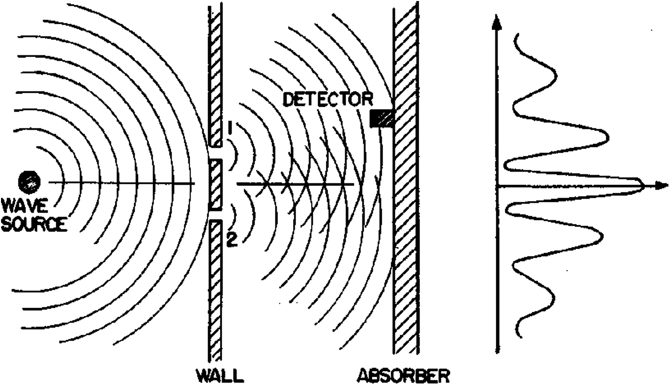
Figure 1.19. A square with sides
 and
and
 (
( ) around which the circulation of a
vector
) around which the circulation of a
vector  is calculated. The sides parallel to
the x-axis are numbered 1 and 3, while the sides parallel to the
y-axis are numbered 2 and 4.
is calculated. The sides parallel to
the x-axis are numbered 1 and 3, while the sides parallel to the
y-axis are numbered 2 and 4.
Download figure:
Standard image High-resolution image
The application of the divergence theorem to the surface integrals appearing in Maxwell's equations (1.29) and (1.31) allows these equations to be expressed in differential form. Introducing the charge density ρ associated with the charge in volume V,

equation (1.29) becomes

and thus, V being a generic volume,

Similarly one obtains
for 

In the same way, the application of the curl theorem to the line integrals of
 and
and
 in equations (1.30) and (1.32), respectively, leads to


These two equations imply that variations in time of one of the two fields produce 'rotational' configurations of the other in planes which are orthogonal to the field which generates them.
1.6.2. Electromagnetic waves
We can now show that Maxwell's equations establish that the dependence on time and
space of the electric and the magnetic fields is wave-like [5]. Without loss of generality, we consider
a simple case where the direction of propagation and the two fields
 and
and
 are mutually orthogonal:

According to this choice, equation (1.39) gives

In the same way, from equation (1.40) one obtains

Equations (1.41), (1.42) and (1.43) suggest that if one of the two fields varies in space the other varies in time, with the two fields remaining orthogonal to each other. The undulatory behaviour of the two fields can be verified by deriving equation (1.42) with respect to the spatial variable x,

where one has taken into account that the order in which the derivatives with respect to different variables are performed is irrelevant. By substituting equation (1.43) in equation (1.44) we have

This is exactly the
wave equation (1.25), with the constant factor
 correctly having the dimension of the
inverse of the square of a velocity. We can thus put
correctly having the dimension of the
inverse of the square of a velocity. We can thus put

so that equation (1.45) takes the form

On the other hand, combining the two equations obtained by deriving equation (1.43) with respect to x and equation (1.42) with respect to t, we similarly obtain for the magnetic field

Equations (1.47) and (1.48) imply that
the solutions E and B of Maxwell's equations both
satisfy the D'Alembert equation. It is thus confirmed that the two fields have
wave-like behaviour. Together they constitute the so-called electromagnetic wave,
propagating in a vacuum with a speed which does not depend on its frequency and
wavelength. Its magnitude can be calculated by substituting the numerical values of
the constants
 and
and
 in equation (1.46). We obtain

It is significant that
the velocity of propagation of the electromagnetic waves is expressed in terms of the
two fundamental constants,
 and
and
 , appearing in the description of electric
and magnetic phenomena, respectively. Its numerical value, as given in equation (1.49), is exactly
equal to the speed of light in a vacuum, thus confirming that the light is an
electromagnetic wave.
, appearing in the description of electric
and magnetic phenomena, respectively. Its numerical value, as given in equation (1.49), is exactly
equal to the speed of light in a vacuum, thus confirming that the light is an
electromagnetic wave.
References
- [1]Galilei G 2001 Dialogue Concerning the Two Chief World Systems, Ptolemaic and Copernican (New York: Modern Library)
- [2]Laplace P S 1995 A Philosophical Essay On Probabilities (: New York: Dover)
- [3]For a thorough presentation of the laws and applications of mechanics see, for example, Resnick R, Halliday D and Krane K S 2001 Physics vol 1 (New York: Wiley)
- [4]Resnick R 1968 Introduction to Special Relativity (New York: Wiley)
- [5]Halliday D, Resnick R and Krane K S 2001 Physics vol 2 (New York: Wiley)
- [6]Jackson J D 1998 Classical Electrodynamics (New York: Wiley)
- [7]Feynman R, Leighton R and Sands M 2011 The Feynman Lectures on Physics vol II (New York: Basic Books)