The normal Hall effect

The experimental study of the influence of an applied magnetic field on the electrical properties of a material dates back to the 1850s when Lord Kelvin investigated changes of the resistance of a material by the application of a magnetic field. This behavior is now known as magnetoresistance. In the 1870s Edwin Hall tried to determine if the force exerted on a conductor carrying a current by an applied magnetic field acted on the conductor as a whole or only on the charge carriers in the conductor. His observation of an electric potential normal to the flow of current is now called the Hall effect. While the phenomena of magnetoresistance and the Hall effect can be described in terms of the classical behavior of charge carriers in a solid, more recently, quantum mechanical manifestations of these behaviors have been observed. Specifically, giant magnetoresistance (GMR), and later colossal magnetoresistance (CMR) and extraordinary magnetoresistance (EMR) have been discovered. These show an effect that can be more than 10⁵ times as large as the conventional magnetoresistance. Under specific conditions, at low temperatures and in large applied magnetic fields, quantized Hall effect behavior has also been observed. In part I of the present volume, these quantum effects are contrasted to the well known classical behavior that has been observed for the electrical properties of solids in externally applied fields. In this chapter, we begin with an overview of these classical effects.

The electrical conductivity of a material can be considered for a sample with geometry, as shown in figure 1.1. Here, the length, x₀, is much greater than the width, y₀, which is much greater than the thickness, z₀. An electric field is applied along the x-direction by closing a switch connected to a voltage source. This voltage creates an electric field

$$\begin{eqnarray}&&{E}_{x}=\frac{{V}_{x}}{{x}_{0}}\end{eqnarray} \tag{ 1.1 }$$

along the x-direction. For the present, we will consider that the current in the sample may be represented by the flow of electrons as shown in the figure. The acceleration, a_x , of the electrons in response to the applied electric field will be

$$\begin{eqnarray}&&{a}_{x}=-\frac{e{E}_{x}}{{m}_{e}}=-\frac{e{V}_{x}}{{m}_{e}{x}_{0}}\end{eqnarray} \tag{ 1.2 }$$

where m_e is the mass of the electron. A time t after the switch is closed, the velocity of the electrons will be

$$\begin{eqnarray}&&{v}_{x}=-\frac{e{E}_{x}}{{m}_{e}}t\end{eqnarray} \tag{ 1.3 }$$

Current is defined as the charge transported per unit time and may be written as

$$\begin{eqnarray}&&{I}_{x}=-e{n}_{e}{v}_{x}A\end{eqnarray} \tag{ 1.4 }$$

where A is the cross sectional area of the sample normal to the current flow, i.e. A = y₀ z₀. The current density, j_x , is defined as

$$\begin{eqnarray}&&{j}_{x}=\frac{{I}_{x}}{A}=-e{n}_{e}{v}_{x}\end{eqnarray} \tag{ 1.5 }$$

and this equation can be combined with equations (1.3) and (1.4) to give

$$\begin{eqnarray}&&{E}_{x}=\frac{{m}_{e}}{{e}^{2}{n}_{e}{\tau }_{e}}{j}_{x}\end{eqnarray} \tag{ 1.6 }$$

It is customary to assume that the mean free time of the charge carriers, τ_e , is limited by scattering from other charges and phonons in the material giving

$$\begin{eqnarray}&&{E}_{x}=\frac{{j}_{x}}{{\sigma }_{e}}={\rho }_{e}{j}_{x}\end{eqnarray} \tag{ 1.7 }$$

where the conductivity, σ_e , resulting from the current carried by the electrons is defined as

$$\begin{eqnarray}&&{\sigma }_{e}=\frac{{e}^{2}{n}_{e}{\tau }_{e}}{{m}_{e}}\end{eqnarray} \tag{ 1.8 }$$

and the resistivity is defined as

$$\begin{eqnarray}&&{\rho }_{e}=\frac{1}{{\sigma }_{e}}=\frac{{m}_{e}}{{e}^{2}{n}_{e}{\tau }_{e}}\end{eqnarray} \tag{ 1.9 }$$

Equation (1.7) is the intrinsic form of Ohm's law, V = IR, which depends only on material properties, and not on sample dimensions.

Zoom In Zoom Out Reset image size

Now consider an experiment where a magnetic field, B, is applied along the z-direction. The electrons flowing through the material will experience a Lorentz force

$$\begin{eqnarray}&&\vec{F}=-e\left[\vec{E}+\vec{v}\times \vec{B}\right]\end{eqnarray} \tag{ 1.10 }$$

The magnetic field, B, sometimes called the magnetic induction, is related to the magnetic field strength, H, and the magnetization, M, as

$$\begin{eqnarray}&&B={\mu }_{0}\left(H+M\right)\end{eqnarray} \tag{ 1.11 }$$

In the case where a material has no magnetization, B and H are the same except for a numerical factor, the permeability of free space, μ₀.

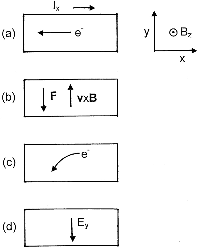
The above situation is illustrated by the geometry shown in figure 1.2. The applied electric field is in the x-direction, E_x and this causes a current to flow in the x-direction, which is comprised of negatively charged electrons traveling in the negative x-direction as illustrated in figure 1.3(a). The Lorentz force on these electrons as given by equation (1.10) is shown in figure 1.3(b), where the cross product is a vector pointing in the y-direction and the force on the electrons (because of their negative charge) is in the negative y-direction. This force will cause the electrons to be deflected, as shown in figure 1.3(c). Because there can be no net flow of current out of the sample in the y-direction, there must be a force acting on the electrons to prevent them from moving continually in this direction. This force is provided by an electric field that is established in the negative y-direction to counteract the electron flow from the Lorentz force, as shown in figure 1.3(d). One way of looking at this is to realize that if electrons flow in the negative y-direction, then this will represent a redistribution of charge in the sample and will give rise to an electric field which will oppose this flow.

Zoom In Zoom Out Reset image size

Zoom In Zoom Out Reset image size

The above situation can be expressed mathematically by writing down the y-component of the Lorentz force from equation (1.10) as

$$\begin{eqnarray}&&{F}_{y}=-e(-{E}_{y}+{v}_{x}{B}_{z})\end{eqnarray} \tag{ 1.12 }$$

The reason for the minus sign in front of the E_y term can easily be seen by an examination of the directions illustrated in figure 1.3. Since, in equilibrium, the net force in the y-direction must be zero, equation (1.12) gives the electric field in the y-direction as

$$\begin{eqnarray}&&{E}_{y}={v}_{x}{B}_{z}\end{eqnarray} \tag{ 1.13 }$$

From equation (1.3) we can write the x-component of the equilibrium velocity in terms of the electron mean free time as

$$\begin{eqnarray}&&{v}_{x}=-\frac{e{E}_{x}{\tau }_{e}}{{m}_{e}}\end{eqnarray} \tag{ 1.14 }$$

Combining equation (1.13) with equation (1.14) gives

$$\begin{eqnarray}&&{E}_{y}=-\frac{e{E}_{x}{B}_{z}{\tau }_{e}}{{m}_{e}}\end{eqnarray} \tag{ 1.15 }$$

Combining equations (1.5) and (1.14) gives the current density as

$$\begin{eqnarray}&&{j}_{x}=\frac{{e}^{2}{n}_{e}{E}_{x}{\tau }_{e}}{{m}_{e}}\end{eqnarray} \tag{ 1.16 }$$

Solving equation (1.16) for eE_x τ_e /m_e and substituting into equation (1.15) gives

$$\begin{eqnarray}&&{E}_{y}={R}_{{\rm{H}}}{B}_{z}\,{j}_{x}\end{eqnarray} \tag{ 1.17 }$$

where R_H is the Hall coefficient which is defined as

$$\begin{eqnarray}&&{R}_{{\rm{H}}}=-\frac{1}{e{n}_{e}}=\frac{{E}_{y}}{{j}_{x}{B}_{z}}\end{eqnarray} \tag{ 1.18 }$$

The Hall resistivity, R_xy , that is the resistance measured in the y-direction when the current is in the x-direction, is written as

$$\begin{eqnarray}&&{R}_{xy}=\frac{{V}_{y}}{{I}_{x}}=\frac{{E}_{y}}{{j}_{x}{z}_{0}}\end{eqnarray} \tag{ 1.19 }$$

This resistance is in contrast to the normal (or longitudinal) resistance, R_xx = V_x /I_x , which is the resistance in the x-direction when the current is in the x-direction. There is sometimes some ambiguity about the terminology used for the Hall resistance. It is sometimes referred to as R_H, which can be confused with the terminology for the Hall coefficient. It is sometimes referred to as ρ_H or ρ_xy , which suggests that it is a resistivity (although in two dimensions resistance has the same dimensions as resistivity in three dimensions). We, therefore, adopt the terminology as in equation (1.19) to avoid confusion.

The experimental measurement of the Hall coefficient provides three pieces of very important information about the electrical properties of the material;

• (1)  
  The sign of the charge carriers, in this case negative, because they were assumed to be electrons.
• (2)  
  The charge per charge carrier, assumed to be one unit of electronic charge in the above.
• (3)  
  The number density of charge carriers.

The experimental measurement of the Hall coefficient follows from a consideration of the right-hand side of equation (1.18). The electric field in the y-direction can be written in terms of the potential difference across the sample in the y-direction, V_y , as

$$\begin{eqnarray}&&{E}_{y}=\frac{{V}_{y}}{{y}_{0}}\end{eqnarray} \tag{ 1.20 }$$

and the current density in the x-direction follows from equation (1.5) as

$$\begin{eqnarray}&&{j}_{x}=\frac{{I}_{x}}{{y}_{0}{z}_{0}}\end{eqnarray} \tag{ 1.21 }$$

These two equations give

$$\begin{eqnarray}&&{R}_{{\rm{H}}}=\frac{{V}_{y}{z}_{0}}{{I}_{x}{B}_{z}}\end{eqnarray} \tag{ 1.22 }$$

The quantities on the right-hand side of equation (1.21) are all readily measurable as illustrated by the sample geometry in figure 1.1 and by the experimental schematic shown in figure 1.2. It is important not to extract current along the y-direction in the sample during the measurement of the potential difference across the sample, so a high input impedance voltmeter should be used.

A simple picture of electrical conduction in metals would suggest that the current is carried by electrons in the conduction band with a charge of one fundamental unit of electronic charge. The number density of charge carriers can be estimated on the basis of the assumed atomic valence state and the atomic density. Some results of Hall coefficients, as calculated by equation (1.18) (i.e. −1/en_e ), and experimental values, as determined by Hall voltage measurements according to equation (1.21), for some 'simple' monovalent metals are shown in table 1.1. The experimental results are in reasonable agreement with calculated values. They certainly show the proper sign for the electron charge and are consistent with a single electron per atom contributing to the conduction. However, Hall voltage measurements are subject to a number of uncertainties due to the experimental method and more accurate measurements of the Hall coefficient by methods such as helicon wave techniques yield results that are typically in much closer agreement with the calculated values. This result shows, at least for the materials in the table, that the assumptions used for the calculation of the Hall coefficient are quite reasonable.

The discussion in the previous section shows that a simple approach that deals with charge carriers as free electrons in metals provides a good description of the results obtained from Hall effect measurements. We know, however, that this simple approach is not suitable for all materials. There are two factors that this approach does not consider; firstly, that electrons, even in a metal, are not necessarily free and are constrained by the details of the band structure of the material and, secondly, in some materials, notably some semiconductors, the current can also be carried by holes. The derivation in the previous section can be repeated by assuming that the charge carriers are positively charged holes rather than negatively charged electrons. In the case of holes, the charge will be +e (rather than −e) and the number density, mass and mean free time will have values appropriate for the hole carriers, n_h , m_h and τ_h , respectively. This leads to a Hall field, analogous to equation (1.15), of

$$\begin{eqnarray}&&{E}_{y}=\frac{e{E}_{x}{B}_{z}{\tau }_{h}}{{m}_{h}}\end{eqnarray} \tag{ 1.23 }$$

and a Hall coefficient, analogous to equation (1.18), of

$$\begin{eqnarray}&&{R}_{{\rm{H}}}=\frac{1}{e{n}_{eh}}=\frac{{E}_{y}}{{j}_{x}{B}_{z}}\end{eqnarray} \tag{ 1.24 }$$

Measurements of normal resistivity or conductivity cannot distinguish between currents carried by electrons moving in one direction and currents carried by holes moving in the other direction. However, a simple measurement of the Hall voltage can readily tell the difference between these two situations. The change of sign of the Hall coefficient is reflected, from an experimental standpoint, by a change in the sign of the Hall field and, hence, the Hall voltage.

Experimental studies of p-type semiconductors, as opposed to n-type semiconductors, clearly show positive Hall coefficients indicative of the existence of hole states carrying the current. Hall effect measurements also show some surprising, and highly informative, results for some metals that are clearly related to band structure effects. Table 1.2 gives the calculated and measured Hall coefficients for some 'not-so-simple' metals. The electronic structure of aluminum is [Ne]3s²3p and for indium it is [Kr]5s²5p. Thus, in a simple model, we would expect one conduction electron per atom for both Al and In as a result of the unpaired outer p electron. However, both Al and In show a positive Hall coefficient with a value consistent with one hole carrier per atom. This situation is the result of overlapping bands giving rise to the formation of hole states.

Above absolute zero temperature we expect that all semiconducting materials will have both electrons and holes present. The majority carriers, which are the result of impurities, as well as thermal excitations, are the dominant carriers, and the minority carriers, which are thermally excited, occurs with a lower density. In the case where both electron and hole carriers are present, a thorough evaluation of the Hall coefficient requires a more detailed treatment rather than merely adding the negative (for electrons) and positive (for holes) contributions from equations (1.18) and (1.24) to the coefficient. This is because the relative contribution from each charge carrier to the total Hall field is related to its ability to respond to the applied magnetic field and this involves carrier specific characteristics, such as mass and mean free time. The question of mass will be discussed further in the next section, but for present we will consider values of m_e and m_h for the electron and hole, as was used above. These factors, which appear, for example in equation (1.16), can be taken into account by introducing the carrier mobility, which is defined for electrons and holes as

$$\begin{eqnarray}&&{\mu }_{e}=\frac{e{\tau }_{e}}{{m}_{e}}\end{eqnarray} \tag{ 1.25 }$$

and

$$\begin{eqnarray}&&{\mu }_{h}=\frac{e{\tau }_{h}}{{m}_{h}}\end{eqnarray} \tag{ 1.26 }$$

for the electrons and holes, respectively. Including both electron and hole carriers in the derivation of the Hall coefficient yields the result

$$\begin{eqnarray}&&{R}_{{\rm{H}}}=\frac{{n}_{h}{{\mu }_{h}}^{2}-{n}_{e}{{\mu }_{e}}^{2}}{e{({n}_{h}{\mu }_{h}+{n}_{e}{\mu }_{e})}^{2}}\end{eqnarray} \tag{ 1.27 }$$

Since the mobilities are related to mass, as in equations (1.25) and (1.26), it is important to consider the meaning of carrier mass in detail.

Although the mass of the charge carrier does not appear explicitly in the expressions for the Hall coefficients, equations (1.18) and (1.24), it is an important parameter in the description of charge transport in solids. For example, mass appears explicitly through the mobilities in equation (1.27) for systems in which both carrier polarities are present. It is also an important factor in the description of electron behavior in the presence of very high magnetic fields. In the case illustrated in figure 1.2 where there is no electric field in the x-direction and the magnetic field is sufficiently high, then the electrons will assume circular orbits in the material. This will be an important feature of the quantum Hall effect described below. In this case, the Lorentz force given by equation (1.12) with E_y = 0, can be set equal to the centripetal acceleration of the electron in a circular orbit of radius r;

$$\begin{eqnarray}&&evB=\frac{{m}_{e}{v}^{2}}{r}\end{eqnarray} \tag{ 1.28 }$$

The angular frequency of the electron in the orbit is related to its velocity by

$$\begin{eqnarray}&&\omega =\frac{v}{r}\end{eqnarray} \tag{ 1.29 }$$

Equations (1.28) and (1.29) can be combined to yield the angular frequency as

$$\begin{eqnarray}&&\omega =\frac{eB}{{m}_{e}}\end{eqnarray} \tag{ 1.30 }$$

This frequency is known as the cyclotron frequency.

Although it may be unclear what the mass of the hole is, one might expect that the mass of the electron which has appeared in the equations above is the mass of a free electron. This is not the case for an electron in a solid as the behavior of the electron is governed by the band structure of the material. The mass in the above discussion is, therefore, not the free particle mass but an effective mass that appears in the equations of motion. Let us look at a simple one-dimensional example.

The dispersion relation for free electrons relates the energy, E, to the momentum, p (or equivalently wave vector, k), by the relationship

$$\begin{eqnarray}&&E=\frac{{p}^{2}}{2m}=\frac{{\hslash }^{2}{k}^{2}}{2m}\end{eqnarray} \tag{ 1.31 }$$

Taking the second derivative of this expression gives

$$\begin{eqnarray}&&\frac{{\partial }^{2}E}{\partial {k}^{2}}=\frac{{\hslash }^{2}}{m}\end{eqnarray} \tag{ 1.32 }$$

from which the inverse mass may be defined as

$$\begin{eqnarray}&&\frac{1}{m}=\frac{1}{{\hslash }^{2}}\frac{{\partial }^{2}E}{\partial {k}^{2}}\end{eqnarray} \tag{ 1.33 }$$

If this approach is extended to electrons which are not free electrons (i.e. they are on bands which are not parabolic) then the mass in equation (1.33) is the effective mass, m*;

$$\begin{eqnarray}&&\frac{1}{m* }=\frac{1}{{\hslash }^{2}}\frac{{\partial }^{2}E}{\partial {k}^{2}}\end{eqnarray} \tag{ 1.34 }$$

If this picture is extended to three dimensions, then we find that the effective mass can be (and usually is) different in different directions. This is obvious because the shape of the bands (that is the energy as a function of wave vector) is different in different directions and thus, the second derivative in equation (1.34) will be different in different directions. It is, therefore, necessary in a full treatment of this problem, to express mass as a tensor. This tensor will include terms representing (for example) the response of a particle in the x-direction to a force exerted in the x-direction but can also include terms representing the response of a particle in the x-directions to a force exerted in the y-direction. We can consider a simple two-dimensional classical analog of this situation to clarify this concept.

Consider a mass, m, on a frictionless inclined plane at an angle of θ with respect to the x-axis as illustrated in figure 1.4. To simplify the analysis the effect of gravity will be ignored. If an external force is applied in the x-direction to the mass as shown in figure 1.4(a) then the acceleration of the mass will be as illustrated. The movement of the mass is constrained by its interaction with the surface of the plane, just as the movement of electrons (or holes) in a solid is constrained by the features of the band structure. The acceleration as illustrated in figure 1.4(a) has both x- and y-components which may be written as

$$\begin{eqnarray}&&{a}_{xx}=\frac{{F}_{x}}{m}{\cos }^{2}\,\theta \end{eqnarray} \tag{ 1.35 }$$

and

$$\begin{eqnarray}&&{a}_{yx}=\frac{{F}_{x}}{m}\,\sin \,\theta \,\cos \,\theta \end{eqnarray} \tag{ 1.36 }$$

where a_ij represents the acceleration in the i-direction as a result of a force in the j-direction. For figure 1.4(b) the force is along the y-axis and the accelerations will be

$$\begin{eqnarray}&&{a}_{xy}=\frac{{F}_{y}}{m}\,\sin \,\theta \,\cos \,\theta \end{eqnarray} \tag{ 1.37 }$$

and

$$\begin{eqnarray}&&{a}_{yy}=\frac{{F}_{y}}{m}{\sin }^{2}\,\theta \end{eqnarray} \tag{ 1.38 }$$

Zoom In Zoom Out Reset image size

On the basis of equations (1.35) to (1.38) the simple scalar form of Newton's law, a = F/m may be written as a tensor equation

$$\begin{eqnarray}&&\left(\begin{array}{c}{a}_{x}\\ {a}_{y}\end{array}\right)=\left(\begin{array}{cc}\frac{{\cos }^{2}\,\theta }{m} & \frac{\sin \,\theta \,\cos \,\theta }{m}\\ \frac{\sin \,\theta \,\cos \,\theta }{m} & \frac{{\sin }^{2}\,\theta }{m}\end{array}\right)\left(\begin{array}{c}{F}_{x}\\ {F}_{y}\end{array}\right)\end{eqnarray} \tag{ 1.39 }$$

where the vector components of the acceleration are related to the vector components of the force by the inverse effective mass tensor. This may be written in simple component form as

$$\begin{eqnarray}&&{a}_{i}=\left(\frac{1}{m* }\right){}_{ij}F_{j}\end{eqnarray} \tag{ 1.40 }$$

This approach is analogous to the situation in three dimensions for electrons in a solid where the components of the 3 × 3 inverse effective mass tensor may be written in terms of second derivatives of the energy with respect to the spatial components of the wave vector as

$$\begin{eqnarray}&&{\left(\frac{1}{m* }\right)}_{ij}=\frac{1}{{\hslash }^{2}}\frac{{\partial }^{2}E}{\partial {k}_{i}\partial {k}_{j}}\end{eqnarray} \tag{ 1.41 }$$

All applications of the Hall effect are related to the sensitivity of the electronic transport properties of materials to the presence of an external magnetic field. In general, practical devices that make use of the Hall effect are designed with materials which will optimize the effect of magnetic fields. Devices fall basically into two categories, those designed for measurement and those designed for control.

The Hall effect is one of the simplest accurate methods of measuring magnetic fields. If a Hall effect device as illustrated in figure 1.2 is constructed from a material with a known Hall coefficient, then the magnetic field can be obtained from a measurement of the Hall voltage according to equation (1.22). Rewriting this equation to give the magnetic field, we find

$$\begin{eqnarray}&&{B}_{z}=\frac{{V}_{y}{z}_{0}}{{I}_{x}{R}_{{\rm{H}}}}\end{eqnarray} \tag{ 1.42 }$$

If the dimensions of the sample (i.e. z₀) and the current in the x-direction (i.e. I_x ), then a simple measurement of the Hall voltage will provide the magnetic field.

The ability of a Hall effect sensor to detect magnetic fields makes it useful for a number of control applications. A simple proximity detector can be constructed using a Hall sensor and a permanent magnet. If the spatial variation of the field produced by the permanent magnet is known, then the relative locations of the magnet and the Hall sensor can be determined.

A Hall sensor can be used to measure the frequency of rotation of a shaft may be measured by placing a permanent magnet on the side of the shaft. This approach can be used with a feedback circuit to control rotational frequency.

References

- Ashcroft N W and Mermin N D 1976 Solid State Physics (Boston, MA: Cengage)
- Hurd C M 1972 The Hall Effect in Metals and Alloys (New York: Plenum)
- Kittel C 2005 Introduction to Solid State Physics 8th edn (Hoboken, NJ: Wiley)