
Abstract
Temporal focusing microscopy provides the optical sectioning capability in wide-field two-photon fluorescence imaging. Here, we demonstrate temporal focusing microscopy combined with three-dimensional structured illumination, which enables us to enhance the three-dimensional spatial resolution and reject the background fluorescence. Experimentally, the periodic pattern of the illumination was produced not only in the lateral direction but also in the axial direction by the interference between three temporal focusing pulses, which were easily generated using a digital micromirror device. The lateral resolution and optical sectioning capability were successfully enhanced by factors of 1.6 and 3.6, respectively, compared with those of temporal focusing microscopy. In the two-photon fluorescence imaging of a tissue-like phantom, the out-of-focus background fluorescence and the scattered background fluorescence could also be rejected.
Export citation and abstract BibTeX RIS

Content from this work may be used under the terms of the Creative Commons Attribution 4.0 license. Any further distribution of this work must maintain attribution to the author(s) and the title of the work, journal citation and DOI.
1. Introduction
Super-resolution microscopy has become a powerful tool for investigating biological phenomena.1–11) However, there is a trade-off between the spatial resolution and penetration depth in optical imaging techniques. If the spatial resolution is enhanced by a factor of N, the signal intensity is reduced by a factor of N3 due to the decreased signal volume. The lower intensity signal is easily buried in the background fluorescence generated in the out-of-focus regions. Thus, it is difficult to use super-resolution microscopy for the deep imaging of biological tissue. In contrast, two-photon excited fluorescence (TPEF) microscopy has attractive advantages over confocal microscopy including decreased background fluorescence and deeper penetration into thick specimens.12,13) On the other hand, the spatial resolution of TPEF microscopy is lower than that of confocal microscopy utilizing visible light due to the use of near-infrared light.
Recently, super-resolution microscopy was combined with TPEF microscopy to perform deep imaging.14–19) In general, as stimulated emission depletion (STED) microscopy1,2) employs a tightly focused beam as an excitation light, it can be easily coupled with laser scanning TPEF microscopy.14,15) In contrast, structured illumination microscopy (SIM),3,4) saturated SIM,5–7) and single-molecule localization microscopy (SMLM)8–11) require a wide-field illumination scheme. Temporal focusing (TF), which provides wide-field two-photon excitation with optical sectioning capabilities,20,21) allows SIM17) and SMLM16) to operate in deep imaging. In a wide-field microscope, the fluorescent photons generated in the focal plane must be imaged in their conjugate positions on a two-dimensional (2D) detector. Thus, if the emitted photons are scattered within the sample, the scattered photons become the background fluorescence. This problem has been solved by applying non-super-resolution SIM, which enables the rejection of the scattered background fluorescence,22) to TF microscopy.17,23) To obtain a large field-of-view, the excitation power must be increased. As TF microscopy does not require laser scanning, it can utilize an amplifier, which operates at low repetition rates (lower than megahertz), as an excitation light source. Therefore, by using amplified pulses at a low average power, TPEF video-rate imaging over large areas in the 5000–20000 µm2 range has been achieved.24,25) By using the time multiplexing technique,26,27) the out-of-focus background fluorescence generated in the TF microscope has been suppressed.28,29) The multifocal TPEF technique30,31) can also be combined with SIM.18,19) However, in multifocal SIM, multiple foci must be scanned. Thus, to increase the imaging speed, the repetition rate of the pulses must be more than several tens of megahertz.
Since the spatial resolution of super-resolution SIM is enhanced in the periodic pattern direction, a periodic illumination pattern in the axial direction as well as the lateral direction allows the enhancement of the spatial resolution in both the axial and lateral directions.32) However, in TF microscopy combined with super-resolution SIM ever reported, only laterally structured illumination, which is produced by the interference between two TF pulses, has been used.17) In this paper, we demonstrate three-dimensional (3D) interferometric TF (ITF) microscopy in which periodic patterns are generated in the lateral and axial directions by the interference between three TF pulses. The three TF pulses is generated by employing a digital micromirror device (DMD), which can be utilized both as a phase grating to generate TF pulses33) and an amplitude grating to achieve 3D structured illumination.34) Thus, the use of DMD can also enable us to simplify a complex ITF microscope, which includes a grating for TF and a beamsplitter or another grating for structured illumination.17) TF microscopy combined with SIM using the DMD has already been reported.35) But the 3D structured illumination has been treated incorrectly as a 2D periodic pattern only in the lateral direction. The required pattern images for 3D structured illumination is different from that for 2D structured illumination. In Sect. 2, we start with an explanation of the concept of 3D-ITF microscopy and show an experimental setup for it. In Sect. 3, we report and discuss the experimental results of 3D-ITF microscopy. In Sect. 4, we summarize this paper.
2. Methods
2.1. Theory
We first show the principle of 3D-ITF microscopy. As shown in Fig. 1, in TF microscopy, all the spectral components in a spectrally dispersed pulse are recombined only at the focal plane of an objective lens. As a result, the pulse duration decreases as the distance from the focal plane decreases and becomes the shortest at the focal plane. Thus, although the wide field illumination is used, the TF effect provides the suppression of the out-of-focus TPEF. The focal plane is imaged onto a 2D detector, which is used to record a wide-field image. A 3D image is obtained by scanning the sample along the axial direction. Therefore, the detected image D ( ) can be expressed as

where  is the density distribution of the fluorophore in the sample,
  is the time-averaged intensity distribution of a TF pulse, and
  is the point spread function (PSF) of the detection system. ATF(z) is the axial response for two-photon excitation by the TF pulse, which is described by36,37)

Here, zR is related to the optical sectioning capability by the TF effect, which depends on the numerical aperture. We assume that the sample is illuminated by an excitation light with a periodic pattern, which is generated by the interference of three TF pulses, as shown in Fig. 1. If we represent the time-averaged electric field of the excitation light as

the square of the time-averaged intensity can be written as

where

Here, α is a modulation depth, k0 is the wavevector of the pulse center wavelength, θ is the angle between the central and outer beams, and ϕm is the phase shift of the periodic pattern. By using Eqs. (1) and (4), the detected image can be rewritten as

where  denotes a convolution. The detected image in Fourier space is given by

where

As shown in Eq. (7), the detected image includes nine Fourier components,  , at spatial frequencies of around −4ky0, −3ky0, −2ky0, −ky0, 0, +ky0, +2ky0, +3ky0, and +4ky0 in the ky-direction. In each Fourier component, the high spatial frequency sample information
  is down-converted to the lower frequency information
  in the ky-direction. In addition, the detectable bandwidth in the kz-direction is broadened by the convolution of the optical transfer function (OTF) of the detection system with the excitation effects of the TF and the periodic pattern illumination along the axial (z) direction. By shifting the down-converted components
  back to their true positions
  in Fourier space and by recombining them, the effective OTF of the microscope is broadened.38) As a result, the cut-off spatial frequencies in the ky and kz-directions are extended to kyd + 4ky0 and kzd + kTF + 2kz0, respectively. Here, kyd and kzd are the cut-off spatial frequencies of the detection system OTF in the ky- and kz-directions, and kTF is the cut-off spatial frequency of the TF effect. Thus, in order to reconstruct the super-resolution images, each Fourier component
  must be separated. To separate each Fourier component, we take nine images,
  , at phase shifts ϕm = ϕ0 + mϕs from m = 0 to 8, and use the principle of homodyne detection:

Here the phase step ϕs is 2π/9, and ϕ0 is the offset phase. After shifting the separated Fourier components back to their true position, they are recombined with the exception of the Fourier component at the spatial frequency of around 0,  . As the scattered background fluorescence and the out-of-focus background fluorescence do not produce the periodic pattern on the 2D detector, they are contained in
  .17) Thus, to reject the background fluorescence,
  is not used. The super-resolution image can be acquired by the inverse Fourier transform of the recombined image in Fourier space. In order to enhance the spatial resolution in 3D, the orientation of the periodic pattern must be rotated in the lateral direction.

Fig. 1. Schematics for the 3D-ITF technique.
Download figure:
Standard image High-resolution image2.2. Experimental setup
Figure 2(a) shows a schematic diagram of the system used for 3D-ITF microscopy. As an excitation light source, an Yb-fiber chirped-pulse amplifier (CPA) was utilized. The output pulse from an Yb-fiber oscillator (Onefive Origami-10), which produced 152 fs pulses at a central wavelength of 1061 nm, a bandwidth of 8.1 nm, and a repetition rate of 40 MHz, was used as a seed pulse. In the CPA, the input pulse with an average power of 15 mW was stretched to 203 ps using a fiber stretcher with a group delay dispersion (GDD) of 7.5 ps2 and a third order dispersion (TOD) of −0.087 ps3. The output spectrum from the stretched fiber was broadened to the bandwidth of 19 nm by self-phase modulation. The stretched pulse was amplified to an average power of 330 mW by the first Yb-fiber amplifier. After the first amplification, the repetition rate was reduced to 200 kHz by using an acousto-optic modulator (AOM). The output pulse from the AOM was amplified to an average power of 252 mW by a second Yb-fiber amplifier. The amplified pulse was compressed using the combination of a pulse shaper with a liquid-crystal spatial light modulator (SLM) and a pair of 1600 lines/mm transmission gratings with a separation of 12 cm at an incident angle of 59.1°. The pulse shaper was used to compensate for the higher-order dispersion of the system, while the grating pair was used for the simultaneous GDD and TOD compensation. The output pulse from the CPA was reflected by a DMD (Texas Instruments DLP4500NIR) with a micromirror pitch of 10.8 µm and a micromirror tilt angle of ±12°. As shown in Fig. 2(b), the DMD can operate both as an amplitude grating and as a phase grating. In the x-direction, all the micromirrors on the DMD were tilted by +12° or −12°, which indicated on or off states, respectively. As the tilt angle of the micromirror on the DMD is regarded as the blaze angle of a blazed grating along the x-direction, the spectrally dispersed pulse for the TF was generated using the DMD as the phase grating. To avoid the tilt of the TF plane on the sample, the diffraction angle of the central wavelength must be zero. Considering the blaze condition to maximize the diffraction efficiency, we chose a fourth order diffraction light at an angle of incidence of 23.1°. Under this condition, the diffraction efficiency was 54%. Conversely, in the y-direction, the periodic pattern with on and off states were produced at a period of 18 micromirrors. The periodic pattern was utilized as an amplitude grating along the y-direction, which gave zero and ±1 order diffraction lights as three TF pulses. The periodic pattern on the DMD was imaged at the focal plane of a water-immersion objective lens with a numerical aperture (NA) of 1.2 (OB; Olympus UPLSAPO60×W) by a factor of 1/125×. The periodic pattern near the focal plane was observed not only in the lateral direction but also in the axial direction. By blocking the zero-order diffraction beam, the periodic pattern was only produced in the lateral direction. The pulse duration at the focal plane was 103 fs and the input power was 9 mW on the sample surface. The generated TPEF signal was collected by the same objective lens and was separated from the excitation pulses using a dichroic mirror (DM; Thorlabs DMLP900). To remove the residual excitation pulses, a short-pass filter (SPF; Semrock FF01-890/SP-25) and a bandpass filter (BPF; Semrock FF01-550/88-25) were used. Wide-field TPEF images were obtained by a CMOS camera (Hamamatsu Photonics ORCA-Flash2.8) with an exposure time of 10 ms. In order to achieve the resolution enhancement in all the lateral directions, the orientation of the periodic pattern on the DMD was rotated by 45, 90, and 135°. By scanning the sample in the axial (z) direction with a stepping motor-driven stage with a step size of 100 nm, the 3D image was obtained. By replacing the DMD with a reflective diffraction grating with a groove density of 830 grooves/mm, TPEF images for the TF microscope were acquired.

Download figure:
Standard image High-resolution image
Fig. 2. 3D-ITF microscope setup. SLM: spatial light modulator, DM: dichroic mirror, OB: objective lens, SPF: short-pass filter, BPF: bandpass filter.
Download figure:
Standard image High-resolution image3. Results and discussion
In order to obtain the fundamental spatial frequency of the periodic pattern ky0, a TPEF image of the Rhodamine B solution was recorded under a structured illumination. From the measured fringe pattern, the fundamental spatial frequency of the periodic pattern in the lateral direction, ky0, was evaluated to be 4.1 rad/µm, which was used to reconstruct the 3D-ITF image. The signal-to-noise ratios of the Fourier components,  , at the spatial frequencies of around −4ky0 and +4ky0 were too low to be used in the reconstruction of the 3D-ITF image.
We characterized the optical sectioning capability of 3D-ITF microscopy. Figure 3 shows the measured signal intensity distribution along the axial direction near the interface between the coverslip and the Rhodamine B solution. The full width at half maxima (FWHMs) of the smoothed first derivatives of the signal distributions for TF and 3D-ITF microscopies were 2.6 and 0.72 µm, respectively. We found that the optical sectioning capability of 3D-ITF microscopy was 3.6 times higher than that of TF microscopy. Compared with the optical sectioning capability of 2D-ITF microscopy with the periodic pattern illumination only in the lateral direction, which was reported to be 0.89 µm,17) that of 3D-ITF microscopy was also enhanced by a factor of 1.2. This improvement is due to the periodic pattern illumination along the axial direction.

Fig. 3. TPEF signal distributions along the axial direction near the interface between the coverslip and the Rhodamine B solution, which were acquired by TF (○) and 3D-ITF (×) microscopies, and their smoothed first derivatives for TF (dashed line) and 3D-ITF (dotted line) microscopies.
Download figure:
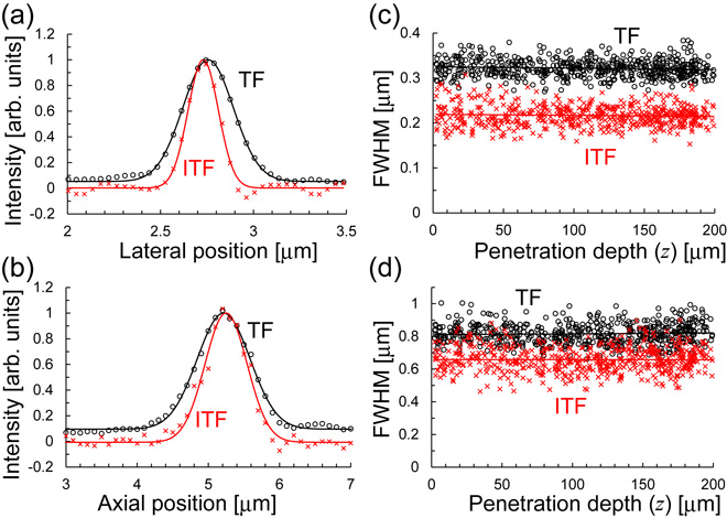
Standard image High-resolution imageIn order to investigate the spatial resolution of 3D-ITF microscopy, we obtained a 3D image of 200-nm fluorescent polystyrene beads (Molecular Probes F8809) with a concentration of 2.3 × 10¹¹ beads/mL in a low-melting-point agarose gel. The emission wavelength of the beads was 560 nm. The 3D images were reconstructed from 2001 cross-sectional ITF or TF images. By extracting the 1D signal distribution of a bead along the lateral and axial directions, as shown in Figs. 4(a) and 4(b), and by fitting each distribution with Gaussian functions, the FWHMs in the lateral and axial directions were acquired. Figures 4(c) and 4(d) illustrate the FWHMs in the lateral and axial directions at various penetration depths, respectively. The lateral FWHMs for TF and 3D-ITF microscopies were evaluated to be 0.32 ± 0.015 and 0.22 ± 0.018 µm, respectively. The lateral FWHM of the fluorophore distribution in a 200-nm bead was 0.173 µm, which is close to the measured lateral FWHM. Thus, we estimated the lateral FWHMs of the effective PSFs for TF and 3D-ITF microscopies, which were obtained by the numerical deconvolution of the Gaussian functions at FWHMs of 0.32 and 0.22 µm with the fluorophore distribution in a 200-nm bead, to be 0.30 and 0.18 µm, respectively. The axial FWHMs for TF and 3D-ITF microscopies were 0.82 ± 0.050 and 0.66 ± 0.059 µm, respectively. We found that the FWHMs in the lateral and axial directions were enhanced by factors of 1.6 and 1.2, respectively. For the diffraction-limited detection system at a wavelength of 560 nm and an NA of 1.2, the cut-off spatial frequencies of the OTF in the lateral and axial directions, kyd and kzd, were theoretically calculated to be 26.9 and 8.4 rad/µm, respectively. As the fundamental spatial frequency of the periodic pattern in the lateral direction, ky0, was 4.1 rad/µm, the third harmonic spatial frequency of the periodic pattern in the lateral direction, 3ky0, and the second harmonic spatial frequency of the periodic pattern in the axial direction, 2kz0, were experimentally evaluated to be 12.3 and 2.3 rad/µm, respectively. From the FWHM of 2.6 µm for the characterization of the optical sectioning capability, the cut-off spatial frequency in the axial direction by the TF effect, kTF, was evaluated to be around 2.4 (= 2π/2.6) rad/µm. Thus, the cut-off spatial frequencies of the effective OTF in the lateral and axial directions should be extended to 39.2 rad/µm (= kyd + 3ky0) and 13.2 rad/µm (= kzd + kTF + 2kz0), which results in the 0.16-µm lateral FWHM and 0.48-µm axial FWHM of the effective PSF, respectively. Compared with the minimum FWHM at the diffraction limit, the measured FWHMs are slightly broadened due to the wavefront distortion. However, the 3D spatial resolution is improved by 3D-ITF microscopy. Figure 5 illustrates the cross-sectional images at penetration depths of 45 and 162 µm. The line profiles in Fig. 5 clearly show the separation of the neighboring beads due to the improved resolution of 3D-ITF microscopy.

Fig. 4. TPEF signal distributions of a 200-nm bead at a penetration depth of 2.6 µm along the (a) lateral and (b) axial directions, which were obtained by TF (○) and 3D-ITF (×) microscopies. FWHMs in the (c) lateral and (d) axial directions at various penetration depths for TF (○) and 3D-ITF (×) microscopies.
Download figure:
Standard image High-resolution image
Fig. 5. Cross-sectional (a, c) TF and (b, d) 3D-ITF images of 200-nm fluorescent beads at penetration depths of (a, b) 45 µm and (c, d) 162 µm. The signal intensities were normalized by the maximum intensity in each image. Normalized signal profiles of TF (○) and ITF (×) microscopies along the lateral direction indicated by arrows in (e) a and b, and (f) c and d.
Download figure:
Standard image High-resolution imageUsing TF and 3D-ITF microscopy, we imaged fluorescently labeled beads in a tissue-like phantom. The phantom consisted of a low-melting-point agarose gel containing 200-nm and 2-µm fluorescent polystyrene beads at concentrations of 2.3 × 10¹¹ and 9.0 × 10⁸ beads/mL, respectively. The observed images are depicted in Fig. 6. In the image obtained by TF microscopy, the TPEF signals from the 200-nm beads are buried in the large background fluorescence, which originated from the out-of-focus TPEF of the 2-µm beads and the scattered TPEF. In contrast, the 200-nm beads are clearly visualized by 3D-ITF microscopy. The large background fluorescence could be successfully rejected by 3D-ITF microscopy.

Fig. 6. (a) 3D TF and (b) 3D-ITF images of the tissue-like phantom including 200-nm and 2-µm fluorescent beads. The signal intensities in a and b were normalized by the maximum intensity in each 3D data set. Cross-sectional (c) TF and (d) 3D-ITF images in a and b. The signal intensities in c and d were normalized by the maximum intensity in each image. (e) Normalized signal profiles of TF (○) and ITF (×) microscopies indicated by arrows in c and d.
Download figure:
Standard image High-resolution image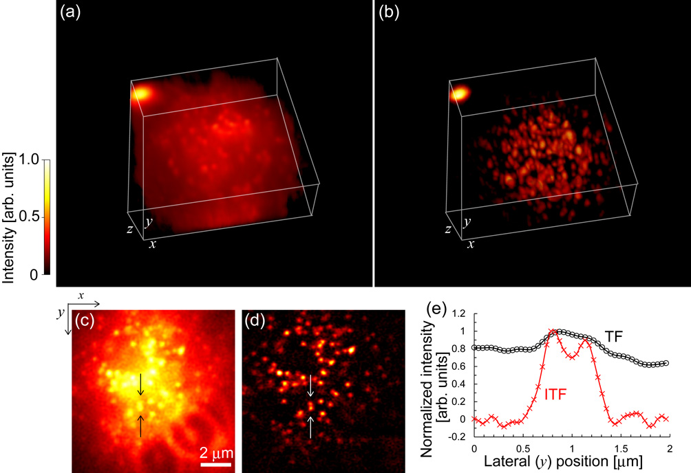
4. Conclusions
We have demonstrated that 3D-ITF microscopy combining TF microscopy with 3D structured illumination allows the improvement of 3D spatial resolution and the elimination of background fluorescence. A 3D structured illumination was achieved by the interference between three TF pulses, which were easily generated by using a DMD both as an amplitude grating and as a phase grating. The lateral and axial FWHMs of the effective PSF was enhanced by factors of 1.6 and 1.2, respectively, compared with those of TF microscopy. The optical sectioning capability was improved by a factor of 3.5. This approach can be applied to super-resolution deep imaging. The amplified pulses used in these demonstrations can be used to induce TPEF saturation. The nonlinearity of the saturation effect provides the possibility of further enhancement to the spatial resolution. By employing saturation nonlinearity in one-photon excited fluorescence (OPEF), the spatial resolution of SIM was improved.5–7) However, OPEF saturation generates large out-of-focus background fluorescence and induces photobleaching due to the high excitation intensity. TPEF and photobleaching in out-of-focus regions can be decreased by using the TF effect. In-focus photobleaching can additionally be reduced by decreasing the repetition rate of the amplified pulse to several hundreds of kilohertz.39)
Acknowledgments
We thank Dr. Yasuo Nabekawa of RIKEN for providing the spatial light modulator. One of the authors (KI) gratefully acknowledges the valuable discussions about the fiber CPA with Professor Yohei Kobayashi of the University of Tokyo and Professor Satoshi Wada of RIKEN. KI is also grateful to Dr. Yasuyuki Nakanishi of MEGAOPTO Co., Ltd. for loaning the fiber fusion splicer and for teaching him how to use it. This work was partially supported by the Research Foundation for Opto-Science and Technology and PRESTO, JST.