

Abstract
We performed time domain propagating spin-wave (SW) spectroscopy to investigate SW soliton formation. By choosing backward volume SW mode, we successfully observed a multiple solitons formation and propagation. The SW power dependence on the duration of excitation signal showed nonlinear dependence, and SW maintained its wave packet width. By making a contour plot of SW power, the evolution of SW soliton was clearly demonstrated. The generation and annihilation of SW soliton exhibited a complicated behavior, showing the competition between nonlinear effect and dispersion/relaxation effects.
Export citation and abstract BibTeX RIS
1. Introduction
Magnonics aims for ultralow power consumption devices utilizing the virtue of spin waves (SWs) in magnetic materials; the SWs generate no electric Joule heating. The SWs thus have been considered to be a promising information carrier even in a millimeter scale device chip.1–6) Due to the ultralow magnetic damping material, yttrium iron garnet (YIG), the magnonics demonstrated several device prototypes including NAND, NOR, AND, and OR logic gates.7–11)
The principle of magnonic logic operation is the phase interference by using a Mach–Zenhder-type interferometer,12) a three terminal interference device, and a ψ-shaped element.13–17) Even though single device element was proved to be applicable to magnonic logic gate, a successive signal processing has never been demonstrated. The magnonic signal transferring from single magnonic element to another is the crucial issue.18,19) Also to integrate a magnonic element up to the similar level of current CMOS devices, nanoscale fabrication technology is essential. In these recent situations, we presented the possibility of magnonic architecture using so called magnetostatic backward volume spin-wave (MSBVW) in metallic structure,20,21) since the shape magneto-anisotropy which can eliminate the application of bias magnetic field.
The MSBVW in magnetic materials has another potential to overcome problem in transferring of magnonic signals. In previous papers, the existence of magnetic soliton had been reported.22–31) The magnetic solitons was observed clearly in MSBVW mode of SWs. The magnetic soliton (spin-wave soliton) is generated by nonlinear interactions in SWs and can keep its wave packet even in a millimeter scale. If it is possible to control the nonlinear interaction for linear SWs to change into soliton, the efficiency of magnonic logic operation and succeeding transmission of output SW could be greatly improved. This means that the understanding of generation of SW soliton in magnetic materials is an important issue.
Even though the property of magnetic soliton had been widely experimented and reported,27,31) a lot of uncertainty about soliton formation is remain, especially mechanism of multiple-soliton generation did not show agreement with the theory based on nonlinear Schrödinger equation (NLSE). To intend to apply these techniques for metallic magnonic system, we revisited the generation of SW soliton and discussed the problems by using YIG systems.
In this paper, we report on the electrical detection of generation of SW soliton. The time domain propagating SW spectroscopy reveals clear wave packet in linear and nonlinear excitation power regimes. By changing a power and duration of excitation signal, we estimated a required nonlinear interaction time to generate SW soliton. By using a fast RF switch technique, we observed clear 4 SW soliton generation which agree to the prediction of nonlinear theory.
2. Experimental methods
Figure 1 shows a variable transducer structure and setup of our experimental apparatus. An YIG stripe made by the liquid phase epitaxy on garium gadrinium garnet substrate was used as a SW waveguide. The thickness and length of YIG waveguide was 5.1 μm and 21.0 mm, respectively. The width of YIG is 1.3 mm. The edge of YIG stripe was cut to have 45° angle to prevent the boundary reflections.
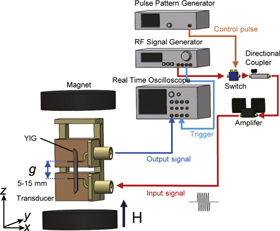
Fig. 1. (Color online) Schematic illustration of experimental. Variable transducer was imposed in an electromagnet. Fast RF switch and RF signal generator were used for excitation signals. A 3W amplifier was used to cause a nonlinear effect. A fast real-time oscilloscope was connected to one of transducer antennas to detect SW signals. On top of the antennas, a YIG waveguide was placed.
Download figure:
Standard image High-resolution imageAs shown in Fig. 1, an external magnetic field Hext was applied normal (x-direction) to the waveguide so that SWs can propagate in magnetostatic surface spin-wave (MSSW),9,16,17) and applied parallel (z-direction) to the waveguide for MSBVW.9,16,17) To make an excitation RF signal, we used a combination of fast RF switch and continuous wave generator. The fast RF switch allows a variable duration of excitation signal. By using a pulse pattern generator with 1 MHz repetition frequency, the duration T0 was changed from 5 to 150 ns. To cause nonlinear effect and to generate SW soliton, we used a 3 W amplifier and the frequency of continuous wave signal was set to be fCW = 5.8 GHz.
We used the time domain propagating SW spectroscopy.4,18) The excitation antenna generates a RF magnetic field, exciting a SW in the YIG waveguide. Excited SW propagates underneath the detection antenna which detects the SW signal by the Faraday's law of electromagnetic induction. An electric voltage VSW induced in the detection antenna was transferred into a fast real-time oscilloscope. The distance g between excitation and detection antennas was changed from 5.0 to 15.0 mm.
3. Results and discussion
3.1. Linear SW properties and dispersion relations
In Fig. 2, we showed typical waveforms of propagating SW in MSSW and MSBVW modes. To examine the linear SW transport properties, the RF amplifier was set to be ×1 amplification and the propagation distance was fixed to be g = 5 mm. In case of MSSW, the power and duration of excitation signal were set to be Pin = 3 mW and T0 = 10 ns, respectively. In case of MSBVW, the power and duration of excitation signal were Pin = 20 mW and T0 = 10 ns, respectively. Since we used fixed frequency excitation, a resonant condition was searched by detecting an external magnetic field at which the SW signals maximize their amplitude.

Fig. 2. (Color online) Time-domain waveforms (a) in MSSW modes, and (b) their power spectra obtained by the FFT analysis. The inset shows experimental f–H relation and fitting analysis. (c) The waveforms in MSBVW modes, and (b) their power spectra. The inset represents experimental f–H relation and fitting analysis. The propagation distance is fixed to be g = 5 mm.
Download figure:
Standard image High-resolution imageSW packets were clearly observed and exhibited in Fig. 2. In case of MSSW configuration, at t = 0, an excitation pulse was applied and caused an initial magnetization oscillation, inducing small signal at t = 0 less than 3 mV. The initial oscillation was induced by the direct radiation of electromagnetic wave from input antenna, resulting no time delay of excitation. The SW shows a propagating time delay and reached at detection antenna later than 35 ns, exhibiting a relatively large amplitude up to 34 mV. As increasing the external magnetic field, the velocity of SW decreases [see Fig. 2(a)] ranging in 43 < vg < 100 km s−1. The power spectra calculated by FFT analysis of time domain waveform are shown in Fig. 2(b) and they exhibit sharp peaks.
To confirm the SW mode of SW packet, we depicted the magnetic field dependence of resonant frequency f in the inset of Fig. 2(b). As shown, the experimental data are well explained by using the theoretical MSSW dispersion relations:13,32)
with the gyromagnetic ratio γ = 17.6 MHz/Oe and the film thickness d = 5.1 μm. The fitting parameters are the saturation magnetization 4πMs = 1750 G and wavenumber k = 14 600 ± 1730 m−1. While the wavenumber of excited SW can be roughly estimated by the geometry of excitation antenna  where wantenna = 50 μm is a width of antenna, the wavenumber is estimated to be 10 000 m−1 in the same order and it is plausible. The MSSW propagation was successfully demonstrated by our RF switch method.
In Fig. 2(c), we presented time domain waveforms in the MSBVW configuration. Compared to the MSSW, the amplitude of MSBVW becomes weak, approximately less than 4 mV. The MSBVW wave packets are indicated by arrows which overlapped with the tail of initial magnetization oscillation. The group velocity of MSBVW were ranging in 24 < vg < 28 km s−1. To check the SW mode, the FFT analysis was performed in Fig. 2(d), and f– H relation was shown in the inset.
The theoretical MSBVW dispersion relations20,21,32)

explains the experimental data using the parameter 6700 < k < 14 600 m−1 and 4πMs = 1750 G. Since the frequency change was smaller than MSSW, the curve fitting has a smaller dependence on the magnitude of wavevector k and did not be perfectly converged. Basically, the wavevector k is determined by the antenna geometry, however, the coupling between excitation field and MSBVW could be different from MSSW. The wavevector range may corresponds to this fact.
3.2. Lighthill criteria
The linear transport properties both in MSSW and MSBVW were well deduced by the experiments. Here, we should note that it is important to focus on the nonlinear parameter N defined by31)

where ω and u correspond to the frequency and amplitude of SW, respectively. To cause a nonlinear effect, the amplitude of SW must be tuned by experimental condition, i.e. input excitation power. According to the Lighthill criteria,33) we have to also select a SW mode which satisfies the condition

where  is the second derivative of SW frequency with respect to wavenumber k. The MSBVW is the possible candidate according to the dispersion relation in Eq. (2), since the
  and N < 0.
3.3. Nonlinear effect on SW transport
Figure 3 exhibits an input excitation power dependence of MSBVWs at various propagation distance (g = 5, 6, and 7 mm). The external magnetic field was set to be 1410 Oe. Note that the SW packets were converted into power by calculating  with characteristic Z0 = 50 Ω impedance.
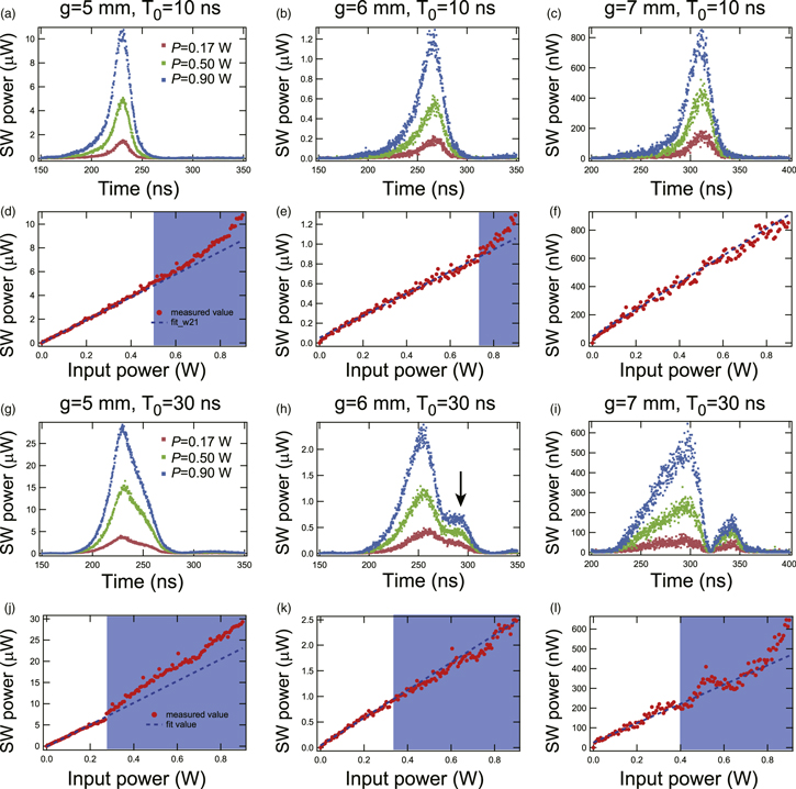
Fig. 3. (Color online) Time-domain SW signals in nonlinear regimes, converted into the power ( ) in propagating distances of (a) g = 5 mm, (b) g = 6 mm, and (c) g = 7 mm. The external magnetic field was set to be 1410 Oe. The duration of input pulse was fixed to be 10 ns. Corresponding input power dependences of SW (output) power in (d) g = 5 mm, (e) g = 6 mm, and (f) g = 7 mm were exhibited by solid circles. The broken line was inserted as an eye guide to see a linear relation between input and output powers. SW signals in nonlinear regime in case of input pulse duration 30 ns. The propagating distances were (a) g = 5 mm, (b) g = 6 mm, and (c) g = 7 mm. The input power dependences in each distance (j) g = 5 mm, (k) g = 6 mm, and (l) g = 7 mm were also shown by solid circles.
Download figure:
Standard image High-resolution imageIn each propagation distance g with fixed the excitation duration T0 = 10 ns, the SW signals become strong as increasing the input excitation power from 0.17 to 0.90 W. When the input excitation power reached to 0.90 W, we can easily recognize the larger SW in Figs. 3(a)–3(c). To investigate the nonlinear effect, the SW power dependence on input power was shown in Figs. 3(d)–3(f). In case of g = 5 mm, the SW power dependence deviates from a linear relation shown by the broken line at 0.49 W. In case of g = 6 mm, it deviates at 0.73 W. The SWs were actually in a nonlinear regime, showing the formation of SW soliton. In case of g = 7 mm, the power dependence fluctuates at higher Pin, however, we could not recognize the clear deviation even at Pin = 0.90 W. This means that the relaxation and dispersion effects prevent the formation of soliton, since the long propagation distance means an enough time to lose the nonlinear power. The nonlinear effect competes with the SW relaxation and dispersion.
To discuss this point, we evaluated the full-width at half-maximum (FWHM) ΔT for Figs. 3(a)–3(b) and shown in the Table I. At Pin = 0.17 W, the ΔT simply increases and represents the fact that the dispersion is always stronger than the nonlinear effect. The SW stays in the linear regime. While at Pin = 0.50 W, the soliton is only possible at g = 5 mm. After further propagation, at g = 6 mm, the dispersion becomes stronger than the nonlinear effect and the ΔT starts to increase. At Pin = 0.90 W, the soliton formation is possible at g = 5 mm and 6 mm. At g = 7 mm, the dispersion may stronger or same as the nonlinear effect.
Table I. The FWHM of the SW packets shown in Figs. 3(a), 3(a), and 3(c).
| Pin |
 (ns) (ns) |
 (ns) (ns) |
 (ns) (ns) |
|---|---|---|---|
| 0.17 W | 11.6 | 13.6 | 15.4 |
| 0.50 W | 11.2 | 15.4 | 16.0 |
| 0.90 W | 12.2 | 16.0 | 17.0 |
Similarly, if the excitation duration was increased to be T0 = 30 ns, we can recognize strong increase of SW power in each propagation distance g. As shown in Figs. 3(g) and 3(j) with g = 5 mm, the deviating threshold decreases to be 0.28 W and the magnitude of deviation from linear relation increases. In case of g = 6 mm, it is possible to see the second solitary-wave formation as shown by the arrow in Fig. 3(h). The second soliton was not separated from the first soliton. In Fig. 3(k), we plotted the power of the first soliton, and the SW power dependence appears to be linear relation. Here, the power contribution of second soliton was not considered. However, the relation starts to fluctuate at 0.32 W, representing 2-soliton formation. The input power is consuming to generate 2nd soliton.
In case of g = 7 mm, the 2-soliton formation becomes clear as shown in Fig. 3(i), which exhibits 2 independent SW solitons. The fluctuation in power dependence in Fig. 3(l) becomes larger at 0.4 W. The result represents that the longer duration T0 of excitation brings about stronger nonlinear effect than short excitation signal, since the total power Win = Pin × T0 is larger.
3.4. Evolution of SW soliton
As detected by the above experiments, the duration of excitation pulse plays a crucial role in the SW soliton formations. The time evolutions of SW solitons were depicted in Fig. 4.
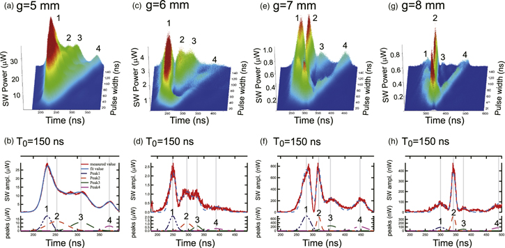
Fig. 4. (Color online) Evolution of SW solitons formation in propagating distances (a) g = 5 mm, (c) g = 6 mm, (e) g = 7 mm, and (g) g = 8 mm. The external magnetic field was set to be 1410 Oe. The input power was 0.60 W. The strong output amplitudes correspond to the SW solitons, labelled 1, 2, 3, and 4. To recognize the distance dependence, the cross section at the pulse duration 150 ns were depicted in case of (b) g = 5 mm, (d) g = 6 mm, (f) g = 7 mm, and (h) g = 8 mm. The broken line represents a multi-peaks analysis using the Gaussian functions.
Download figure:
Standard image High-resolution image
Figure 4(a) represents the formation of SW soliton in propagation distance g = 5 mm as a function of the excitation duration T0, with fixed input power Pin = 0.60 W. As clearly seen, the formation of SW soliton shows complicated process as increasing excitation duration. It is possible to detect the evolutions of 4-soliton propagation as labelled 1, 2, 3, and 4. However, each soliton is not perfectly separated from the others in time. To understand the 4-soliton propagation, the cross section of Fig. 4(a) at T0 = 150 ns is shown in the top panel of Fig. 4(b). By using a multi-peak analysis with Gaussian functions, we detected the position of each soliton shown in the bottom panel. The centers of each soliton are 231 ns, 253 ns, 308 ns, and 372 ns, respectively.
If the propagation distance is increased to be g = 6 mm [see Fig. 4(c)], we can see the separation of the 2nd and 3rd solitons from the others; 1st soliton at 250 ns and 4th at 390 ns soliton shows independent wave packet. From Fig. 4(d), only the 2nd and 3rd soliton shows an overlap. Increasing the propagation distance to be 7 mm, each soliton becomes independent showing the center positions at 280 ns, 319 ns, 355 ns, and 447 ns, respectively. Interestingly in case of g = 8 mm, the 1st and 3rd soliton are diminished but 2nd and 4th soliton keep their clear packet shapes.
To discuss the nonlinear effect, we analyzed the FWHM of solitons shown in Figs. 4(b), 4(d), 4(f), and 4(h). The magnitudes of FWHM are summarized in Table II.
Table II. The FWHM of the SW packets shown in Figs. 4(b), 4(d), 4(f), and 4(h).
| Pin |
 (ns) (ns) |
 (ns) (ns) |
 (ns) (ns) |
 (ns) (ns) |
|---|---|---|---|---|
| 1st | 23.4 | 24.3 | 29.9 | 33.3 |
| 2nd | 54.2 | 23.0 | 14.7 | 15.0 |
| 3rd | 52.6 | 38.5 | 38.9 | 33.0 |
| 4th | 27.5 | 50.1 | 49.9 | 42.6 |
We consider the 1st SW soliton. Since the Pin = 0.60 W is enough larger to cause nonlinear effect, we can consider the soliton propagation at g = 5 mm and g = 6 mm. However, at g = 7 mm, the FWHM (ΔT) slightly increases by 5.6 ns and starts to show the dispersion. For the 2nd soliton, it is possible to detect the clear decrease of ΔT at g = 6 mm. This corresponds to the separation from the other solitons. The FWHM (ΔT) keeps almost the same magnitude up to g = 8 mm. The dispersion and the nonlinear effect counterbalance with each other. In case of 3rd soliton, the decrease of ΔT is also observed at g = 6 mm. The ΔT is larger than 2nd soliton, however, it keeps the ΔT up to g = 8 mm. The 4th soliton shows a small ΔT only at g = 5 mm. At g = 6 mm, it increases to 50 ns. However, the ΔT keeps the same magnitude.
From the above analysis, there is the possibility that the nonlinear effects for 1st and 3rd solitons were consumed for the fusion and separation of wave packets (modulation instability). The 1st and 3rd solitons lose the nonlinear effects due to the overlap of waveforms and were diminished their amplitudes. While the 2nd soliton may absorb the nonlinear effects of 1st and 3rd solitons. Concerning to the 4th soliton, it exhibits a solitary shape already in g = 5 mm. The 4th soliton may not lose the nonlinear effect and could keep its shape up to g = 8 mm. This is the possible explanation why the 1st and 3rd solitons are diminished but 2nd and 4th soliton keep their clear packet shapes.
The competition between nonlinear effect and dispersion/relaxation shows a complicate behavior. As deeply discussed in the previous paper31), if we use the NLSE, it could be possible to deduce the characteristic time scales of dispersion, relaxation, and nonlinear effects. According to the Chen's analysis, we analyzed the simplest case of Fig. 4(a). The important time scales to consider are a relaxation time Tr, a dispersion time Td, a nonlinear response time Tn, and propagation time Tp given by

where η = 2.22 × 10⁶ rad s−1 is the characteristic decay time defined by  m s−1 is the group velocity,
  m2/rad s, N = −7.43 × 10⁹ rad s−1 is the nonlinear parameter,
  is the input power amplitude, in our experimental systems. The deduced values are listed in the Table III.
Table III. The parameters of nonlinear SW propagation for the case of Fig. 4(a).
| Time scale parameter | Tr (ns) | Td (ns) | Tn (ns) | Tp (ns) |
|---|---|---|---|---|
| 1-soliton | 450 | 954 | 190 | 195 |
From the Table III, we can understand that the nonlinear response time is smaller than the propagation time Tn < Tp, which means the nonlinear effect was effectively contribute to the soliton formation within the propagation. Furthermore, the relaxation time Tr and dispersion time Td is enough larger than Tn and Tp. This fact guarantees that the balance between nonlinear effect and dispersion effect to form soliton shape is possible during the propagation time.
To consider multi-soliton formation with the NLSE analysis, we should analyze data with a careful calculation, since we need to consider additional parameter of duration time T0. The detail comparison between 5 parameters for each independent soliton is beyond the scope of present paper. M. Chen et al. predicted 4-soliton propagation by using the NLSE, however, their experiments showed 3-soliton propagation. Although our experiment detected the 4-soliton propagation, we must be careful to compare with their NLSE analysis since material parameters are different from our system. The detail is left to be elucidated at this state, however, we clearly detected that the enough excitation power characterized by T0 = 150 ns is possible to cause 4 independent soliton propagation.
4. Conclusion
The nonlinear effect on SW was experimentally investigated by using fast RF switch and continuous wave generator method. We observed clear propagations in magnetostatic surface wave and backward volume wave modes in YIG waveguide. By choosing the backward volume waves which agree to the Lighthill criteria, we observed the nonlinear dependence on the input excitation power. The full-width at half-maximum of SW packets proved that the SW packet keeps its width and results in the soliton. By changing the excitation duration from 5 to 150 ns, the time evolution of SW soliton was investigated. The 4-soliton propagation was clearly detected in our experiments. The nonlinear effect to cause soliton generation competed with the relaxation/dispersion effect.
From an application viewpoint, the SW soliton propagation is the key issue for magnonic information technology. Though the control method of nonlinear effect is not obtained, the SW soliton showed that it is possible to keep a sharp packet in millimeter scale which is favorable for a signal transmission in magnonic chips. The understanding of nonlinear effect will be important in next development of magnonics.
Acknowledgments
This work is supported by the Grants-in-Aid for Scientific Research (19H00861 and 18H05346) from the Japan Society for the Promotion of Science (JSPS).