

Abstract
The 3D computer simulation based on the finite element method was performed to obtain the impedance in the presence/absence of adherent living cells. The sensitivity of the inter-digitated electrode was investigated by varying the width (W) and spacing (S) for different number of electrode fingers N. It was found that the peak sensitivity corresponding to W/S < 1 and W/S > 1 exhibited higher sensitivity than W/S = 1. However, the sensitivity was relatively large when W/S < 1. Furthermore, the slope of the peak sensitivity curve decreased with the increase in N, emphasizing the fact that it has greater impact on sensitivity than W/S. It is important to note that the peak sensitivity due to smaller electrode width results in higher sensitivity. Hence, the experimentalists are recommended to choose the smaller electrode geometry with smaller electrode width in order to realize better sensitivity in the presence of adherent cell.
Export citation and abstract BibTeX RIS
1. Introduction
Impedance measurements for monitoring living cells is widely accepted for its label free, non-invasive and quantitative assessment of cell status.1) The non-invasive aspect makes it effective for clinical point-of-care diagnostic applications with the leverage of simple, flexible and cost effective fabrication techniques.2,3)
The impedance measurements are preferred for biological cell monitoring as they automatically provide sensitive and accurate results. The various impedance sensing methods such as electrochemical impedance spectroscopy,4,5) impedance flow cytometry,6,7) and electric cell-substrate impedance sensing (ECIS)8) have been outlined.1) Among these the ECIS is a non-invasive and powerful tool to monitor cellular properties at a single cell resolution with high sensitivity and accuracy.9,10)
There are numerous electrochemical biosensors available for sensing by virtue of their optimization capacity, low cost and point-of-care testing.11) They consist of potentiometric sensors, amperometric sensors, and impedimetric/conductometric sensors.12) Among these, the impedimetric sensors are specifically preferred as they can operate at very low AC voltage,13) ease of miniaturization,11) and less prone to interference.14) Interdigitated electrodes (IDEs) and metal electrodes are the examples for impedimetric sensors. The IDEs are suitable for monitoring adherent cells,15,16) while the parallel facing electrodes are preferred for floating cell detection.17,18) This is due to the fact that the IDE has high electric field and current density concentration at the electrode vicinity owing to high sensitivity.19) There are several experimental works on IDE with living cells20–22) and without living cells.23,24) On the other hand, none of the simulation works on IDE geometry optimization included the existence of living cells.25–27) In addition to this, there are quite a few reports that address the factors influencing the sensitivity of IDE in the absence of living cells.28–31) Meanwhile, these issues were addressed in our previous report32) where the sensitivity due to IDE geometry was studied in the presence of adherent cell through 3D computer simulations. However, the sensitivity study was limited to the electrode geometry where the width (W) of the electrode was equal to the spacing (S) in the presence of adherent cell.
In this work the sensitivity study of IDE is extended for various W/S in the presence of adherent cell through 3D computer simulations. The electrode geometry is varied by varying the ratio of W and S in the presence of adherent cell in order to examine the best electrode geometry for achieving high sensitivity. We observed that the sensitivity increased with the increase in the number of electrode fingers (N) validating the results from our previous report.32) It was also found that the peak sensitivity corresponding to W/S < 1 and W/S > 1 exhibited higher sensitivity than W/S = 1. Moreover, the slope in the range of W/S < 1 showed the larger increase in sensitivity. Therefore, choosing the electrode geometry that is comparable to the cell size along with the smaller electrode width may benefit the experimentalists working on IDE in order to realize the maximum sensitivity in the presence of adherent cell.
This paper consists of the following sections: in Sect. 2 the simulation methods are explained. Section 3 illustrate the result and discussions, followed by the conclusion in Sect. 4.
2. Simulation methods
2.1. Simulation model
The conventional IDE sensor consists of two electrodes, working electrode (WE) and counter electrode (CE) where a large number of electrode fingers are arranged together to form a comb-like structure as shown in Fig. 1(a). A sinusoidal voltage is applied on the WE while the CE is grounded. Figure 1(b) shows the simulation model representing the unit domain of repetition in Fig. 1(a). The model illustrates the case where N = 4 and W = S = 15 μm. The parameters used for modeling are retained from our previous report,32) so that the transition from the previous work to the present work can be easily associated without any ambiguity. The unit domain has a fixed length of 120 μm, height of 240 μm, depth of 30 μm and only one cell is present in the simulation domain. The cell density on the actual IDE is therefore 250 cells mm−12,32) and it remains unchanged for the given domain area. The model is simulated for the three cases when N = 2, 4 and 6. Then, the W and S can be calculated by 120 μm/2N when W = S. The periodic boundary condition is applied on the adjacent faces of the y–z plane of the simulation model, while the mirror boundary condition is imposed on the faces on the x–z plane. This in fact demonstrates the efficient simulation of the actual IDE repetition due to structural symmetry. The electrode material used will not have significant influence on the impedance, and hence ignored in this work.

Fig. 1. (Color online) (a) Top view of inter-digitated electrode (IDE) (b) simulation model (N = 4, W = S = 15 μm) (c) adherent cell model.
Download figure:
Standard image High-resolution imageThe living cell is modeled as a hemisphere representing an adherent cell as shown in Fig. 1(c). The cell diameter is 10 μm.33) The gap between the cell and the electrode surface is 100 nm.34) The effect due to nucleus is not examined here as it has less influence on the ECIS signal.
The differential form of Maxwell's equations are solved using the finite element method using the COMSOL Multiphysics® 5.3a with AC/DC module.35) The parameter values were chosen based on our previous work as given in Table I.32) The frequency was swept between  and the user controlled meshing was implemented.
Table I. Parameters used in the simulation.
| Parameter | Value |
|---|---|
| Solution relative permittivity | 78 |
| Solution conductivity [S m−1] | 1.5 |
| Cell membrane relative permittivity | 6.0 |
| Cell membrane thickness [nm] | 5.0 |
| Cytoplasm relative permittivity | 60 |
| Cytoplasm conductivity [S m−1] | 0.5 |
| Double layer capacitance per unit area [Fm−2] | 0.89 |
2.2. Cell position average
In actual experimental setup, the living cells are distributed over random positions on the IDE surface. However, this situation is difficult to simulate due to high computational burden. For this reason, we have given a simplified model to take into account of the geometrical periodicity in IDE. We know that the probability of the existence of cells is uniform in space. Thus, it is relevant to take an average over all the possible cell positions within the domain in Fig. 1(b). Here, it will be sufficient to take the cell position average from the center of W to the center of S due to structural symmetry.32) As impedance value is unchanged by the cell position in y direction, we only consider possible cell positions in x direction. Considering that each situation could occur in parallel in the actual IDE sensor surface, we simulate impedance values for each possible cell positions in x and take a total impedance as parallel connections of those, as shown in Fig. 2. Then, the total impedance can be expressed as the weighted linear combination of admittances as follows:
where i represents possible cell positions in x between the center of W and center of S,  is the
  simulated impedance value, and
  is the
  weight originating from symmetry.32) The cells located at position 1 (center of W) and M (center of S) have the weight equal to 1. Likewise, the weight of the cells located from positions 2 to M − 1 are doubled. We set M = 9 as an optimum value to account for the precision and computation time. The simulation results in the next section will indicate such averaged impedance,

Fig. 2. Parallel impedance circuit representing the impedance for M cell positions.
Download figure:
Standard image High-resolution image3. Results and discussion
The sensitivity is defined as the increase rate of impedance magnitude in the presence of cell, which is given as

where  is the averaged impedance magnitude with cell and
  is that without cell.32)
3.1. Sensitivity due to varying electrode geometry
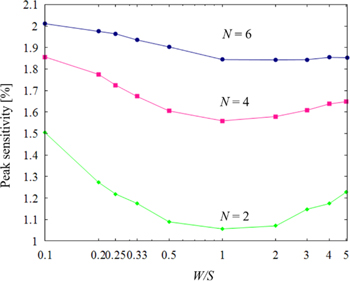
Figures 3(a)–3(c) shows the sensitivity plot where W and S are varied for N = 2, 4 and 6 respectively. The sensitivity is plotted as a function of frequency for three different W/S ratios. We may notice that the sensitivity curves show similar characteristics for the different cases of N. The reason for this is given in detail in our previous report32) by considering the sensitivity behavior at different frequency regions. The increase in sensitivity is observed for smaller W/S ratio for different electrode geometries. Figure 3(d) shows the peak sensitivity obtained from the sensitivity plot for different W/S ratios corresponding to N = 6. Later, the peak sensitivity values are extracted in a similar manner for each case of W/S corresponding to different values of N given in Table II. Thereafter, the peak sensitivity is plotted for all cases of N as a function of W/S. Figure 4 shows the peak sensitivity plot for different W/S ratios. The horizontal axis shows the W/S ratio corresponding to different N values. The vertical axis shows the peak sensitivity obtained from the sensitivity plot for different N in Fig. 3.

Fig. 3. (Color online) Sensitivity due to varying electrode geometry (a) N = 2 (b) N = 4 (c) N = 6. (d) Peak sensitivity extraction (N = 6).
Download figure:
Standard image High-resolution imageTable II. W/S ratio corresponding to different N values.
| N = 2 | N = 4 | N = 6 | ||||
|---|---|---|---|---|---|---|
| W/S | W(μm) | S(μm) | W(μm) | S(μm) | W(μm) | S(μm) |
| 0.1 | 5.5 | 54.5 | 3 | 27 | 2 | 18 |
| 0.2 | 10 | 50 | 5 | 25 | 3.3 | 16.7 |
| 0.25 | 12 | 48 | 6 | 24 | 4 | 16 |
| 0.33 | 15 | 45 | 7.5 | 22.5 | 5 | 15 |
| 0.5 | 20 | 40 | 10 | 20 | 6.6 | 13.4 |
| 1 | 30 | 30 | 15 | 15 | 10 | 10 |
| 2 | 40 | 20 | 20 | 10 | 13.4 | 6.6 |
| 3 | 45 | 15 | 22.5 | 7.5 | 15 | 5 |
| 4 | 12 | 48 | 24 | 6 | 16 | 4 |
| 5 | 50 | 10 | 25 | 5 | 16.7 | 3.3 |

Fig. 4. (Color online) Peak sensitivity plot for different N by varying W/S.
Download figure:
Standard image High-resolution imageAt first, we notice that the sensitivity increases with the increase in the number of electrode fingers N. In other words, the sensitivity increases for smaller electrode geometry. It is evident that the number of electrode edges increases with the increase in N. This implies that the current density or the electric field is concentrated along the electrode edges as shown in Fig. 5 as a result of which the sensitivity increases with the presence of cell on the electrode edges.28)

Fig. 5. (Color online) The vector distribution of current on the electrode edges when W/S = 1 for N = 2 at 106 Hz.
Download figure:
Standard image High-resolution imageSecond, the results in Fig. 4 shows that the peak sensitivity increases when W/S > 1 and W/S < 1. Figure 6 shows the current streamline and surface plots along with the schematic of adherent cell for the cases when W/S ≫ 1, W/S = 1 and W/S ≪ 1 respectively. When W/S > 1, W increases and S decreases due to which the cell is always present on the electrode. In this case, the denser electric field along S and the cell coverage on the electrode edges as shown in Fig. 6(a) result in the gentle increase in peak sensitivity when W/S > 1. However, the sensitivity increase in the range of W/S < 1 is significant as seen in Figs. 3(a)–3(c) and 4. This is due to the complete coverage of the cell on the electrode as well as the electrode edges as shown in Fig. 6(c) as a result of which the impedance due to current density is higher than W/S > 1. This results in increased sensitivity. For W/S = 1, the cell can be present only on one of the electrode edges irrespective of the cell position as seen in Fig. 6(b). This is true when the cell size is comparable or smaller than the electrode size. For this reason, the sensitivity due to W/S = 1 is smaller than W/S > 1 or W/S < 1.

Fig. 6. (Color online) Cross-sectional view of the current density surface and streamline plot along with the schematic of the adherent cell for N = 4 at 105 Hz (a) W/S ≫ 1 (b) W/S = 1 (c) W/S ≪ 1. The surface plot solves for log ∣J∣.
Download figure:
Standard image High-resolution imageNext, we see that the slope of the peak sensitivity curve in Fig. 4 decreases with the increase in N. As the electrode geometry becomes smaller, the changes due to W/S becomes negligible. This is due to the fact that the effect from the existence of the cell on the electrode edges becomes marginal once the cell has complete occupancy on the two electrode edges as shown in Fig. 6(c). Thereafter, the changes in impedance with respect to the further decrease in the electrode width in the presence of cell has less impact on sensitivity. For the case when N is small, the W and S are large in comparison to the cell size. Then the changes due to W/S has a greater influence as the cell coverage increases with the decrease in W and S. This in turn results in increased slope for smaller N as seen in Fig. 4.
We may also observe that the difference due to W/S is small compared to that due to N, as the number of the electrode edges for the given N remains unaltered considering the fact that the electrode edge has significant impact on sensitivity in comparison to the electrode ratio.
4. Conclusion
The sensitivity of IDE was examined in the presence of adherent cell for different W/S ratios by varying the electrode geometry. It was observed that the peak sensitivity increased with the increase in N due to increase in the number of electrode edges which in turn results in increased sensitivity. Also, it was found that the sensitivity was higher when W/S < 1 than when W/S > 1. The slope decreases for the smaller electrode geometry (N = 6) as the changes due to W/S is very small with the increase in N. This also indicates that the effect due to N is more significant than the electrode ratio. Therefore, we recommend that using smaller electrode geometry comparable to the cell size may be beneficial in order to obtain higher sensitivity in the presence of adherent cell. We also suggest that the smaller electrode width may be suitable for the experimentalists working with finer electrode geometry in order to obtain maximized sensitivity in the presence of adherent cell.
Appendix
There is no one strict method to find the cell position average. In our previous work32) the electrode ratio was fixed (W/S = 1). Hence, the changes due to impedance was not significant due to different cell positions. Therefore, the total impedance average was calculated by merely adding the impedance values in corresponding to M cell positions and then dividing with their corresponding weights given as follows:
where  is the
  weight and
  is the
  impedance, and M was taken as 9 in our work.
In this work, since we are considering varying electrode geometry, there can be a strong impact on impedance values obtained from different cell positions. Thus, it may be meaningful to consider a relatively strict averaging method based on the parallel impedance model for different cell positions as a result of varying W and S as explained in Sect. 2. However, we notice that the results obtained from both these methods as shown in Figs. 4 and A·1 are similar as the absolute impedance does not show any significant difference. Since, both the methods show similar behavior in the peak sensitivity plots, either methods can be adapted in taking the average due to cell positions.
Fig. A·1. (Color online) Peak sensitivity plot corresponding to series impedance average.
Download figure:
Standard image High-resolution image