The Limited Role of the Streaming Instability during Moon and Exomoon Formation

The origin of the Earth's Moon is a long-standing open problem in planetary science. While it is accepted that the Moon formed from a partially vaporized disk generated by a collision between the proto-Earth and an impactor approximately 4.5 billion yr ago (the "giant impact hypothesis"; Hartmann & Davis 1975; Cameron & Ward 1976), the details, such as the impactor radius and velocity, are actively debated. According to the canonical model, the proto-Earth was hit by a Mars-sized impactor (Canup & Asphaug 2001). This model can successfully explain several observations, such as the mass of the Moon, the angular momentum of the Earth–Moon system, and the small lunar core. Moreover, this model could potentially explain the observation that the Moon is depleted in volatiles, if they escaped during the impact or subsequent processes (see reviews by Halliday 2004; Canup et al. 2023). However, this model fails to explain the Earth and Moon's nearly identical isotopic ratios (e.g., Si, Ti, W, and O; Armytage et al. 2012; Zhang & Dauphas 2012; Touboul et al. 2015; Thiemens et al. 2019, 2021; Kruijer et al. 2021). This is because the disk generated by an oblique Mars-sized impactor is primarily made of the impactor materials (Canup 2004; Kegerreis et al. 2022; Hull et al. 2024), which likely had different isotopic ratios from Earth, unless the inner solar system was well mixed and homogenized (Dauphas 2017) or equilibrated in the disk phase (Pahlevan & Stevenson 2007; Lock et al. 2018). In contrast, more energetic impact models may solve this problem by mixing the proto-Earth and impactor. These energetic models include an impact between two half-Earth-sized objects (Canup 2012), an impact between a rapidly rotating proto-Earth and a small impactor (Cúk & Stewart 2012), and general impact events that involve high energy and high angular momentum, which create a doughnut-shaped vapor disk connected to the Earth (a so-called synestia; Lock et al. 2018). In these scenarios, the disk and the proto-Earth compositions could have been mixed well, potentially solving the isotopic problem. Other proposed scenarios include (a) the Moon formation by multiple small impacts (Rufu et al. 2017), (b) hit-and-run collisions that mix the proto-Earth and the Moon more than the canonical model does (Asphaug et al. 2021), and (c) an impact between the proto-Earth covered by a surface magma ocean and an impactor, which leads to more contribution from Earth to the disk than the canonical scenario (Hosono et al. 2019).

All of these models have potential explanations for the isotopic similarity, but each model faces challenges to explain other constraints. For example, the half-Earth and synestia models predict a much higher angular momentum of the Earth–Moon system than that of today (Canup 2012; Cúk & Stewart 2012). The excess of the angular momentum may or may not be removed easily (Cúk & Stewart 2012; Cúk et al. 2016, 2021; Rufu et al. 2017; Rufu & Canup 2020; Ward et al. 2020). Another constraint may come from the Earth's interior; the deep portion of the Earth still retains solar neon (Yokochi & Marty 2004; Williams & Mukhopadhyay 2019) and helium isotopic ratios (Williams et al. 2019), which are distinct from the rest of the mantle. These noble gases may have been delivered to Earth's mantle during the planet formation phase. This suggests that Earth's mantle developed chemical heterogeneity during Earth's accretion, when the protoplanetary disk was still present, and that the Earth's mantle has never been completely mixed, even by the Moon-forming impact. Previous work suggests that the preservation of the mantle heterogeneity can be explained by the canonical model but not by the energetic models, because these energetic impacts tend to mix the mantle (Nakajima & Stevenson 2015). It should be noted, however, the possibility that the neon and helium were delivered to the Earth's core and have been slowly leaking into the mantle over time has been discussed (Bouhifd et al. 2020), which would eliminate the need to preserve the mantle heterogeneity. However, it is not clear if delivery of these noble gases to the core was efficient.

Moreover, due to recent analytical capability, small isotopic differences between Earth and the Moon have been observed (e.g., K, O, W, V, Cr, and others; Wiechert et al. 2001; Kruijer et al. 2015; Touboul et al. 2015; Wang & Jacobsen 2016; Young et al. 2016; Thiemens et al. 2019; Nielsen et al. 2021; Sossi et al. 2018). Some isotopic difference, such as the Moon's enrichment in heavy K isotopes compared to those of Earth, can be explained by isotopic fractionation due to liquid–vapor phase separation during the Moon accretion process (Wang & Jacobsen 2016; Nie & Dauphas 2019; Charnoz et al. 2021). Observed small oxygen isotopic differences between Earth and the Moon may suggest that the Moon still records the impactor component (Cano et al. 2020). This suggestion may not be compatible with the energetic impact models because these impacts are so energetic that Earth and the Moon would be efficiently mixed. Whether the proposed models for the lunar origin can explain the observation that the Moon is depleted in volatiles is actively debated (Canup et al. 2015, 2023; Dauphas et al. 2015, 2022; Nakajima & Stevenson 2018; Sossi et al. 2018; Nie & Dauphas 2019; Charnoz et al. 2021; Halliday & Canup 2022; Canup et al. 2023).

Another key constraint that has not been discussed until recently is the vapor mass fraction (VMF) of the disk, which sensitively depends on the impact model. Less energetic impacts, such as the canonical model and the multiple impact model, produce relatively small VMFs (VMF ∼ 0.2 for the canonical model, Nakajima & Stevenson 2014, and ∼0.1–0.5 for the multiple impact model, Rufu et al. 2017), while more energetic models, such as the half-Earth model and synestia model, produce nearly pure vapor disks (VMF ∼0.8–1, Nakajima & Stevenson 2014). The VMF of the Moon-forming disk can significantly impact the Moon accretion process; if the initial Moon-forming disk is vapor-poor (liquid-rich), moonlets can quickly form by gravitational instability (GI) from the liquid layer in the disk midplane outside the Roche radius (Thompson & Stevenson 1988; Salmon & Canup 2012). These moonlets eventually accrete to the Moon in tens to hundreds of years (Thompson & Stevenson 1988; Salmon & Canup 2012; Lock et al. 2018). In contrast, an initially vapor-rich disk needs to cool until liquid droplets emerge before moonlet accretion begins. Growing moonlets in the vapor-rich disk experience strong gas drag from the vapor (Nakajima et al. 2022). The gas drag effect is strongest when the gas and moonlet are coupled to an adequate degree and is sensitive to the moonlet radius. It is strongest with a moonlet radius R_p of a few kilometers (Nakajima et al. 2022). In contrast, much smaller moonlets are completely coupled with the gas, and much larger moonlets are completely decoupled from the gas, experiencing a weaker gas drag effect. As a result, ∼kilometer-sized moonlets lose their angular momentum and inspiral onto the Earth within 1 day (Nakajima et al. 2022), a much shorter timescale than that required for lunar formation.

This same problem was a major challenge to planet formation in the protoplanetary disk (Adachi et al. 1976; Weidenschilling 1977). Here, we quickly review the gas drag problem in the protoplanetary disk. The radial velocity of a particle in a disk is (see Equation (A6) for the derivation; see also Armitage 2010; Takeuchi & Lin 2002)

$$\begin{eqnarray}&&{v}_{r}=\displaystyle \frac{{\tau }_{{\rm{f}}}^{-1}{v}_{r,{\rm{g}}}-2\eta {v}_{{\rm{K}}}}{{\tau }_{{\rm{f}}}+{\tau }_{{\rm{f}}}^{-1}},\end{eqnarray} \tag{ 1 }$$

where τ_f = Ωt_f is the dimensionless stopping time (Armitage 2010), Ω is the Keplerian angular velocity, t_f is the friction time (see further descriptions below), v_r,g is the gas velocity, and η is the pressure gradient parameter, described as

$$\begin{eqnarray}&&\eta =-\displaystyle \frac{1}{2}{\left(\displaystyle \frac{{c}_{{\rm{s}}}}{{v}_{{\rm{K}}}}\right)}^{2}\displaystyle \frac{\partial \mathrm{ln}{p}_{{\rm{g}}}}{\partial \mathrm{ln}r},\end{eqnarray} \tag{ 2 }$$

where c_s is the sound speed, v_K is the Keplerian velocity, p_g is the gas pressure, and r is the radial distance. v_r is largest when τ_f = 1. The friction time is the time until the particle and gas reach the same velocity and is defined as t_f = mv_rel/F_D, where m is the particle mass, v_rel is the relative azimuthal velocity between the gas and particle, and F_D is the drag force. In the protoplanetary disk, the gas drag for a particle is generally written as ${F}_{{\rm{D}}}=-\tfrac{{C}_{{\rm{D}}}}{2}\pi {\rho }_{{\rm{g}},0}{R}_{{\rm{p}}}^{2}{v}_{\mathrm{rel}}^{2}$, where C_D is the gas drag coefficient, ρ_g,0 is the initial gas density at the midplane, and R_p is the particle radius. The gas drag coefficients are roughly (Armitage 2010)

$$\begin{eqnarray}{C}_{{\rm{D}}}=\left\{\begin{array}{cc}24{\mathrm{Re}}^{-1}, & \mathrm{Re}\,\lt \,1(\mathrm{Stokes}\mathrm{regime})\\ 24{\mathrm{Re}}^{-0.6}, & 1\lt \mathrm{Re}\,\lt \,800(\mathrm{transition}\mathrm{regime})\\ 0.44, & \mathrm{Re}\,\gt \,800(\mathrm{Newton}\mathrm{regime})\end{array}\right.,\end{eqnarray} \tag{ 3 }$$

where Re is the Reynolds number. Assuming that v_rel ∼ η v_K (see Equation (A2)), ν ∼ c_s λ, where ν is the kinematic viscosity, λ is the mean free path ($\lambda =\tfrac{{k}_{{\rm{B}}}T}{\sqrt{2}\pi {d}^{2}{p}_{{\rm{g}},0}}$, where k_B is the Boltzmann constant, T is the temperature, d is the molecular diameter, and p_g,0 is the gas pressure at the midplane), Re = $\tfrac{{v}_{\mathrm{rel}}{R}_{p}}{\nu }\sim 4.26$, which is in the transition regime, in the protoplanetary disk at 1 au, assuming T = 280 K, η = 0.002, d = 289 pm, R_p = 0.52 m (see discussion below), ${p}_{{\rm{g}},0}=\tfrac{{\rho }_{g,0}{RT}}{{m}_{{\rm{m}}}}$, and m_m = 0.002 kg mol^–1, where m_m is the mean molecular weight and R is the gas constant. Here we also assume the following vertical distribution of the gas density ρ_g,

$$\begin{eqnarray}&&{\rho }_{{\rm{g}}}={\rho }_{{\rm{g}},0}\exp \left(-\displaystyle \frac{{z}^{2}}{2{H}^{2}}\right),\end{eqnarray} \tag{ 4 }$$

where z is the vertical coordinate and H is the gas scale height. This leads to ${\rho }_{{\rm{g}},0}=\tfrac{{{\rm{\Sigma }}}_{{\rm{g}}}}{\sqrt{2\pi }H}$. We assume Σ_g = 17,000 kg m⁻² and use the relationships of ${c}_{s}=\sqrt{{RT}/{m}_{{\rm{m}}}}$, H = c_s /Ω, $\tfrac{\partial \mathrm{ln}{p}_{{\rm{g}}}}{\partial \mathrm{ln}r}\,=(-3+\beta /2)$, and $\beta =\tfrac{1}{2}$. The orbital angular frequency is ${\rm{\Omega }}=\sqrt{{GM}/{r}^{3}}$, where G is the gravitational constant, M is the stellar mass and r is the distance from the star (for the Moon-forming disk, M is the Earth mass and r is the distance from Earth). These parameters are taken from previous work (Carrera et al. 2015; other values of β have been discussed, such as $\beta =\tfrac{3}{7}$; Chiang & Youdin 2010).

The dimensionless stopping time becomes

$$\begin{eqnarray}&&{\tau }_{{\rm{f}}}={\rm{\Omega }}{t}_{{\rm{f}}}={\rm{\Omega }}\displaystyle \frac{8}{3{C}_{{\rm{D}}}}\displaystyle \frac{{\rho }_{{\rm{p}}}{R}_{{\rm{p}}}}{{\rho }_{{\rm{g}},0}{v}_{\mathrm{rel}}}=\displaystyle \frac{8}{3{C}_{{\rm{D}}}\eta }\displaystyle \frac{{\rho }_{{\rm{p}}}{R}_{{\rm{p}}}}{{\rho }_{{\rm{g}},0}r}.\end{eqnarray} \tag{ 5 }$$

τ_f = 1 when R_p = 0.52 m. The particle density ρ_p = 3000 kg m⁻³ is assumed. The residence time of the particle at 1 au is 1 au/v_r = 75 yr, where v_r is the radial fall velocity of the particle (see Equation (A7); for simplicity, the radial gas velocity v_r,g = 0 is assumed). Thus, an approximately meter-sized particle falls toward the Sun at 1 au within 80 yr, a timescale much shorter than the planet formation timescale (several tens of Myr). This is the so-called "meter barrier" problem, which was a major issue to explain planetary growth in a classical planet formation model (Adachi et al. 1976; Weidenschilling 1977).

In contrast, for the vapor-rich Moon-forming disk, τ_f = 1 ($\mathrm{Re}\,\gt \,{10}^{10}$) is achieved when R_p = 1.8 km, assuming ρ_g,0 = 40 kg m^–3, ρ_p = 3000 kg m^–3, r = 3 R_⊕, η = 0.04, T = 5200 K (see Section 2.3 for justifications for these parameters), and d = 300 pm. The residence time, r/v_r , is approximately 1 day (1.21 days), which is much shorter than the Moon-formation timescale of several tens of yr to 100 yr. This formation timescale is ultimately determined by the radiative cooling timescale, but it is model-dependent. Here we provide a very simple estimate; the timescale for radiative cooling is $\tfrac{{M}_{\mathrm{disk}}(L+{C}_{p}{\rm{\Delta }}T)}{4\pi {r}^{2}\sigma {T}_{\mathrm{ph}}^{4}}\sim 10$ yr (this is also consistent with numerical work; Lock et al. 2018), where M_disk is the disk mass, L is the latent heat, C_p is the specific heat, ΔT is the temperature change over time, σ is the Stefan–Boltzmann constant, and T_ph is the photosphere temperature. Here, M_disk ∼ 0.015 M_⊕, L = 1.2 × 10⁷ J kg^–1 (Melosh 2007), C_p = 10³ J K^–1 kg^–1, ΔT = 2000 K, and T_ph = 2000 K (Thompson & Stevenson 1988) are assumed. However, the actual Moon-formation timescale can be longer than this for several reasons, including additional heating due to viscous spreading (Thompson & Stevenson 1988; Charnoz & Michaut 2015) and radial material transport efficiency (e.g., Salmon & Canup 2012). A short Moon-formation timescale has been proposed (e.g., Mullen & Gammie 2020; Kegerreis et al. 2022), but the typical Moon-formation timescale has been estimated to range in 10–10² yr.

The vertical settling velocity of condensing particles is ${v}_{\mathrm{settle}}=\sqrt{\tfrac{8}{3{C}_{{\rm{D}}}}\tfrac{{\rho }_{{\rm{p}}}{R}_{{\rm{p}}}{{\rm{\Omega }}}^{2}z}{{\rho }_{{\rm{g}}}}}$ (Armitage 2010). Assuming z ∼ H, the settling time for a particle with a radius off 2 is 0.22 days. Determining the collision history of moonlets requires conducting orbital dynamics simulations, but here we provide a rough estimate. A rough estimate of the mass-doubling time of the largest moonlet in the Moon-forming disk is typically ∼1 day (Salmon & Canup 2012). If a 2 km-sized moonlet mass doubles in a day, the radius change is very small (2 km × 2^1/3 = 2.5 km), and the gas drag effect remains strong on such a moonlet; this change does not prevent the moonlet from falling into Earth. However, the actual collision time can vary depending on the local concentration of particles, which needs a detailed future study.

This gas drag effect is a problem with forming the Moon from an initially vapor-rich disk. The Moon can still form after most of the vapor condenses, but by that time a significant portion of the disk mass could be lost (Ida et al. 2020; Nakajima et al. 2022), which would fail to form a large moon from an initially vapor-rich disk (here we use a "large" moon when its mass is ∼1 wt% or larger of the host planet). If this is the case, an initially vapor-rich disk may not be capable of forming a large Moon (Nakajima et al. 2022). In contrast, the gas drag effect is weak for vapor-poor disks, which are generated by less energetic models, such as the canonical and multiple impact models.

A potential solution to this vapor drag problem is forming a large moonlet very quickly (much larger than 2 km), so that the moonlet would not experience strong gas drag. This is the accepted solution for the gas drag problem in the protoplanetary disk. The proposed mechanism is the streaming instability (Youdin & Goodman 2005; Johansen et al. 2007), where particles spontaneously concentrate in the disk, gravitationally collapsing and forming a large clump (∼100 km in size; Johansen et al. 2015). If this mechanism works for the Moon-forming disk, an initially vapor-rich disk may be able to form the Moon despite the gas drag issue. If this mechanism turns out not to work for the Moon-forming disk, it is an interesting finding as well, given that a Moon-forming disk is often treated as a miniature analog of the protoplanetary disk. Understanding what makes these two disks differ would deepen our understanding of planet and satellite formation processes.

Moreover, knowing whether the streaming instability can affect moon formation processes informs our understanding of moon formation in the solar and extrasolar systems. Moon formation in an impact-induced disk is common in the solar system (e.g., the moons of Mars (Craddock 2011), the moons of Uranus (Slattery et al. 1992), and Pluto-Charon (Canup 2005)). While there are no confirmed exomoons (moons around exoplanets) to date (e.g., Cassese & Kipping 2022), impact-induced exomoons should be common because impacts are a common process during planet formation (Nakajima et al. 2022) and because impacts in extrasolar systems may have already been observed (e.g., Meng et al. 2014; Bonomo et al. 2019; Thompson et al. 2019; Kenworthy et al. 2023). If streaming instability operates in these disks, it can affect what types of planets can host exomoons, which can be compared with future exomoon observations.

It should also be noted that other instability, such as secular GI (e.g., Youdin 2011; Takahashi & Inutsuka 2014; Tominaga et al. 2018) and two-component viscous GI (TVGI; Tominaga et al. 2019), have been discussed as a mechanism for planetesimal and dust ring formation. The secular GI occurs when dust–gas interaction reduces the rotational support of the rotating disk, which leads to dust concentration. The TVGI is an instability caused by dust–gas friction and turbulent gas viscosity. These instabilities can lead to clump formation even if the disk is self-gravitationally stable. The implications of these instabilities are beyond the scope of this paper.

The goal of this work is to investigate whether the streaming instability can form moonlets that are large enough to avoid strong gas drag from the vapor-rich disk. The result could constrain the Moon-formation model as well as general impact-induced models in the solar and extrasolar systems. We conduct hydrodynamic simulations using the code Athena (Stone et al. 2008; Bai & Stone 2010a). We first conduct 2D simulations to identify the section of parameter space that leads to streaming instability. Subsequently, we conduct 3D simulations with self-gravity to identify the size distribution of the moonlets. Finally, we identify the lifetime of the moonlets formed by streaming instability to investigate whether it is possible to form a large moon from an initially vapor-rich disk. For the general impact-induced disks, we consider "rocky" and "icy" disks, where these disks form by collisions between rocky planets (with silicate mantles and iron cores) and between icy planets (with water-ice mantles and silicate cores), respectively.

We use the Athena hydrodynamics code, which solves the equations of hydrodynamics using a second-order accurate Godunov flux-conservative approach (Stone et al. 2008). We use the configuration of Athena that couples the dimensionally unsplit corner transport upwind method (Colella 1990) to the third-order in-space piecewise parabolic method by Colella & Woodward (1984) and calculates the numerical fluxes using the HLLC Riemann solver (Toro 1999). We also integrate the equations of motion for particles following Bai & Stone (2010a) and include particle self-gravity for 3D simulations following the particle-mesh approach described in previous work (Simon et al. 2016). Orbital advection is taken into account following previous work (Bai & Stone 2010a, 2010b). Our setup is the local shearing box approximation in which a small patch of the disk is corotating with the disk at the Keplerian velocity (Stone & Gardiner 2010). The local Cartesian frame is defined as (x, z) for 2D and (x, y, z) for 3D simulations, with x as the radial coordinate from the planet, z parallel to the planetary spin axis, and y in the direction of the orbital rotation.

In the Athena code, we solve the following equations for our simulations (Bai & Stone 2010a; Simon et al. 2016; Li et al. 2019):

$$\begin{eqnarray}&&\displaystyle \frac{\partial {\rho }_{{\rm{g}}}}{\partial t}+{\rm{\nabla }}\cdot ({\rho }_{{\rm{g}}}{\bf{u}})=0,\end{eqnarray} \tag{ 6 }$$

$$\begin{eqnarray}&&\begin{array}{l}\displaystyle \frac{\partial {\rho }_{{\rm{g}}}{\bf{u}}}{\partial t}+{\rm{\nabla }}\cdot ({\rho }_{{\rm{g}}}{\bf{uu}}+{p}_{g}{\bf{I}})\\ =\,3{\rho }_{{\rm{g}}}{{\rm{\Omega }}}^{2}{\bf{x}}-{\rho }_{{\rm{g}}}{{\rm{\Omega }}}^{2}{\bf{z}}-2{\rho }_{{\rm{g}}}{\boldsymbol{\Omega }}\times {\bf{u}}+{\rho }_{{\rm{p}}}\displaystyle \frac{\overline{{\bf{v}}}-{\bf{u}}}{{t}_{{\rm{f}}}},\end{array}\end{eqnarray} \tag{ 7 }$$

$$\begin{eqnarray}&&\begin{array}{l}\displaystyle \frac{d{{\bf{v}}}_{i}}{{dt}}=-2\eta {v}_{{\rm{K}}}{\rm{\Omega }}\hat{{\bf{x}}}+3{{\rm{\Omega }}}^{2}{x}_{i}\hat{{\bf{x}}}\\ -{{\rm{\Omega }}}^{2}{z}_{i}\hat{{\bf{z}}}-2{\boldsymbol{\Omega }}\times {{\bf{v}}}_{i}-\displaystyle \frac{{{\bf{v}}}_{i}-\overline{{\bf{u}}}}{{t}_{{\rm{f}}}}+{{\bf{a}}}_{{\rm{g}}}.\end{array}\end{eqnarray} \tag{ 8 }$$

The first two equations specify mass and momentum conservation for the gas, respectively, while the third equation represents the motion of a particle i coupled with the gas. Here, u is the velocity of the gas and I is the identity matrix. $\overline{{\bf{v}}}$ is the mass-weighted averaged particle velocity in the fluid element, assuming that particles can be treated as fluid (Bai & Stone 2010a). The terms of the right-hand side of Equation (7) are radial tidal forces (gravity and centrifugal force), vertical gravity, and the Coriolis force and the feedback from the particle to the gas. In Equation (8), the first term on the right-hand side describes a constant radial force due to gas drag. v _i is the particle velocity, $\hat{{\bf{x}}}$ and $\hat{{\bf{z}}}$ represent the unit vectors in the x- and z-directions, and x_i and z_i are the values of x and z for the particle i. $\overline{{\bf{u}}}$ is the gas velocity interpolated from the grid cell centers to the location of the particle. The second, third, and fourth terms are radial and vertical tidal forces and the Coriolis force. a _g is the acceleration due to self-gravity, which is considered only in 3D simulations. a _g = −∇Φ_p , where Φ_p is the gravitational potential and satisfies the Poisson's equation, ∇²Φ_p = 4π G ρ_p . To reduce computational time, the particles are organized into "superparticles," each representing a cluster of individual particles of the same size. In the code units, we normalize Ω = c_s = H = ρ_g,0 = 1. The gas and particle initial distributions are described in Equation (4) and as

$$\begin{eqnarray}&&{\rho }_{{\rm{p}}}=\displaystyle \frac{{{\rm{\Sigma }}}_{{\rm{p}}}}{\sqrt{2\pi }{H}_{{\rm{p}}}}\exp \left(-\displaystyle \frac{{z}^{2}}{2{H}_{{\rm{p}}}^{2}}\right),\end{eqnarray} \tag{ 9 }$$

respectively, where H_p is the scale height of the particles and is set to 0.02H (Bai & Stone 2010a) and Σ_p is the particle surface density. The system uses an isothermal equation of state $P={\rho }_{g}{c}_{s}^{2}$, and the particles are distributed uniformly in the x- and y-directions and normally in the z-direction (Equation (9)). The computational domains are 0.2H × 0.2H in 2D simulations and 0.2H × 0.2H × 0.2H in 3D simulations, with all-periodic boundary conditions. The resolution for 2D is 512 × 512, and each grid cell has one particle (512 × 512 = 262,144 particles). The resolution for 3D is 10 × 128³ (= 21 million particles in total). Previous work shows that the resolution of 128³ can produce the large clump size distribution well compared to those with 256³ and 512³ (Simon et al. 2016); therefore, this resolution of our 3D simulations is sufficient to resolve large clumps, which are the focus of this work. The initial particle size is assumed to be constant. Variable initial particle sizes could affect the growth speed (Krapp et al. 2019) and the concentrations of particles depending on their sizes (Yang & Zhu 2021), but it is not known to affect the largest clump size formed by streaming instability.

After we conduct 2D simulations, we identify filaments forming in the disk in order to constrain the parameter space favorable for the streaming instability. We use the Kolmogorov–Smirnov (KS) method, which is based on previous work (Carrera et al. 2015). For each time step in a given time window (25/Ω in our case), we compute the particle surface density ${{\rm{\Sigma }}}_{p}(x)={\int }_{-0.1}^{0.1}{\rho }_{p}(x,z){dz}$ and average it over the time window to give ${\left\langle {{\rm{\Sigma }}}_{p}\right\rangle }_{t}$. We then sort the values in ${\left\langle {{\rm{\Sigma }}}_{p}\right\rangle }_{t}$ from highest to lowest and compute the cumulative distribution of this sorted data set. Finally, we use the KS test to output a p-value that measures the likelihood that the underlying cumulative distribution was linear:

$$\begin{eqnarray}&&\begin{array}{l}Q(z)=2\displaystyle \sum _{j=1}^{\infty }{\left(-1\right)}^{j-1}{e}^{-2{z}^{2}{j}^{2}}\\ p=Q(D\sqrt{n}),\end{array}\end{eqnarray} \tag{ 10 }$$

where D is the maximum distance between the data and linear cumulative distributions and n is the number of data points. The higher the p is, the more homogeneous the system is, and therefore filament formation is unlikely, whereas a small p indicates filament formation is more likely. Here we assume that filament formation is very likely when p < 0.10, the same as in previous work (Carrera et al. 2015).

For self-gravitating clump detection in our 3D simulations, we use PLanetesimal ANalyzer (PLAN; Li et al. 2019). This is a tool to identify self-gravitating clumps specifically made for Athena output. The density of each particle is assessed based on the nearest particles. Particles with densities higher than a threshold are associated with neighboring dense particles until a density peak is achieved. In contrast, particle groups with a saddle point less than a threshold remain separated. Detailed descriptions are found in previous work (Li et al. 2019).

The main parameters for the Athena simulations are (1) the dimensionless stopping time τ_f (the Newton regime; see Section 1.2 and Nakajima et al. 2022), (2) the normalized pressure parameter Δ = η v_K/c_s, (3) the ratio of the particle surface density to the gas surface density Z = Σ_p/Σ_g (VMF = $\tfrac{1}{1+Z}$), and (4) the normalized gravity $\tilde{G}\equiv 4\pi G{\rho }_{{\rm{g}},0}/{{\rm{\Omega }}}^{2}$ for 3D simulations, where G is the gravitational constant. A small value of τ_f indicates a small particle radius R_p, where the particle is well coupled with the gas, whereas a large value of τ_f corresponds to a large value of R_p, which is more decoupled from the gas. A large value of Δ corresponds to a large pressure gradient and quicker radial infall. $\tilde{G}$ represents the strength of the self-gravity. The parameter space we are exploring for our 2D simulations is τ_f = 10⁻³, 10⁻², 10⁻¹, 10⁰, 10¹; Δ = 0.1, 0.2, 0.3, 0.4, 0.5; and Z = 0.05 and 0.1. For 3D simulations, we use Z = 0.1 and 0.3 and $\tilde{G}=0.1788$ and 0.5898, where the former $\tilde{G}$ value corresponds to a slightly cooler temperature (4700 K), while the latter corresponds to a hotter temperature (5200 K). Here, we justify the choice of these parameters. This range of τ_f corresponds to the particle radii between 2 m and 20 km (see Equation (5)). The global disk structures have been calculated based on hydrodynamic simulations in previous work. The overall disk mass of the Moon-forming disk is typically a few percent of Earth, depending on the impact model (M_D /M_L = 1.35–2.80, where M_D is the disk mass and M_L is the lunar mass; Nakajima & Stevenson 2014). The midplane disk temperature ranges from 3000 K to 7000 K, and the radial range of the disk is ∼1–8 R_⊕ (see Figure 5 in Nakajima & Stevenson 2014). The disk temperature is ∼4000–5500 K at r = 3 R_⊕. For the general rocky and icy impact-induced disks, the disk temperature can vary, typically in the range of thousands of K for vapor-rich disks (Nakajima et al. 2022). The pressure gradient can vary, but the typical value of η is ∼0.02–0.06 based on impact simulations (Nakajima et al. 2022). In the Moon-forming disk, the value of Z increases as the disk cools (on a timescale of 10–10² yr). In other words, Z can initially be zero in an energetic Moon-forming impact model (e.g., Lock et al. 2018) and eventually becomes infinity as the disk materials condense and the gas disappears. Thus, picking a value of Z means that we are seeing physics at a specific time. Since we are primarily interested in high-vapor disks (i.e., an early phase of the disk), we explore the mass ratio range Z ∈ [0.05, 0.1] for our 2D simulations and Z ∈ [0.1, 0.3] for our 3D simulations. We use the large value of Z = 0.3 as a sensitivity test. Higher values of Z can be achieved as the disk cools, but we focus on small values of Z (≤0.3) for several reasons. First, at a larger value of Z (>0.3), the conventional GI in the liquid part of the disk can form moonlets. At Z $\tfrac{1}{Z+1}=0.76$, and the total (Σ_p + Σ_g) surface density at r ∼ 3 R_⊕ is ∼10⁸ kg m⁻² in energetic models, which means that Σ_p = 0.76 × 10⁸ kg m⁻² = 7.6 × 10⁷ kg m⁻². Previous work suggests that when the liquid (melt) layer's thickness reaches 5–10 km (or the equivalent surface density of a few 10⁷ kg m⁻²), GI can happen in the melt layer (Machida & Abe 2004). Whether streaming instability occurs at the same time or whether streaming instability affects the GI in the Moon-forming disk are unknown and have not been explored in previous studies. Under these circumstances, the important of streaming instability becomes unclear. Additionally, these streaming instability simulations have been conducted at low-Z values (≤0.1) in previous work to reproduce conditions in the protoplanetary disks (e.g., Abod et al. 2019; Li & Youdin 2021), and simulations with high-Z (>0.3) values have not been fully tested. For these reasons, we focus on relatively small values of Z in this study.

For the set of Athena simulations, we focus on reproducing two sets of the Moon-forming disk thermal profile; assuming M = M_⊕ and r = 3 R_⊕, where M_⊕ is the Earth mass and R_⊕ is the Earth radius, the gas pressure at the midplane around 3 R_⊕ is ≈12 MPa, T = 4700 K, and m_m = 30 g mol⁻¹. This makes the density ρ_g,0 = 12.13 kg m⁻³ for an ideal gas, c_s = 1140 m s⁻¹, v_K = 4562 m s⁻¹, Ω = 2.38 × 10⁻⁴ s⁻¹, the scale height H = c_s /Ω = 4.78 × 10⁶ m, and $\tilde{G}=0.1788$. For the higher-temperature scenario, T = 5200 K, ρ_g,0 = 40.01 kg m⁻³, c_s = 1200 m s⁻¹, H = 5.03 × 10⁶, and $\tilde{G}=0.5898$. These temperatures are motivated by previous hydrodynamic calculations of the Moon-forming disk formation (Nakajima & Stevenson 2014), and the other parameters are calculated based on an equation of state of dunite assuming that the vapor and liquid phases are in equilibrium (MANEOS; Thompson & Lauson 1972; Melosh 2007). Since we are assuming that the disk is in liquid–vapor equilibrium, a higher disk temperature leads to a higher vapor density at the midplane. For example, the gas density at liquid–vapor equilibrium is 150 kg m⁻³ at 6000 K and 1.8 kg m⁻³ at 4000 K for dunite, according to MANEOS (Thompson & Lauson 1972; Melosh 2007). Assuming η ∼ 0.02–0.06 for the Moon-forming disk, Δ ∼ 0.1–0.2. However, higher values are possible (Nakajima et al. 2022); therefore, we explore the range of Δ ∼ 0.1–0.5.

The parameter values of Δ and $\tilde{G}$ are significantly different from values in the protoplanetary disk, where the typical values used are Δ ∼ 10⁻³–10⁻² and $\tilde{G}\sim 0.05$ in the protoplanetary disk (Carrera et al. 2015; Simon et al. 2016). We use a fixed value of Z in hydrodynamic calculations because the condensation timescale (∼years) is longer than the simulation timescale (we run 2D simulations for ∼100 orbits, which correspond to 123 hr. A steady state is reached by this time). We also assume that the disk does not evolve on this short timescale.

Figure 1(A) shows four examples of spacetime plots of our 2D simulations, where (1) (τ_f, Δ) = 10⁻³, 0.3, (2) 10⁻², 0.1, (3) 10⁻¹, 0.2, and (4) 10⁻¹, 0.2. Z = 0.1 for the four cases. These simulations represent four characteristic regimes. The horizontal axis is x normalized by the scale height H, and the vertical axis is the number of orbits. The color shows particle concentration. In case 1, τ_f is small, which means that gas and particles are well coupled, and this does not lead to filament formation. In case 2, after ∼20 orbits, filaments start forming, and these filaments are stable during the rest of the simulations, which indicate that streaming instability occurs with this chosen parameter. A radially shearing periodic boundary condition is used in the x-direction; therefore, the filament that appears at x/H = −0.1 at ∼100 orbits reappears at x/H = 0.1. Two distinct filaments form in this simulation. In case 3, filaments form, but they are not stable because their radial movements are high due to the high Δ value. Thus, this is not an ideal parameter space for streaming instability. Similar behaviors have been seen in simulations for the protoplanetary disk with other parameter combinations (e.g., Δ = 0.05, τ_f = 3, Z = 0.005; Carrera et al. 2015). In case 4, the filaments are not as clearly defined as those in case 2, but a coherent filament structure is found after several orbits. Thus, this is also considered as a streaming instability regime.

Zoom In Zoom Out Reset image size

Figure 1(B) shows the summary of our 2D simulations for Z = 0.1 (top) and Z = 0.05 (bottom). We use the KS test to identify the extent of particle concentration (see Section 2.2). Concentration is measured by the p-value, and when the value of p is small (p < 0.1), streaming instability is likely (Carrera et al. 2015). The color bar indicates the p-value. For Z = 0.1, p < 0.1 is achieved when Δ = 0.1 and 10⁻³ ≤ τ_f ≤ 10⁰. For large Δ values, the radial motions are large, and stable filaments do not form, as discussed above. For Z = 0.05, this trend remains the same, but the streaming instability regime is smaller (10⁻² ≤ τ_f ≤ 10⁰) than that for Z = 0.1. This is because the larger Z leads to the presence of more particles in the disk and therefore to more filament formation (Carrera et al. 2015). Thus, our 2D simulations show that the most filaments form at relatively small Δ (Δ = 0.1) and with both Z = 0.1 and Z = 0.05, but the higher Z has more favorable conditions. This general trend is consistent with previous work in the protoplanetary disk (e.g., Carrera et al. 2015), which investigates smaller Δ values for the protoplanetary disk (Δ ≤ 0.05).

Now that we have identified the parameter space for the streaming instability (Δ = 0.1, Z = 0.1), we perform 3D simulations with self-gravity to estimate the size distributions of streaming-instability-induced moonlets. Figure 2 shows snapshots of one of our 3D simulations (${\tau }_{f}=1,\tilde{G}\,=0.5898,Z=0.1$, and Δ = 0.1) at four different times (t = 0.32, 2.87, 3.39, and 3.55), where t is the number of orbits. The self-gravity is not initially included and is turned on at t = 3.18. This is a general practice to avoid artificial clumping before streaming instability takes place (Simon et al. 2016). The color shows the particle density. The circles indicate the Hill spheres of self-bound clumps, which are identified using PLAN (Li et al. 2019). At t = 0.32, no clump is identified, but by t = 2.87, the streaming instability fully develops and reaches its steady state. After self-gravity is turned on at t = 3.18, self-gravitating clumps form right away (t = 3.39). This general behavior is similar to previous work on the streaming instability in the protoplanetary disk (Abod et al. 2019), but the time it takes to form clumps by streaming instability is shorter, probably because of the large Z value (Simon et al. 2022) compared to those of the protoplanetary disk.

Zoom In Zoom Out Reset image size

Figure 3(A) shows the cumulative distribution of moonlet mass M_p , normalized by the characteristic self-gravitating mass M_G , defined as (Abod et al. 2019)

$$\begin{eqnarray}&&\begin{array}{l}{M}_{G}=\pi {\left(\displaystyle \frac{{\lambda }_{G}}{2}\right)}^{2}{{\rm{\Sigma }}}_{p}=4{\pi }^{5}\displaystyle \frac{{G}^{2}{{\rm{\Sigma }}}_{p}^{3}}{{{\rm{\Omega }}}^{4}}\\ =\displaystyle \frac{\sqrt{2}}{2}{\pi }^{9/2}{Z}^{3}{\tilde{G}}^{2}({\rho }_{{\rm{g}},0}{H}^{3}),\end{array}\end{eqnarray} \tag{ 11 }$$

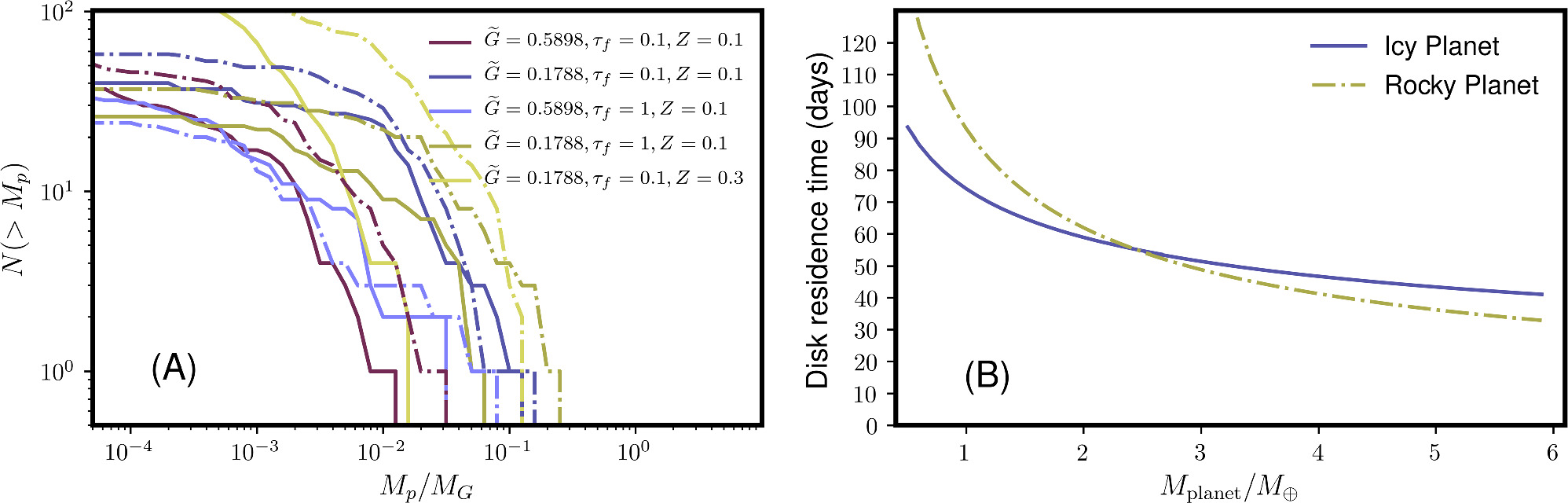
where λ_G is an instability wavelength, which originates from the Toomre dispersion relation, equating the tidal and gravitational forces (Abod et al. 2019). The parameters are τ_f = 0.1, 1, $\tilde{G}=0.1788,0.5898$, and Z = 0.1, 0.3. For the $\tilde{G}=0.1787$ cases, M_G = 5.19 × 10¹⁸ kg, and for the $\tilde{G}=0.5898$ cases, M_G = 2.17 × 10²⁰ kg. For all 3D simulations, Δ = 0.1 is assumed. The solid lines indicate the moonlet mass distribution shortly after the onset of the self-gravity (t = 3.66 for $\tilde{G}=0.1788,{\tau }_{{\rm{f}}}=0.1$, and t = 3.34 for all the other cases). The dashed–dotted lines indicate the same parameter after an additional time (t + Δt, where Δt = 1/Ω = 0.16 orbits, except the Z = 0.3 case, where ${\rm{\Delta }}t=\tfrac{1}{2{\rm{\Omega }}}$). The reason for the shorter Δt for the higher-Z case is that the streaming instability develops faster for higher-Z values (Simon et al. 2022). The maximum M_p /M_G = 0.254 ($\tilde{G}=0.1788,{\tau }_{{\rm{f}}}=1$ at t = 3.50). This is broadly consistent with previous studies that suggest that the maximum clump masses formed by the streaming instability are characterized by M_G in the range of 10⁻¹−10¹ M_G (Abod et al. 2019; Li et al. 2019). Our result lies on the lower end of this mass range. This indicates that the moonlet mass distribution based on our numerical simulations is consistent with the analytical mass model generated for the protoplanetary disk. Thus, this also indicates that the processes of streaming instability are similar between the Moon-forming disk and protoplanetary disk despite the different input parameters. We also find that higher Z does not necessarily lead to higher M_p .

Zoom In Zoom Out Reset image size

Here we consider the best-case scenario of forming a large moonlet. Assuming that the density of the clump is 3000 kg m⁻³, M_G = 2.17 × 10²⁰ kg is equivalent to 258 km in radius and 0.254 M_G = 163 km. Based on Equation (1), the residence times of 258 km and 163 km moonlets are 92 and 58 days, respectively, assuming v_r,g = 0. These timescales are much shorter than the Moon-formation timescale (10 s–100 yr, Thompson & Stevenson 1988). Thus, even though the streaming instability can occur in an initially vapor-rich Moon-forming disks, it does not help increase the residence time of moonlets.

The streaming instability likely occurs in impact-induced moon-forming disks in extrasolar systems. The pressure gradient parameter η (∼0.02–0.06) is similar regardless of the composition of the disk (Nakajima et al. 2022). Figure 3(B) shows the disk residence time for a clump with mass M_G in a moon-forming disk as a function of the planetary mass (M_planet = 1–6 M_⊕). "Rocky planet" corresponds to disks formed by a collision between terrestrial planets, while "icy planet" indicates disks formed by a collision between icy planets whose mantles are made of water ice (70 wt%) and cores are made of iron (30 wt%). This is produced by calculating r/v_r (see Equation (1)), where for rocky planets, we use ρ_g,0 = 40.01 kg m⁻³, T = 5200 K, ρ_p = 3000 kg m⁻³, and r = 3 R_planet, where R_planet is the planetary radius, and for icy planets we use ρ_g,0 = 10.0 kg m⁻³, T = 2000 K, ρ_p = 1000 kg m⁻³, and r = 3 R_planet. These are the temperatures when the impact-induced disks reach complete vaporization based on impact simulations (Nakajima et al. 2022). A higher temperature is possible, but the disk would need to cool down to this temperature to form particles (dust); therefore, this is the most relevant temperature to assess the effect of streaming instability. The thermal state of the disk formed by icy planetary collisions is estimated based on an equation of state of water (Senft & Stewart 2008). Additionally, ${R}_{\mathrm{planet}}={R}_{\oplus }{({M}_{\mathrm{planet}}/{M}_{\oplus })}^{1/3.7}$ for rocky planets and ${R}_{\mathrm{planet}}=1.2{R}_{\oplus }{({M}_{\mathrm{planet}}/{M}_{\oplus })}^{1/3}$ for icy planets are assumed (Kipping et al. 2013; Mordasini et al. 2012). At M_planet = 1–6 M_⊕, these parameters make $\tilde{G}=0.42-0.67$ for rocky planets and $\tilde{G}=0.25$ for icy planets, which are similar to the ranges covered in our hydrodynamic simulations (Section 2.3).

In both icy and rocky planet cases, the disk residence time is a few tens of days to several months, which is short compared to the satellite formation timescale (10 s–100 s yr, Nakajima et al. 2022). This suggests that the streaming instability likely plays a limited role in impact-induced moon-forming disks.

Figure 4 shows a schematic view of our hypothesis. An energetic impact would generate a vapor-rich disk (the disk is made of silicate vapor for the Moon-forming disk and rocky moon-forming disks and water vapor for icy moon-forming disks). Over time, the disk cools by radiation and small droplets (<cm) emerge. These small droplets would grow by accretion and streaming instability. However, once these moonlets reach 100 m–100 km in size, gas drag from the vapor is so strong that they fall onto the planet on a short timescale (days–weeks). This continues to occur until the VMF of the disk decreases so that the gas drag effect is no longer strong (we assume the silicate vapor is in equilibrium with the silicate liquid. As the disk temperature decreases, the gas density decreases). Once this condition is reached, a liquid layer emerges, and moonlets can stay in the disk. However, by this time, a significant disk mass could have been lost (>80 wt%; Ida et al. 2020; Nakajima et al. 2022). For this reason, only a small moon (or moons) could form from an initially vapor-rich disk. Thus, we suggest that an initially vapor-rich disk is not suitable for forming our Moon, and our result supports the hypothesis that the Moon formed from an initially vapor-poor disk, including the canonical model where the proto-Earth was hit by a Mars-sized impactor (Canup & Asphaug 2001).

Zoom In Zoom Out Reset image size

The isotopic composition of the Moon may constrain whether streaming instability played a role during the Moon formation. Some may argue that the observational fact that the Moon is depleted in volatiles may be explained by accreting moonlets formed by streaming instability before volatiles accreted onto the Moon. However, this process would make the Moon isotopically light if these isotopes experience kinetic fractionation (Dauphas et al. 2015, 2022), which is inconsistent with the observation of the enrichment of heavy isotopes in some elements in the Moon (such as K; Wang & Jacobsen 2016). The lunar isotopes would be heavier if they experience equilibrium fractionation, but the equilibrium fractionation would not produce the observed isotopic fractionations under the high disk temperature condition. Alternatively, some volatiles could be lost from the lunar magma ocean under an equilibrium condition (Charnoz et al. 2021), but the efficiency of the volatile loss is not fully known (Dauphas et al. 2022).

Our model supports the previous work that suggests that relatively large rocky (>6 M_⊕, >1.6 R_⊕) and icy (>1 M_⊕, >1.3 R_⊕) planets cannot form impact-induced moons that are large compared to the host planets (Nakajima et al. 2022). Larger planets than those thresholds generate completely vapor disks, because the kinetic energy involved in an impact scales with the planetary mass. Thus, these large planets are not capable of forming moons that are large compared to their host planets. Moons can form by mechanisms other than impacts, such as formation in a circumplanetary disk and gravitational capture, but these moons tend to be small compared to the sizes of their host planets (the predicted moon-to-planet mass ratio is ∼10⁻⁴ for moons formed by circumplanetary disk, Canup & Ward 2006; and gravitationally captured moons are small in the solar system, Agnor & Hamilton 2006). Thus, fractionally large moons compared to the host planet sizes, which are observationally favorable, likely form by impact. So far, no exomoon has been confirmed despite extensive searches, but future observations, especially with the James Webb Space Telescope (Cassese & Kipping 2022), may be able to find exomoons and test this theoretical hypothesis.

It is certainly intriguing that the streaming instability is able to solve the gas drag problem in the protoplanetary disk but not in the Moon-forming disk. In both scenarios, the clump sizes formed by the streaming instability happen to be similar (M_G ∼ 100 km, see Johansen et al. 2015, for the protoplanetary disk and ∼100 km for the protolunar disk, respectively). This size is ∼10⁵ times larger than the size of the particle (0.52–1 m; Adachi et al. 1976) that experiences the strongest gas drag (τ_f = 1 and v_r ∼ −η v_K) in the protoplanetary disk. Therefore, once particles become ∼100 km-sized planetesimals by streaming instability, the radial velocities of the planetesimals decrease drastically (${v}_{r}=-\tfrac{2\eta {v}_{{\rm{K}}}}{{\tau }_{{\rm{f}}}}$ for large τ_f; see Equation (A7)), which helps planetesimal growth. In contrast, the largest moonlet size (100 km) formed by streaming instability in the Moon-forming disk is only 50 times larger than the particle size that experiences the strongest gas drag (2 km). This does not result in a large τ_f change or v_r change; therefore, streaming instability does not effectively help moon formation. Therefore, streaming instability is an effective mechanism to skip the "1 m barrier" in the protoplanetary disk, whereas it is not an effective mechanism to skip the "kilometer barrier" in the Moon-forming disk.

The streaming instability may occur during moon formation in various satellite systems around gas giants. The Galilean moons around Jupiter and Titan around Saturn likely formed from their circumplanetary disks. In these disks, the particle-to-gas ratio Z is typically 10⁻⁴–10⁻², which was thought to be too small for streaming instability to occur (Carrera et al. 2015; Yang et al. 2017; Shibaike et al. 2017). However, recent streaming instability calculations show that streaming instability can occur as low as Z = 4 × 10⁻³ (at Δ = 0.05 and τ_f = 0.3; Li & Youdin 2021), and the required Z depends on the disk conditions (e.g., Carrera et al. 2015; Yang et al. 2017; Sekiya & Onishi 2018). This may indicate that streaming instability can be potentially important in circumplanetary disks around gas giants if the dust–gas ratio of the disk is relatively high. The velocity difference between the gas and particles v_rel is (Canup & Ward 2002)

$$\begin{eqnarray}&&{v}_{\mathrm{rel}}=\eta {v}_{{\rm{k}}}\sim {c}_{{\rm{s}}}\left(\displaystyle \frac{{c}_{{\rm{s}}}}{r{\rm{\Omega }}}\right).\end{eqnarray} \tag{ 12 }$$

Assuming $\tfrac{{c}_{{\rm{s}}}}{r{\rm{\Omega }}}=\tfrac{{c}_{{\rm{s}}}}{{v}_{k}}\sim 0.1$ (Canup & Ward 2002), this yields η ∼ 0.01 and ${\rm{\Delta }}=\tfrac{\eta {v}_{k}}{{c}_{{\rm{s}}}}\sim 0.1$. If Z is sufficiently large (at least Z > 4 × 10⁻³; Li & Youdin 2021), it is possible that the streaming instability takes place in a circumplanetary disk around a gas giant. A rough estimate of the size of a moonlet in a circumplanetary disk is M_G = 1.4 × 10¹⁶ kg (Equation (11)), which is ∼10.3 km in radius if it is a rocky moonlet. Here, we are assuming Z = 10⁻², Σ_p = 3 × 10⁴ kg m⁻², c_s = 1000 m s⁻¹, H ∼ c_s/Ω, and ${\rho }_{{\rm{g}}}={{\rm{\Sigma }}}_{{\rm{g}}}/(H\sqrt{2\pi })$ (Canup & Ward 2002). These moonlets are relatively small compared to large moons around gas giants (e.g., the Galilean moon masses are in the range of 10²²–10²³ kg), and it is unclear if they would significantly impact these moon-formation processes. Further research is needed to understand their effects on the satellite formation in a circumplanetary disk around a gas giant.

There are several model limitations that need to be addressed in our future work. First, the effect of the Roche radius (a_R ∼ 3 R_⊕) needs to be taken into account to understand the Moon's formation. An inspiraling moonlet would not directly reach the Earth but would be tidally disrupted near the Roche radius, where it then might be incorporated into an accretion disk (e.g., Salmon & Canup 2014). Second, our model presented here does not take into account the evolution of the disk in detail, which is important to identify the final mass and composition of the resulting moon. As the disk spreads out, it is likely that Δ decreases, which would slow down the radial drift of moonlets. This gas drag effect would disappear once the local vapor condenses, which would occur at the outer part of the disk first, since that part of the disk can cool efficiently due to its large surface area. Given that such moonlets that directly form from the disk would not have time to lose volatiles in the disk phase, this model requires the Moon to have lost its volatiles before or after the disk phase, for example, during the lunar magma ocean phase (Charnoz et al. 2021; see further discussion in Section 4.1). Nevertheless, such a scenario may be possible in moon-forming disks in the solar and extrasolar systems. The effects of the Roche radius and disk evolution will be addressed in our future work.