


Abstract
We report radar, photometric, and visible-wavelength spectrophotometry observations of NEA 2018 EB obtained in 2018. The radar campaign started at Goldstone (8560 MHz, 3.5 cm) on April 7, and it was followed by more extensive observations from October 5 to 9 by both Arecibo (2380 MHz, 12.6 cm) and Goldstone. 2018 EB was observed optically on April 5, 8, and 9 and again on October 18. Spectrophotometry was obtained on October 19 with the SOAR telescope, and the data suggest that 2018 EB is an Xk-class object. The echo power spectra and delay-Doppler radar images revealed that 2018 EB is a binary system. Radar images constrained the satellite's diameter to km, but the data were not sufficient for shape modeling. Shape modeling of lightcurves and radar data yielded an oblate primary with an effective diameter D = 0.30 ± 0.04 km and a sidereal rotation period of hr. Measurements of delay-Doppler separations between the centers of mass of the primary and the satellite, along with the timing of a radar eclipse observed on October 9, resulted in an orbit fit for the satellite with a semimajor axis of km, an eccentricity of 0.15 ± 0.04, a period of hr, and an orbit pole constrained to the ecliptic longitudes and latitudes of and . The system mass was estimated to be kg, which yielded a bulk density of g cm−3. Our analysis suggests that 2018 EB has a low optical albedo of pV = 0.028 ± 0.016 and a relatively high radar albedo of ηOC = 0.29 ± 0.11 at Arecibo and η = 0.22 ± 0.10 at Goldstone.


Original content from this work may be used under the terms of the Creative Commons Attribution 4.0 licence. Any further distribution of this work must maintain attribution to the author(s) and the title of the work, journal citation and DOI.
1. Introduction
Near-Earth asteroid (NEA) 2018 EB was discovered on 2018 March 1 by the NEOWISE spacecraft. Thermal modeling of the NEOWISE data yielded a diameter of D = 0.23 ± 0.07 km (Masiero et al. 2020), and the absolute magnitude of H = 21.9 implies a dark albedo of ∼6%. The orbit of 2018 EB has an inclination of 29 4 with respect to the ecliptic plane, ascending and descending nodes that are very close to 1 au, an eccentricity of 0.012, and an orbital period of 1.03 yr. As a result, this object makes two annual close approaches to Earth a few times each century. In 2018, the asteroid approached within 0.027 au on April 4 and within 0.040 au on October 7. Among ∼34,000 currently known NEAs, the combination of inclination >25°, eccentricity <0.02, and an orbital period from 0.95 to 1.05 yr is exceedingly rare. Only one more NEA with similar orbital characteristics has been discovered to date: 2023 TK12 (H = 25.7). 2018 EB is classified as a "Potentially Hazardous Asteroid" by the Minor Planet Center.
We observed 2018 EB with Goldstone and Arecibo and discovered that this is a small binary system. We obtained photometry with the 0.6 m aperture Panchromatic Robotic Optical Monitoring and Polarimetry Telescopes (PROMPT) at Cerro Tololo Inter-American Observatory in Chile, the 0.5 m aperture telescope at the Palmer Divide Station in Colorado, and the 1 m telescope at the Las Cumbres Observatory (LCO) site in Chile. We also acquired visible-wavelength spectroscopy with the 4.1 m aperture Southern Astrophysical Research (SOAR) telescope in Chile.
2. Observations and Data Reduction
2.1. Radar Observations
Radar techniques involve the use of radio waves to obtain information about distant objects. For the case of planetary radar, we transmit a circularly polarized wave for the duration of the round-trip time between the observer and the target, and then we switch to receive the echo for the same duration (less the time required to switch from transmit to receive). Each transmit and receive cycle is called a "run." The reflected wave returns in the same (SC) and opposite (OC) senses of circular polarization as the transmitted signal. The data collected during one run are processed with discrete Fourier transforms of a certain length that define the Doppler frequency resolution. If we use the entire receive duration of a run to resolve the data, then we obtain a single measurement, or "look," per run. Alternatively, we can process the data more coarsely and have multiple looks per run. Data from multiple runs are combined into incoherent sums to reduce the fractional noise fluctuation by . More details on observational and data reduction techniques for radar can be found in Magri et al. (2007).

We used two observing setups: Doppler-only (continuous wave, CW) and binary phase-coded (BPC) waveforms. Our processed data have the form of echo power spectra and delay-Doppler images. The received echo is characterized by its bandwidth in Doppler frequency and, for the case of BPC waveforms, spread in time delay (range). The Doppler broadening of the echo is a function of the asteroid's rotation period, diameter, and spin axis orientation with respect to the radar line of sight (Ostro 1993):

where B is the bandwidth, D is the object's maximum breadth in the plane of the sky perpendicular to the spin vector, λ is the radar wavelength, P is the rotation period, and δ is the subradar latitude.
We observed 2018 EB at Goldstone (8560 MHz, 3.5 cm) on 1 day in April and at Arecibo (2380 MHz, 12.6 cm) and Goldstone on 5 days in October of 2018. Table 1 summarizes the observations. We started observing on April 7 at Goldstone, 5 weeks after the object was discovered by NEOWISE and 3 days after its closest approach at 0.027 au. Arecibo had equipment issues at that time, and observations there were not possible. We did not know any physical properties except its diameter, ∼240 m, based on a preliminary estimate by the NEOWISE team (later published in Masiero et al. 2020). The asteroid was expected to be a relatively weak target at Goldstone with signal-to-noise ratios (S/Ns) sufficient for obtaining echo power spectra and ranging observations but not high-resolution delay-Doppler imaging. We observed 2018 EB again in October at ∼0.40–0.45 au from Earth. The asteroid had traversed ∼100° across the sky since April. Arecibo was back online at this time, and the S/Ns were sufficient for high-resolution imaging.
Table 1. Master Log of Goldstone and Arecibo Radar Observations in 2018
| Date | UTC Time | Setup | Baud | spb | Code | Runs | R.A. | Decl. | Distance | Sol. | Ptx. | Obs. |
|---|---|---|---|---|---|---|---|---|---|---|---|---|
| START STOP | (μs) | (deg) | (deg) | (au) | (kW) | |||||||
| Apr 7 | 03:35:38 03:43:10 | Doppler | ⋯ | ⋯ | ⋯ | 7 | 222 | 36 | 0.035 | 10 | 90 | G |
| 03:45:24 03:51:46 | Doppler | ⋯ | ⋯ | ⋯ | 6 | ⋯ | ⋯ | ⋯ | 12 | 90 | G | |
| 03:55:55 03:59:55 | Ranging | 10 | 1 | 127 | 4 | ⋯ | ⋯ | ⋯ | 12 | 80 | G | |
| 04:04:07 04:16:19 | Ranging | 1 | 1 | 255 | 11 | ⋯ | ⋯ | ⋯ | 12 | 90 | G | |
| 04:20:54 04:40:06 | Imaging | 0.25 | 1 | 127 | 17 | ⋯ | ⋯ | ⋯ | 14 | 90 | G | |
| 04:43:53 05:25:13 | Imaging | 0.125 | 1 | 127 | 36 | ⋯ | ⋯ | ⋯ | 14 | 90 | G | |
| Oct 5 | 08:26:04 10:09:53 | Doppler | ⋯ | ⋯ | ⋯ | 73 | 92 | 29 | 0.042 | 25 | 100 | G |
| 10:11:38 10:45:50 | Doppler | ⋯ | ⋯ | ⋯ | 25 | ⋯ | ⋯ | ⋯ | 27 | 100 | G | |
| 10:47:24 10:57:51 | Doppler | ⋯ | ⋯ | ⋯ | 8 | ⋯ | ⋯ | ⋯ | 29 | 100 | G | |
| 11:03:01 11:54:25 | Imaging | 0.25 | 1 | 255 | 37 | ⋯ | ⋯ | ⋯ | 29 | 100 | G | |
| Oct 6 | 08:17:56 10:46:30 | Doppler | ⋯ | ⋯ | ⋯ | 112 | 91 | 18 | 0.040 | 29 | 100 | G |
| 10:52:55 13:40:11 | Imaging | 0.25 | 1 | 255 | 126 | ⋯ | ⋯ | ⋯ | 29 | 100 | G | |
| Oct 7 | 08:15:43 10:20:18 | Doppler | ⋯ | ⋯ | ⋯ | 94 | 91 | 5 | 0.040 | 31 | 100 | G |
| 10:24:38 13:04:39 | Imaging | 0.25 | 1 | 255 | 119 | ⋯ | ⋯ | ⋯ | 31 | 100 | G | |
| Oct 8 | 08:45:46 09:47:46 | Imaging | 0.25 | 1 | 255 | 36 | 90 | −8 | 0.041 | 33 | 100 | G |
| 09:51:46 15:12:02 | Imaging | 0.5 | 1 | 127 | 217 | ⋯ | ⋯ | ⋯ | 33 | 100 | G | |
| 15:16:04 16:00:06 | Doppler | ⋯ | ⋯ | ⋯ | 32 | ⋯ | ⋯ | ⋯ | 33 | 100 | G | |
| Oct 9 | 09:40:48 09:55:00 | Doppler | ⋯ | ⋯ | ⋯ | 10 | 90 | −19 | 0.045 | 33 | 90 | G |
| 09:59:10 14:29:39 | Imaging | 0.5 | 1 | 255 | 181 | ⋯ | ⋯ | ⋯ | 33 | 100 | G | |
| Oct 5 | 08:28:30 08:41:59 | Doppler | ⋯ | ⋯ | ⋯ | 10 | 92 | 29 | 0.042 | 26 | 330 | A |
| 08:48:59 10:52:21 | Imaging | 0.2 | 2 | 65535 | 80 | ⋯ | ⋯ | ⋯ | 26 | 320 | A | |
| Oct 6 | 08:11:26 08:18:38 | Doppler | ⋯ | ⋯ | ⋯ | 6 | 91 | 18 | 0.040 | 30 | 340 | A |
| 08:23:32 10:54:13 | Imaging | 0.1 | 1 | 65535 | 104 | ⋯ | ⋯ | ⋯ | 30 | 300 | A | |
| Oct 7 | 08:29:02 08:36:14 | Doppler | ⋯ | ⋯ | ⋯ | 6 | 91 | 5 | 0.040 | 32 | 330 | A |
| 08:53:37 10:20:50 | Imaging | 0.1 | 1 | 65535 | 55 | ⋯ | ⋯ | ⋯ | 32 | 310 | A | |
Note. Observations were conducted monostatically at the X band (8560 MHz, 3.5 cm, Goldstone) and S band (2380 MHz, 12.6 cm, Arecibo). The times show the start and end of the reception of echoes for each setup on each day. The setups were Doppler-only CW or binary phase code ranging and imaging. For the ranging and imaging setups, we list the baud (time delay resolution in μs), the number of samples per baud (spb), and the code length, "Code," which refers to the length of the repeating binary phase code. "Runs" indicates the number of transmit–receive cycles completed in a specified setup. We also list R.A., decl., distance (in au) at the start of each observing session, and the orbital solution (Sol) used to compute the delay-Doppler ephemeris predictions. The second-to-last column lists the average transmitter power. The observatory site column (Obs.) indicates data obtained at Goldstone (G) or Arecibo (A). At Goldstone, the transmitter power was less than 25% of full power due to klystron issues. Arecibo also transmitted at a significantly reduced power, and the antenna gain was down by 30% due to damage sustained during Hurricane Maria in 2017 September.
Download table as: ASCIITypeset image
Figure 1 shows the echo power spectrum and delay-Doppler images obtained on the first (and only) observing day in April at Goldstone. There is a narrow spike with a bandwidth of ∼1 Hz in the echo power spectrum when processed with 0.125 Hz and 0.25 Hz resolutions. There is also a radar-bright pixel in front of the primary echo in the 0.25 μs (37.5 m) and 0.125 μs (18.75 m) radar images. The spike and the bright pixel are located at negative frequencies relative to the primary echo. The bright pixel shifted slightly toward the primary's echo between the times when the images in Figure 1 were obtained, which indicates an object that moved away from Earth with a negative Doppler shift. These are the classic signatures of a binary system (Margot et al. 2002, 2015).

Figure 1. Evidence for a satellite in Goldstone observations on April 7. (A) Echo power spectra processed at 0.125 Hz (left) and 0.25 Hz (right) resolutions. The spectrum on the right shows a prominent spike from the satellite left of zero Doppler frequency. (B) Delay-Doppler image with a resolution of 0.25 μm × 0.51 Hz. The image is a sum of 17 runs and contains 272 looks. Time delay (range) increases from top to bottom, and Doppler frequency increases from left to right, so rotation and orbital motion are counterclockwise. The image has dimensions of 7.5 μs (1125 m) × 15.4 Hz. The arrow marks the location of the satellite, and the brightest pixel has a strength of 4.6σ (units of standard deviation above the noise level). (C) and (D) Delay-Doppler images with resolutions of 0.125 μs × 0.51 Hz. The images are sums of 18 runs, and each contains 288 looks. The satellite's echoes are 3.7σ and 4.1σ above the noise level, respectively.
Download figure:
Standard image High-resolution imageWe obtained significantly more data at Arecibo and Goldstone in October that show more orbital motion by the satellite and rotation by the primary. Data obtained at Arecibo achieved significantly stronger S/Ns and finer range resolutions than data obtained at Goldstone in April. Figure 2 shows all the echo power spectra from both observatories, and Figure 3 shows delay-Doppler images obtained at Arecibo in October. We used these data to assess the bandwidth of the primary on each day. We estimated bandwidths visually by measuring the width of the OC echoes where the signal was at least three standard deviations (3σ) above the noise level (Table 4). Such bandwidth estimates are less affected by noise than if they were measured at 0σ and are conservative lower bounds for the same measured bandwidth. All bandwidth measurements from Goldstone were converted from the X band to the S band by scaling them by the ratio of the observing frequencies: 2380 MHz/8560 MHz = 0.278. The average bandwidth was 2.0 ± 0.2 Hz in the Arecibo data. The bandwidth increased between April 7 and October 5, and both Goldstone and Arecibo data showed an increase from October 5 to 7. The bandwidth could change due to an elongated shape viewed at different orientations, a change in subradar latitude, or both.

Figure 2. (A) Weighted daily sums of OC (solid line) and SC (dashed line) echo power spectra obtained at Goldstone (X band, 8560 MHz). Δf is the Doppler frequency resolution. The number of looks is listed in Table 7. The S/Ns are significantly lower on October 9 than the other dates in October due to only 10 runs in the sum. (B) OC and SC echo obtained at Arecibo (S band, 2380 MHz). The gray line marks where we excluded the satellite echo when we estimated the primary's radar cross section (Table 7).
Download figure:
Standard image High-resolution image
Figure 3. Arecibo delay-Doppler images from October 5–7. The images are normalized so that the noise has zero mean and unit standard deviation. Each image is a sum of five runs (∼7 minutes). The time sequence runs from left to right and from top to bottom. Time delay (range) and Doppler frequency follow the same convention as described in Figure 1. Each frame has dimensions of 2.2 μs × 3.4 Hz. The October 5 images have a resolution of 0.1 μs × 0.11 Hz. The October 6 and 7 images have 0.1 μs × 0.09 Hz resolution. The echo fades toward the end of the sequence as the object moves toward the edge of Arecibo's zenith angle window.
Download figure:
Standard image High-resolution imageThe S/Ns at Arecibo were ∼60 per run and strong enough for 0.1 μs (15 m) resolution imaging. Figure 3 shows daily collages of Arecibo radar images of the primary. Each panel contains about ∼7 minutes of data integration. At this resolution, 2018 EB appears to be a relatively featureless object. Visual inspection does not show any obvious surface features that could be used to estimate the rotation period. There were some hints of slight asymmetry in the shape of the leading edge in the first and sixth frames on October 5 and the first three frames on October 6, but the time delay (range) resolution, the extent of the imaging, and the S/Ns were not sufficient to reveal a clear trend. The S/Ns deteriorated toward the end of each track because the object was moving toward the edge of the Arecibo dish, where the system was less sensitive.
We measured the size of the primary based on the available delay-Doppler images. We refer to the number of continuous, bright pixels in the range as the "visible extent." We measured the visible extents by counting contiguous pixels that are at least 3σ above the noise level, and we summarize the results in Table 4. The average visible extent for the October radar images was ∼160 m. The April 7 0.25 μs image suggests a visible extent of at least ∼110 m.
We used the bandwidths and visible extents from Table 4 to obtain a zeroth-order period estimate for the primary based on Equation (1). We make the simplistic assumption that the visible extent is a proxy for the radius, given that this object appears roughly spheroidal in the images. We obtained periods in the realm of 4 hr for an equatorial line of sight. If the average subradar latitude was ∼45°, the period would be ∼30% shorter (∼3 hr).
2.2. Lightcurves
Table 2 summarizes the photometric observations used in this analysis, and the lightcurves are shown in Figure 4. 2018 EB was a challenging target for photometry because it only became brighter than 20th magnitude during the close approaches in 2018 April and October, when it was moving rapidly across the sky. Joe Pollock (personal communication) was the first to obtain a lightcurve on April 5 from the PROMPT-3 telescope in Chile. The lightcurve was almost flat during ∼2 hr of observations, implying either an object with low shape elongation, a nearly pole-on view, or a period longer than a few hours. Warner & Stephens (2019a) published two more lightcurves obtained on April 8 and 9 from the Palmer Divide Station. The lightcurves had on-sky positions 38° and 46° from the initial photometry on April 5. The April 8 lightcurve was only about 1 hr long and obtained through a band of clouds. The photometry showed a significant scatter with no recognizable trend. The lightcurve from April 9 covered 6 hr and appeared to have ∼0.4 mag amplitude. The last lightcurve was obtained on October 18 from the 1 m aperture telescope at the LCO site in Chile. The object was very faint, ∼20 mag, and <40° from the waxing gibbous Moon. The lightcurve was slightly under 4 hr long and showed less than 0.2 mag amplitude. Borisov et al. (2021) also report a lightcurve of 2018 EB using <2 hr of data on October 6. This lightcurve coincided in time with radar observations from Arecibo and Goldstone and looks remarkably similar to our April 9 lightcurve. Because of the short time span and overlap with existing observations, we did not use these data in our analysis.
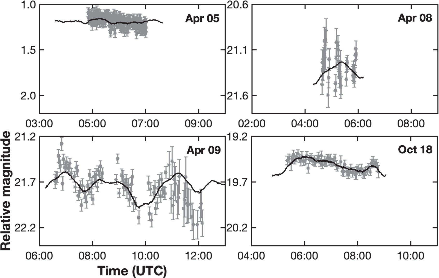
Figure 4. 2018 EB optical lightcurves with photometry reported as relative magnitudes. The horizontal and vertical axes have the same dimensions for all panels: 7 hr and 1.2 mag. The shape model fits to the lightcurves (in black) are discussed in Section 4.3.
Download figure:
Standard image High-resolution imageTable 2. Master Log of Optical Observations in 2018
| Date | Time (UTC) | R.A. | Decl. | Apmag | Distance | SOT | STO | TOM | Illu. | Filters | Obs. |
|---|---|---|---|---|---|---|---|---|---|---|---|
| START STOP | (deg) | (deg) | (mag) | (au) | (deg) | (deg) | (deg) | (%) | |||
| Apr 5 | 04:51:16 07:01:50 | 219.2 | 8.1 | 15.3 | 0.027 | 151.1 | 28.1 | 40.5 | 77.6 | Clear | 807 |
| Apr 8 | 04:39:02 05:56:14 | 223.6 | 45.5 | 17.0 | 0.041 | 122.2 | 55.9 | 87.9 | 51.0 | Clear | U82 |
| Apr 9 | 06:36:14 12:08:56 | 225.1 | 53.0 | 17.6 | 0.049 | 115.2 | 62.3 | 97.9 | 40.1 | Clear | U82 |
| Oct 18 | 05:21:00 08:47:41 | 85.8 | −59.5 | 19.8 | 0.105 | 94.9 | 79.2 | 37.5 | 64.5 | W | W85 |
| Oct 19 | 07:03:18 07:38:31 | 85.4 | −61.1 | 19.9 | 0.113 | 94.3 | 79.3 | 89.5 | 73.5 | g', i', z' | I33 |
Note. The times show the start and stop times for each optical data set. October 19 observations were used for broadband colors as opposed to lightcurves. R.A. and decl. are the ICRF astrometric R.A. and decl. of 2018 EB at the mid-epoch of the observations. We also list the asteroid's approximate apparent visual magnitude (Apmag), distance from Earth in au, Sun–observer–target (SOT) angle, Sun–target–observer (STO) angle, target–observer–Moon (TOM) angle, and percentage of the Moon's illumination (Illu.) as listed on JPL's Horizons online solar system data and ephemeris computation service (Giorgini et al. 1997). The last two columns show the filters used in the observations and the International Astronomical Union codes for the observing sites: 807—Cerro Tololo Observatory, La Serena, Chile; U82—CS3–Palmer Divide Station, Landers, USA; W85—Cerro Tololo–LCO A, Chile; and I33—SOAR, Cerro Pachon, Chile.
Download table as: ASCIITypeset image
We remeasured the April 9 lightcurve based on raw imaging data from Warner & Stephens (2019a) because the asteroid was moving very rapidly against the stellar background, and special care was needed when selecting the stars for relative photometry. We used seven sets of 10 background stars with consecutive fields being linked by three to four stars that were common to both fields. For the final 11 frames of the April 9 lightcurve, only five background stars were used due to a lack of suitable stars. Consequently, the data quality deteriorated significantly toward the end of the observing run.
2018 EB already had several rotation periods published by the time we started this analysis. Warner & Stephens (2019a) reported periods of 6.32 hr and 3.16 hr based on a preliminary photometry reduction. However, our radar data do not support these two values. A radar-estimated diameter of ∼320 m in combination with a 6.32 hr period would produce a ∼30% narrower Doppler frequency bandwidth than reported in Table 4 (see Equation (1)). Alternatively, a ∼320 m-sized object in combination with a 3.16 hr period would produce ∼30% wider bandwidths than reported in Table 4. Our radar line of sight would have to be ∼45° on all observing days in order to produce the observed ∼2 Hz bandwidths. A similar argument applies to the even more rapid period of 2.600 ± 0.437 hr reported in Borisov et al. (2021).
All lightcurves used in this analysis are shown in Figure 4, and their raw data are listed in Table 3. We initially attempted to fit the April 9 lightcurve with the second-order Fourier series in Matlab, and we obtained a range of rotation periods from 4.1 to 4.8 hr. This was consistent with the radar-derived period based on the bandwidth of the primary (Section 2.1). These preliminary period estimates were useful cross-checks for the period obtained from the shape modeling analysis described in Section 4.
Table 3. Optical Lightcurves of the Asteroid 2018 EB
| JD | Mag. | Δmag | Obs. | ID |
|---|---|---|---|---|
| (days) | (mag) | (mag) | ||
| 2458213.702280 | 1.088 | 0.050 | 807 | 1 |
| 2458213.702593 | 1.091 | 0.050 | 807 | 1 |
| 2458213.702905 | 1.160 | 0.050 | 807 | 1 |
| 2458213.703218 | 1.148 | 0.050 | 807 | 1 |
| 2458213.703542 | 1.128 | 0.050 | 807 | 1 |
Note. Raw data representing lightcurves in Figure 4. We list the Julian date of observation (JD), relative magnitude (Mag.), error on the magnitude measurement (Δmag), observatory that obtained the lightcurve (Obs.), and lightcurve ID (for each of the four observing dates).
Only a portion of this table is shown here to demonstrate its form and content. A machine-readable version of the full table is available.
Download table as: DataTypeset image
2.3. Visible-wavelength Spectrophotometry
We obtained broadband colors of 2018 EB with the Sloan Digital Sky Survey g', i' and z' filters on 2018 October 19 using the SOAR Telescope Goodman Spectrograph and Imager (Table 2). Conditions were mostly clear, with moderate winds (30 km hr−1) and below average seeing (around 2''). All exposures were 15 s with the telescope tracked at sidereal rates. In the , and filters, a total of 14, 20, and 26 images were taken. The exposures were taken in alternating sequences of . Images were processed using standard flat-field and bias-correction techniques. The photometry on each image was measured using the Photometry Pipeline (Mommert 2017) and a fixed aperture radius of 6 pixels (1 8) for the - and -band images and 5 pixels (15) for the band. Photometric calibration on each frame was achieved by referencing to ∼five on-chip field stars with approximately solar-like colors from the SkyMapper DR1 catalog (Wolf et al. 2018).


The images for photometry were taken over a span of about 30 minutes, a nonnegligible fraction of the estimated ∼4 hr rotation period for the primary but not long enough to improve period determination. We use images with the highest signal-to-noise, taken in the band, to account for lightcurve variability when computing colors from nonsimultaneous images. The full sequence of 20 -band images was linearly fit, showing a small ∼0.05 mag change over about 30 minutes. This functional fit to the -band data enabled computation of and colors at the times corresponding to each individual - and -band image. The final colors, = 0.72 ± 0.05 and = 0.04 ± 0.10, thus represent the weighted mean of all individual measurements with uncertainties presented as the standard deviation of all values for a given color. These reflectance values were then compared to each classification in the Bus taxonomic system (Bus & Binzel 2002). The formal best fit is the Xk-type (rms = 0.02). The envelopes for other less likely taxonomic types are shown in Figure 5, including S-type (rms = 0.07) and C-type (rms = 0.09).


Figure 5. The measured colors are = 0.72 ± 0.05 and = 0.04 ± 0.10. The best-fit taxonomic type in terms of minimum rms is an Xk-type. The envelopes for S and C taxonomic types are also shown.


Download figure:
Standard image High-resolution image3. Satellite
3.1. Radar Detection
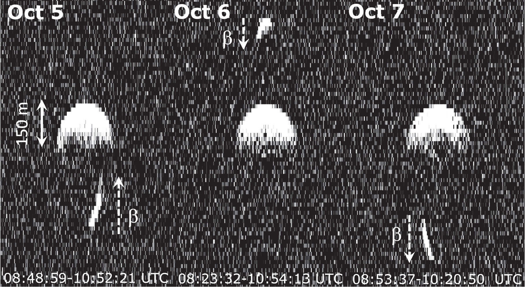
The satellite was first detected during relatively coarse-resolution delay-Doppler imaging in April at Goldstone (Figure 1). In October, Arecibo achieved S/Ns 12 times stronger than those at Goldstone in April, and the echo from the satellite was clearly visible. Figure 6 shows the daily sums that display the motion of the satellite in its orbit about the primary. The maximum projected separation in range between the satellite and the primary centers of mass increased from ∼300 m to ∼390 m between October 6 and 7 and is consistent with a radar line of sight that was approaching the mutual orbit plane. The satellite was also detected in the echo power spectra and imaging data at Goldstone from October 5 to 9. The S/Ns at Goldstone were sufficient for detection of the satellite, but we did not obtain any detailed imaging. The satellite went into a radar eclipse downrange from the primary on October 7 while we observed from Goldstone. Observations at Arecibo ended just as the satellite was approaching its maximum separation behind the primary, but Goldstone continued to observe for another 3 hr. We detected the satellite echo in CW observations until about 10:30 UTC (Figure 7), but the echo disappeared until ∼12:00 UTC from 75 m imaging data (Figure 8). We initially attributed this to low S/Ns, but we later realized that the more likely explanation was a radar eclipse.

Figure 6. Arecibo daily sums of delay-Doppler images. Time delay and Doppler frequency follow the same convention described in Figure 1. The range resolution is 0.1 μs for all panels. The Doppler frequency resolutions are 0.029 Hz on October 5 and 0.031 Hz on October 6 and 7. These frequency resolutions yielded one look per run. The number of looks in each image are 80, 104, and 55, respectively. The panel dimensions are 7 μs (1050 m) × 6.2 Hz. Ephemeris drift was removed with a first-order polynomial. The contrast was adjusted to highlight the satellite (marked as β), resulting in saturation of the echo of the primary. Dashed white arrows indicate the direction of the satellite's motion.
Download figure:
Standard image High-resolution image
Figure 7. Goldstone detections of the satellite in OC echo power spectra obtained on October 7. The satellite was approaching its maximum separation from the primary downrange and was about to enter an eclipse. The Doppler frequency resolution is 0.5 Hz (X band), and we list the midtimes of each weighted sum of 15 runs.
Download figure:
Standard image High-resolution image
Figure 8. Goldstone images of the satellite emerging from a radar eclipse downrange from the primary on October 7. Delay-Doppler image resolution is 0.25 μs × 0.51 Hz (X band), and each image is a weighted sum of 20 runs with 10 runs in overlap. The midtimes of each image are listed.
Download figure:
Standard image High-resolution imageFigure 9 shows echoes from the satellite obtained at Arecibo on October 5–7. We processed the data so that they have one look per run and thus the finest possible Doppler frequency resolution of 0.029 Hz on October 5 and 0.031 Hz resolution on October 6–7. We summed 20 runs, spanning ∼28 minutes, to create a single delay-Doppler image. We used a second-order polynomial, p0 + p1 t + p2 t2, where t is time and pi are the coefficients, to correct for the satellite's motion in range and Doppler frequency when summing the data from different runs. In this shift-and-stack technique, the polynomial accounts for both the drift due to orbital motion and the small drift due to the imperfect ephemeris of the system. Naidu et al. (2020) used to correct for orbital motion of the satellite of (65803) Didymos, but given the short data arcs and the additional drift due to ephemeris corrections, we found it sufficient to use a polynomial.

Figure 9. Arecibo delay-Doppler images of the satellite. The Doppler frequency resolutions are 0.029 Hz on October 5 and 0.031 Hz on October 6 and 7. The range resolution is 0.1 μs (15 m). All frames have the same vertical and horizontal dimensions, 450 m × 1.25 Hz. Each frame represents a sum of 20 runs (∼28 minutes of data integration), except the last image on October 7, which is a sum of 15 runs (∼22 minutes of data integration). Midtimes of the sums in UTC are provided for each panel. The satellite motion and the ephemeris drift were removed with a second-order polynomial, so that the satellite remains in the same range location in the sums. The contrast was saturated at the 3σ level.
Download figure:
Standard image High-resolution imageWe estimated the visible extent and Doppler bandwidth for the satellite by counting contiguous pixels above 3σ signal strength (Table 4). The uncertainties in Table 4 include our considerations of the delay-Doppler imaging resolution, image quality, and number of looks. The average visible extent on October 7 (∼66 m) appears to be slightly less than observed on October 5 and 6 (∼80 m), hinting that the object could be somewhat elongated. We also searched for bandwidth changes in the individual images on October 5 and 7 because there was substantial orbital motion between the first and last images. However, the S/Ns dropped significantly from the first to the last frame on each day as 2018 EB was setting at Arecibo. We can report only tentative evidence that the bandwidth narrowed by one Doppler frequency bin on October 7, but the S/Ns in the frames are weak, so a search for bandwidth changes in the satellite was inconclusive.
Table 4. S-band Doppler Frequency Bandwidths, Visible Range Extents, and Estimated Rotation Periods for the Primary and the Satellite
| Date | Obs. | Data | S Bandwidth | Δf | Visible Extent | Δd | Pr. |
|---|---|---|---|---|---|---|---|
| (Hz) | (Hz) | (m) | (m) | (hr) | |||
| Primary | |||||||
| Apr 7 | G | Doppler | 1.69 | 0.50 | ⋯ | ⋯ | ⋯ |
| Oct 5 | G | Doppler | 1.96 | 0.50 | ⋯ | ⋯ | ⋯ |
| Oct 6 | G | Doppler | 2.16 | 0.50 | ⋯ | ⋯ | ⋯ |
| Oct 7 | G | Doppler | 2.17 | 0.50 | ⋯ | ⋯ | ⋯ |
| Oct 8 | G | Doppler | 1.91 | 0.50 | ⋯ | ⋯ | ⋯ |
| Oct 9 | G | Doppler | 1.95 | 0.50 | ⋯ | ⋯ | ⋯ |
| Oct 5 | A | Doppler | 2.03 | 0.09 | ⋯ | ⋯ | ⋯ |
| Oct 6 | A | Doppler | 2.21 | 0.09 | ⋯ | ⋯ | ⋯ |
| Oct 7 | A | Doppler | 2.35 | 0.09 | ⋯ | ⋯ | ⋯ |
| Oct 5 | A | Imaging | 1.89 ± 0.12 | 0.12 | 156 ± 30 | 15 | 4.6 ± 0.9 |
| Oct 6 | A | Imaging | 2.09 ± 0.09 | 0.09 | 153 ± 30 | 15 | 4.1 ± 0.8 |
| Oct 7 | A | Imaging | 2.15 ± 0.09 | 0.09 | 166 ± 30 | 15 | 4.3 ± 0.8 |
| Satellite | |||||||
| Oct 5 | A | Imaging | 0.25 ± 0.03 | 0.03 | 80 ± 30 | 15 | 17.8 ± 7.0 |
| Oct 6 | A | Imaging | 0.26 ± 0.03 | 0.03 | 78 ± 30 | 15 | 16.7 ± 6.7 |
| Oct 7 | A | Imaging | 0.24 ± 0.03 | 0.03 | 66 ± 30 | 15 | 15.3 ± 7.2 |
Note. Lower bounds on the Doppler frequency bandwidths of the echo power spectra shown in Figure 2. The observatory site column (Obs.) indicates data obtained at Goldstone (G) or Arecibo (A). We measured the bandwidths 3σ above the noise floor. All Goldstone bandwidth measurements were converted from the X band to the S band. The October 9 bandwidth was estimated at 1σ due to low S/Ns at Goldstone. We also list the average delay-Doppler dimensions of the primary and the satellite based on Arecibo images. The averages were calculated based on visual measurements of the 10-run sums for the primary and the 20-run sums for the satellite. We counted contiguous pixels that are at least 3σ above the noise level. Rotational periods were calculated based on Equation (1), and they assume an equatorial view. The period uncertainties were calculated by propagating the errors in bandwidth and diameter.
Download table as: ASCIITypeset image
If we double the mean visible extent for the satellite from Table 4, then we obtain a zeroth-order diameter estimate of ∼150 m. It is unlikely that the volume of the satellite is much larger than implied by this diameter, but the volume could be smaller if the shape is flattened, like the satellites of (66391) Moshup (1999 KW4) (Ostro et al. 2006), (153591) 2001 SN263 (Becker et al. 2015), and Didymos (Daly et al. 2023). We thus assign an uncertainty of m on the equivalent diameter for the satellite. These error bars account for the data resolution and S/Ns and are necessarily subjective. More precise estimates would require shape modeling, but the images do not have sufficient rotational coverage, S/Ns, or resolution. A satellite with a diameter of ∼150 m is relatively large for a primary ∼320 m in diameter, but systems with Ds /Dp ∼ 0.5 have been observed before: (66063) 1998 RO1 (Pravec et al. 2016), (85938) 1999 DJ4 (Pravec et al. 2006), (385186) 1994 AW1 (Richardson et al. 2015), (494658) 2000 UG11 (Pravec et al. 2006), 2003 SS84 (Nolan et al. 2003a), and (410777) 2009 FD (Naidu et al. 2015b). We used Equation (1), the mean bandwidths, and the estimated diameters from Table 4 in order to constrain the rotation period of the satellite. If we assume that the subradar latitudes were close to equatorial, then this simplified approach suggests that the satellite has a rotation period of 17 ± 4 hr.

3.2. Satellite Orbit Determination
For radar observations, the satellite's orbit is typically determined using measurements of range-Doppler separations between the satellite's center of mass (COM) and that of the primary over time (Margot et al. 2002; Ostro et al. 2006; Shepard et al. 2006; Fang et al. 2011). The COM for both objects generally lies near the middle of the trailing edge of their respective radar echoes.
The COMs for the primary and the satellite can be obtained from shape models, and they can also be estimated visually. We did not have a shape model for the satellite due to its small size and unresolved radar images, so we estimated the location of its COM visually. The COM of the primary was estimated via shape model. This shape model was developed at the initial stage of this analysis and used for the orbit fit. However, it became apparent that the orbital fitting part provided a good constraint on the orbital pole and presumably the pole of the primary, which led to reevaluation and another iteration of the entire shape modeling process. We start by describing the orbital fit procedure first, followed by the shape modeling with an understanding that we went through "shape model–orbit fit–shape model" iterations. The differences in the COM estimates for the primary between the starting and final shape models were within the errors assigned to the range and Doppler separations between the satellite's and the primary's COMs listed in Table 5. We assigned uncertainties based on data resolution, S/Ns, and our subjective sense about data quality. The most precise measurements, with errors of 30 m in range and 0.1 Hz in Doppler frequency, were obtained at Arecibo on October 5–7. The data obtained at Goldstone on October 8–9 had significantly larger uncertainties due to the lower S/Ns and coarser resolutions but were still valuable because they sampled different orbital geometries as the asteroid traversed the sky. In the case of 2018 EB, we also observed a radar eclipse, and the timing of this event can also be utilized in orbit fitting.
Table 5. Relative Radar Astrometry for the Satellite
| Date | Midtime | OR | 1σR | OD | 1σD | CR | CD | wt. residR | wt. residD | Obs. |
|---|---|---|---|---|---|---|---|---|---|---|
| (UTC) | (hh:mm:ss) | (m) | (m) | (Hz) | (Hz) | (m) | (Hz) | |||
| Oct 5 | 08:31:52 | ⋯ | ⋯ | 0.09 | 0.11 | ⋯ | 0.08 | ⋯ | 0.12 | A |
| Oct 5 | 08:32:51 | ⋯ | ⋯ | 0.09 | 0.14 | ⋯ | 0.08 | ⋯ | 0.07 | G |
| Oct 5 | 08:39:01 | ⋯ | ⋯ | 0.12 | 0.11 | ⋯ | 0.11 | ... | 0.09 | A |
| Oct 5 | 08:47:11 | ⋯ | ⋯ | 0.14 | 0.14 | ⋯ | 0.15 | ... | −0.06 | G |
| Oct 5 | 08:51:18 | 268 | 30 | 0.14 | 0.10 | 283. | 0.17 | −0.48 | −0.28 | A |
| Oct 5 | 08:55:53 | 271 | 30 | 0.17 | 0.10 | 280. | 0.19 | −0.29 | −0.19 | A |
| Oct 5 | 09:00:11 | 279 | 30 | 0.19 | 0.10 | 277. | 0.21 | 0.06 | −0.19 | A |
| Oct 5 | 09:01:31 | ⋯ | ⋯ | 0.23 | 0.14 | 276. | 0.21 | 0.00 | 0.11 | G |
| Oct 5 | 09:04:29 | 277 | 30 | 0.27 | 0.10 | 274. | 0.23 | 0.10 | 0.42 | A |
| Oct 5 | 09:08:47 | 280 | 30 | 0.24 | 0.10 | 270. | 0.25 | 0.35 | −0.08 | A |
| Oct 5 | 09:13:05 | 269 | 30 | 0.27 | 0.10 | 266. | 0.27 | 0.12 | 0.03 | A |
| Oct 5 | 09:17:23 | 253 | 30 | 0.32 | 0.10 | 262. | 0.29 | −0.30 | 0.34 | A |
| Oct 5 | 09:21:53 | 253 | 30 | 0.24 | 0.10 | 257. | 0.31 | −0.12 | −0.65 | A |
| Oct 5 | 09:26:36 | 247 | 30 | 0.27 | 0.10 | 251. | 0.33 | −0.14 | −0.55 | A |
| Oct 5 | 09:30:54 | 247 | 30 | 0.27 | 0.10 | 246. | 0.34 | 0.03 | −0.73 | A |
| Oct 5 | 09:35:23 | 243 | 30 | 0.36 | 0.10 | 240. | 0.36 | 0.09 | −0.01 | A |
| Oct 5 | 09:40:04 | 227 | 30 | 0.34 | 0.10 | 234. | 0.38 | −0.23 | -0.40 | A |
Note. Range is the distance between the satellite's COM and the primary's COM. OR is the observed range offset, and CR is the computed offset calculated based on our preferred orbit fit. Negative distances indicate that the satellite is closer to the observer than the primary, and positive distances indicate the satellite is farther from the observer. Doppler frequency is the offset in Doppler frequency between the COMs of the primary and the satellite. Goldstone X-band frequency measurements were converted to the S band. A and G correspond to Arecibo and Goldstone. OD is the observed offset in Doppler frequency, and CD is the calculated offset. The observed uncertainties, 1σR and 1σD , were assigned based on the data resolutions and a subjective estimate of the data quality. We also list residuals normalized by their weights.
Only a portion of this table is shown here to demonstrate its form and content. A machine-readable version of the full table is available.
Download table as: DataTypeset image
The orbital fit was a two-step process: the first step initialized the Keplerian orbital elements, and the second step optimized these elements via the downhill simplex method (Press et al. 1992). We used six Keplerian elements to fit the data: semimajor axis a, eccentricity e, inclination i, mean anomaly at the epoch M, argument of periapsis ω, and longitude of the ascending node Ω. The semimajor axis was initialized between 0.40 and 0.55 km in steps of 0.01 km. This range was chosen because of the measured separations in Table 5. The starting orbits were circular, e = 0. The inclination was initialized from 0° to 180° in steps of 5° with respect to the International Celestial Reference Frame (ICRF). The mean anomaly and the node were initialized from 0° to 360° in steps of 10°. The system mass was initialized for a sphere with a radius of 0.15 km and a density between 0.5 and 2.2 g cm−3 in steps of 0.1 g cm−3. We used an upper bound of 2.2 g cm−3 because the NEA binary and triple systems for which densities are available, namely, (66391) Moshup (Ostro et al. 2006), (136617) 1994 CC (Brozović et al. 2011), (153591) 2001 SN263 (Becker et al. 2015), (185851) 2000 DP107 (Naidu et al. 2015a), and (276049) 2002 CE26 (Shepard et al. 2006), all have densities less than 2 g cm−3.
Each starting set of orbital elements was converted into a state vector in the Cartesian coordinates (x0, y0, z0, vx0, vy0, vz0) with the COM of the primary at the origin and referenced to the ICRF. The state vector was propagated in time via conic theory (Goodyear 1965) and converted into radar observables, time delay, and Doppler frequency separations from the primary. We also calculated separations between the satellite and the primary in the plane of the sky in order to evaluate conditions for the radar eclipse on October 7. We defined the plane-of-sky separation d as

where is the position vector from the observer to the primary's center and is the position vector from the observer to the satellite's center (Aksnes 1974). The conditions for radar eclipse occur if d < R1 + R2, where R1 and R2 are radii for the primary and the satellite (assumed 150 m and 75 m), and if . We calculated the separation value d for the start and stop times of the eclipse, 10:30 UTC and 12:00 UTC, and kept all combinations of orbital elements that resulted in d within 50% of R1 + R2. This corresponds to 30–40 minutes uncertainty on the start–stop times, which is a conservative 3σ estimate given the weak data in Figure 8. The "eclipse score" for the fit was calculated as (d − (R1 + R2))/(R1 + R2). For the "perfect" correspondence to the observed start–stop times, we would get zero for both ingress and egress.


A 7D simplex search was used to adjust the initial state vector of the satellite and the nominal system mass, aiming to find a solution with the lowest rms of the residuals. The final state vector was converted back into Keplerian elements. We also converted pole directions from R.A. and decl. to the ecliptic longitude and latitude. We kept solutions with e < 0.2, 0.4 < a < 0.55 km, and an rms of the residuals ≤1. Figures 10 and 11 show the final distribution of the orbital parameters for 950 candidates. The possible orbit poles occupy a narrow swath across the sky. The prograde poles have a noticeable clumping of candidates around the longitude and latitude (90°, 45°). We further constrained the candidate region by selecting for the solutions that have an overall rms of the residuals of ≤0.7 and an eclipse score of ≤0.2. The final 116 candidates marked in orange in Figure 10 are all in the prograde direction. Furthermore, 87% are in the region of 80°–100° in longitude and 40°–50° in latitude. Table 5 shows delay and Doppler residuals for the best solution: orbit pole at λ = 93° and β = 48°, a = 0.50 km, e = 0.15, system mass M = 2.03 × 10¹⁰ kg, and P = 16.85 hr. We used the bounds set by the final 116 candidates to write a more general orbit solution: km, e = 0.15 ± 0.04, kg, and hr. We note that the nominal orbit has a significant eccentricity, like the orbits of (164121) 2003 YT1 (Nolan et al. 2004), (311066) 2004 DC (Taylor et al. 2008), and (153958) 2002 AM31 (Taylor et al. 2013). No solutions were found for e ≤ 0.05, and the residuals were significantly worse for the solutions where we forced e ∼ 0.1. Eccentricity introduces a possibility of apsidal precession for the oblique shape of the primary. However, we cannot determine the precession rate because the radar data arc is too short (October 5–9), and the data are too coarse. With the current uncertainty on the orbit period, we do not know how many full revolutions have occurred between April and October.


Figure 10. Results of the orbital pole search for the satellite with respect to ecliptic longitude and latitude. Gray circles represent χ2 values of the 950 candidates. Darker color corresponds to solutions with lower χ2 (see color bar on the far right). Orange circles mark 116 candidates with a radar eclipse score of <0.2.
Download figure:
Standard image High-resolution image
Figure 11. Results of the search for the best combinations χ2-wise of the semimajor axis, eccentricity, system mass, and period. The rest of the caption is the same as in Figure 10.
Download figure:
Standard image High-resolution image4. Shape Modeling
We used the Shape software (Hudson 1994; Magri et al. 2007) to estimate the 3D shape and spin state of the 2018 EB primary. The modeling was done using the delay-Doppler images, echo power spectra, and optical lightcurves. The Shape algorithm uses a weighted least-squares minimization process to find the best solution. The cost function is a reduced χ2 score, calculated by dividing the sum of the weighted residuals by the number of data points, plus a series of "penalty" functions intended to regularize the fit by suppressing nonphysical results. The shape modeling progressed in stages. We started by approximating the shape of 2018 EB with a sphere. Our goal was to constrain its size, rotation period, and pole direction. The second stage of modeling was done with a more sophisticated model that parameterized the shape with the eighth-degree spherical harmonics series. In the final stages of the fit, the model was approximated as a 3D mesh made of triangular facets.
The modeling was guided by careful consideration of the initial parameters and the weights assigned to the penalty functions. The penalty functions were chosen to prevent departures from principal-axis rotation and uniform internal density. For example, the "inertiadev_uni" penalty is mathematically defined as , where the first vector components are the diagonal elements of the uniform-density inertia tensor divided by the square root of the sum of the squares of all nine tensor elements, and the second vector is the unit vector calculated from the three dynamical principal moments of inertia. The resulting penalty function is zero if these two vectors are identical, and it is positive for any other case, which means the function pushes the model toward principal-axis rotation with the three principal inertia axes aligned with the three body-fixed coordinate axes. The penalty function is added directly to the final χ2 value, and we scale its contribution by a weighting factor to adjust its influence on the fit. The penalty functions also prevented the object's volume from growing larger than the volume of a 340 m diameter sphere, discouraged facet-scale topographic spikes that have an unphysical appearance, and penalized small-scale concavities. We adjusted penalty weights until we obtained the best possible match between the fits and the data.

4.1. Data Set Used in Shape Modeling
Our modeling data set contained weighted contributions from lightcurves, echo power spectra, and delay-Doppler images. The radar data consisted of 23 Goldstone echo power spectra, four Arecibo echo power spectra, and 48 delay-Doppler images from Arecibo. We removed the satellite echoes from the echo power spectra by interpolating between the adjacent Doppler bins. The satellite was removed from the imaging data by using masking files consisting of binary pixel values: zeros and ones. If the image pixel is multiplied by a masking pixel with a value of 0, it does not contribute to the fit. The OC power spectra and delay-Doppler images obtained at Arecibo on October 5–7 contained up to 7 minutes of rotation by the primary. Our intention was to average as little rotation as possible in order to keep the features sharp while maintaining good noise statistics and reasonably strong S/Ns. If we assume that the primary's rotation period is ∼4 hr, then 7 minutes corresponds to ∼10° of rotation.
The Goldstone echo power spectra, although weaker than the Arecibo data, were important for the modeling because they constrained the bandwidth of the primary and the pole direction on 3 days without Arecibo observations: April 7, October 8, and October 9. On April 7, we summed ∼7 minutes of CW data, equivalent to about 10° of rotation. For CW data acquired at Goldstone in October, we summed ∼20 minutes of data due to low S/Ns, which introduced ∼30° of rotational smear. To help model data with this much rotation, we used Shape to synthesize five instantaneous echo power spectra from the model separated in time by only a few minutes (e.g., 240 s on October 6). These spectra were then averaged to obtain a single, rotationally smeared model spectrum that was compared with the data.
4.2. Shape Modeling of the Primary
The primary appeared to be a symmetric object without pronounced surface features. As such, a sphere was a reasonable starting approximation for its shape. We sampled diameters between 0.28 and 0.36 km, with increments of 0.02 km. We conducted a grid search across the entire sky in order to constrain the pole direction. The ecliptic longitudes (λ) and latitudes (β) were sampled uniformly in the steps of 5°. We sampled rotation rates from 1800° to 2500° day−1 (3.5–4.8 hr) in steps of 20° day−1 based on the period constraints we discussed in Sections 2.1 and 2.2. The fit quality was evaluated based on χ2 value for each (fixed) combination of size, period, and pole direction. The initial shape modeling data set contained delay-Doppler and Doppler-only data weighted so that they contributed 64% and 36% to the χ2 value, respectively. We did not use lightcurves at this stage of the modeling because the shapes were approximated as spheres. The preliminary results showed a preference toward diameters D > 0.30 km and periods 3.9 hr < P < 4.5 hr. All size and period combinations showed a χ2 minimum in the pole region represented by the dark swaths in Figure 12. This region encompassed the orbital pole constraint from Figure 10.

Figure 12. Constraints on the pole direction for the primary from shape modeling. The shape was approximated with a sphere with diameter of 320 m. The χ2 value is mapped for all ecliptic longitudes and latitudes. The white regions represent large values of χ2 where the fits are poor. The dark regions represent admissible χ2 values where the fits match the delay-Doppler and Doppler-only data. The crosses mark the observer-centered longitude and latitude at the time of radar (blue) and lightcurve (red) observations. We also show the locations of the heliocentric orbit pole (HOP) for the system, the nominal satellite's orbit pole (SOP), and nominal pole of the primary (PP).
Download figure:
Standard image High-resolution imageIn the second stage of modeling, we used the eighth-degree spherical harmonics to represent the shape of the primary. Given that the first stage of modeling did not significantly constrain the pole direction, and considering that it is reasonable to assume that the satellite's orbit pole corresponds to the pole of the primary, we adopted 10 poles from the orange region in Figure 11 as candidates: (50°, 35°), (60°, 40°), (70°, 40°), (70°, 45°), (80°, 45°), (90°, 45°), (90°, 50°), (100°, 45°), (110°, 40°), and (120°, 35°). We initialized spin rates from 1300° to 4600° day−1 in steps of 20° day−1 (1.9–6.6 hr period). We used a wider period search than we did initially because we now included the lightcurves, and we wanted to test more rigorously if slower or more rapid periods are possible. Figure 13 shows how the χ2 varied with the spin rate. We show individual χ2 contributions from the CW data because these data cover the entire radar observing campaign (April 7, October 5–9), and they are less noisy than the delay-Doppler images. We note that the χ2 remains relatively flat for a large span of spin rates. The preferred rotation rate occurs around 2000° day−1 (P ∼ 4.3 hr), similar to our findings from Sections 2.1 and 2.2. The overall χ2 with contributions from CW, delay-Doppler images, and lightcurves shows a similar trend. The inclusion of lightcurves resulted in the steeper slope in χ2, selecting for less rapid rotation rates. Nolan et al. (2013) pointed out that the standard statistical definition of a 1σ error (e.g., Bevington & Robinson 2003) based on the curvature of the calculated χ2 produces "unreasonably large values" because the fit cannot distinguish between contributions from the signal and from the background noise. Thus, we visually inspected the various models and found that 1σ errors (fits noticeably less good than the best-fit model) roughly corresponded to a 10% increase in χ2. We adopted day−1 as a possible range of spin rates/periods. We also show in the last panel of Figure 13 that the overall χ2 remained almost flat with respect to our 10 candidate poles. This means that we can select any of these candidate poles as "nominal." While it is not unusual to have a relatively unconstrained or prograde/retrograde ambiguous pole (Hudson & Ostro 1994; Busch et al. 2007; Brozović et al. 2011), the rotation rate is usually constrained better than ∼14%, as we have here. 2018 EB was too small and too slow for the radar data to show obvious bandwidth changes for different period considerations, and the delay-Doppler images did not have any obvious features to track. Lightcurves were also able to accommodate a wide range of spin rates due to either noisy (April 9) or relatively flat lightcurves (April 5 and October 18). The absence of a clear period signature prevented any detailed shape modeling. However, a ∼14% constraint was sufficient to estimate the object's dimensions and to obtain general outlines of the shape. The size estimate based on the shape model is still better than the visual assessment and important for determination of the bulk density and radar and optical albedos.


Figure 13. Constraints on the rotation rate and pole direction for the primary from shape modeling. We used the eighth-degree spherical harmonics to represent the shape. (A) Reduced χ2 for the echo power spectra (CW). (B) Reduced χ2 for all data (the echo power spectra, delay-Doppler images, and lightcurves). In this example, the pole direction was held fixed at λ = 70°, β = 45°. (C) Reduced χ2 for all data for a spin rate fixed at 2000° day−1.
Download figure:
Standard image High-resolution imageWe converted the 50 best spherical harmonics models into vertex shape models with 512 vertices, 1020 triangular facets, and an effective resolution of ∼27 m. All shape and spin parameters were allowed to adjust at this point. We selected one of the models (spin rate of 2030° day−1, pole direction λ = 70°, β = 50°) as "nominal" based on its overall χ2 value and our subjective preference during a visual inspection. The nominal pole was adjusted from the initialized value of λ = 70° and β = 45°. We used all 50 vertex model finalists to calculate the 3D shape uncertainties.
4.3. Shape Modeling Fit to the Data
Figure 14 shows the Goldstone and Arecibo OC echo power spectra and their respective fits. The fits match the bandwidths and the spectral shapes. Figure 15 shows delay-Doppler data, fits, and plane-of-sky views of the nominal model. The model reproduces the bandwidths, visible extents, and echo shapes within reasonable limits given the low S/Ns of the data. The radar line of sight was ∼42° off the equator on October 5, which shrank the bandwidth by ∼26% with respect to an equatorial orientation. Hence, the echo occupied fewer pixels, and this made the data more difficult to model. The radar line of sight was ∼18° off the equator on October 7. We used the nominal spin rate (2030° day−1) to search for common features at the same longitudes in the images obtained on different days. However, although there is some overlap in coverage across multiple days, the images had different S/Ns, and we could not find common features. Figure 4 shows the lightcurves and their respective fits for the nominal pole (λ = 70°, β = 50°) and a period of 4.26 hr. The fit reproduced the nearly flat lightcurve on April 5 and a ∼6 hr lightcurve with pronounced variations on April 9. The model also matched the small-amplitude lightcurve on October 18.

Figure 14. OC echo power spectra used in the shape modeling. The data are shown as thin lines, and the data fits are shown as thick dashed lines. The spike from the satellite was removed from the data by interpolating between the adjacent bins. All spectra were normalized to have zero mean and unit standard deviation of the receiver noise. Identical linear scales are used for each panel. (A) Goldstone data (X band, 8560 MHz). Each spectrum is centered at 0 Hz and extends from −10 Hz to +10 Hz with a frequency resolution of 0.5 Hz. The vertical tick at 0 Hz shows ±1σ. (B) Arecibo data (S band, 2380 MHz). Each spectrum is centered at 0 Hz and extends from −3 Hz to +3 Hz with a frequency resolution of 0.114 Hz on October 5 and 0.094 Hz on October 6–7. The vertical tick at 0 Hz shows ±5σ.
Download figure:
Standard image High-resolution image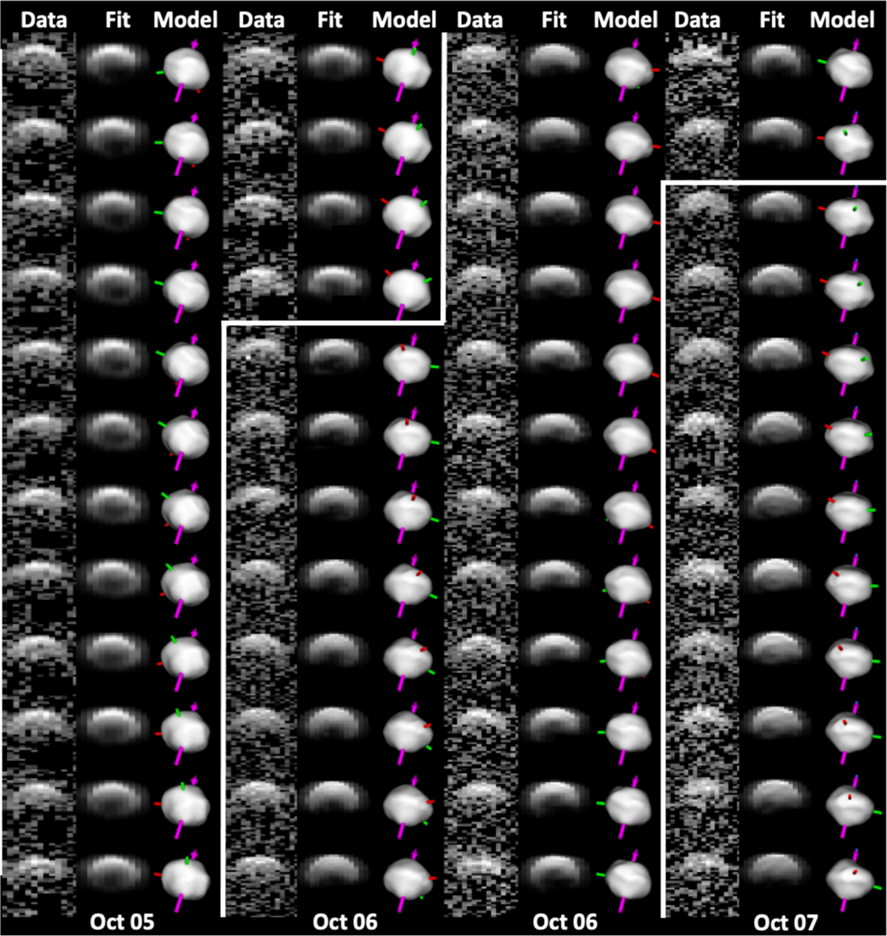
Figure 15. Collage of, from left to right, delay-Doppler radar images, the corresponding fits (synthetic images), and plane-of-sky renderings of the shape model. In the data and fits, the time delay increases from top to bottom, and the Doppler frequency increases from left to right. The plane-of-sky view is contained in a 0.5 km × 0.5 km square with 151 × 151 pixels. The magenta arrow shows the instantaneous orientation of the spin vector, and the red, green, and blue shafts denote the positive ends of the long, intermediate, and short principal axes. The dark squares in the October 5 images represent the mask that we applied to eliminate the satellite echo from shape modeling of the primary.
Download figure:
Standard image High-resolution image4.4. Size and Shape of the Primary
Figure 16 shows principal-axis views of our preferred vertex model. The model resolution (∼27 m) was coarser than the delay-Doppler imaging resolution of 15 m, but it was sufficient to describe the data at hand. We also had a relatively large uncertainty on the rotation period, which prevented any detailed modeling of the shape features. The radar images and lightcurves provided nearly complete coverage. The overall shape is somewhat more subdued and more oblate than the toplike shapes of other binaries such as Moshup (Ostro et al. 2006). However, not all primaries modeled to date have a prominent equatorial bulge. For example, the primary of 2002 CE26 had a relatively rounded appearance (Shepard et al. 2006), and the shape of Didymos, as observed by the DART spacecraft, also appeared oblate with a less pronounced equatorial bulge (Daly et al. 2023). The 2018 EB model has principal-axis dimensions of X = 0.34 ± 0.04 km, Y = 0.33 ± 0.04 km, and Z = 0.29 ± 0.04 km and an equivalent diameter of 0.30 ± 0.04 km. We define the equivalent diameter as the diameter of a sphere that has the same volume as the model. Our equivalent diameter is somewhat larger than the NEOWISE estimate of D = 0.23 ± 0.07 km (Masiero et al. 2020), but the diameters are consistent within their uncertainties. Size variations among the final 50 vertex shape models were much smaller than the uncertainties listed in Table 6. We adopted ∼10% uncertainties on the X and Y principal dimensions to account for the data resolution and unmodeled sources of errors. We also checked these uncertainties by manually scaling the size of each axis. Shape models estimated from inversion of radar data are known to have larger uncertainties on the short principal axis (Hudson & Ostro 1999), especially when the observations are confined to nearly equatorial subradar latitudes. However, we observed 2018 EB at −42° in subradar latitude on October 5 and at +4° on October 9. This relatively large range of subradar latitudes allowed us to adopt the Z-axis uncertainty of 15%. Lightcurves from April 5 and 9 and October 11 also contributed to the constraints on the axis ratios.

Figure 16. Principal-axis views of the nominal 2018 EB primary shape model. The model is constructed from 512 vertices that form 1020 triangular facets and has a resolution of ∼27 m. The yellow patch in the +Z view indicates a small surface area that was not well constrained by the data. The model has the principal-axis extents of 0.34 × 0.33 × 0.29 km.
Download figure:
Standard image High-resolution imageTable 6. Physical Properties of the Primary
| Parameter | Value |
|---|---|
| Pole direction | |
| λ | 70° |
| β | 50° |
| Principal axes | |
| X | 0.34 ± 0.04 km |
| Y | 0.33 ± 0.04 km |
| Z | 0.29 ± 0.04 km |
| Axis ratios | |
| X/Y | 1.03 ± 0.17 |
| Y/Z | 1.14 ± 0.21 |
| Equivalent diameter | 0.30 ± 0.04 km |
| Surface area | 0.30 ± 0.08 km2 |
| Volume | 0.015 ± 0.006 km3 |
| DEEVE | |
| X | 0.33 ± 0.04 km |
| Y | 0.33 ± 0.04 km |
| Z | 0.26 ± 0.04 km |
| Rotation period | hr |
| Optical albedo | pV = 0.028 ± 0.016 |

Note. Physical parameters obtained from shape modeling. The prograde model was treated as nominal based on the orbital fit preference for the prograde pole solution. We adopt the orange region in Figure 10 as the pole uncertainty. Uncertainties in the physical dimensions were determined based on statistical variations among 50 shape model candidates and by considering the imaging data resolution. "DEEVE" stands for dynamically equivalent, equal volume ellipsoid. The optical albedo was calculated from the absolute magnitude 21.9 ± 0.5 and the effective diameter of the system (Deff = 0.33 ± 0.05 km; see Section 5).
Download table as: ASCIITypeset image
The nominal model of the primary has a small elongation of ∼3%, although within the uncertainties, models with higher elongations are possible. In the analysis above, we noted that the echo bandwidth varied by ∼12% as the object rotated during imaging. However, the S/Ns were relatively weak and could have contributed to the bandwidth variations. The 12% corresponds to only two Doppler frequency bins in the images. We also note that the April 5 lightcurve was almost flat during 2 hr of observations. We initially did not know if this was due to low shape elongation, a nearly pole-on view, or a period longer than a few hours. After the shape modeling, we realized that the lightcurve was obtained in a nearly equatorial view from the Earth (+15° body-fixed latitude) with an almost fully lit surface (<15% of the surface was shadowed). Thus, this lightcurve is consistent with a low elongation of the primary.
5. Optical Albedo
We estimated the visual geometric albedo using the expression pV = (1329/D)210−0.4H (Pravec & Harris 2007), where H is the absolute visual magnitude and D is the effective diameter. We adopted H = 21.9 from JPL's Small-Body Database (SBDB) 15 and a conservative 0.5 mag uncertainty (J. Giorgini, personal communication). We included contributions from the primary and satellite to compute the effective diameter of the system: Dp = 0.3 km, Ds = 0.15 km, Deff = 0.33 km. We also adopted the uncertainty on the effective diameter of 0.05 km in order to account for the uncertainty on the size of the satellite. The uncertainty in the absolute magnitude dominates the overall uncertainty of the optical albedo that we estimated by propagating the errors in D and H. We obtained pV = 0.028 ± 0.016, which implies that 2018 EB is optically dark. As noted in Section 2.3, spectrophotometry suggests that 2018 EB likely belongs to the Xk spectral complex in the Bus & Binzel (2002) taxonomic system. In their comparison with Tholen's (1984) definition of X-class, Bus & Binzel (2002) found that Xk-types most often map into M and C taxonomies (see their Table 4). For the case of 2018 EB, the 3% optical albedo is more consistent with C- than M-types.
6. Bulk Density and Porosity
The system mass of kg and the volumes of the primary and the satellite (0.015±0.006 km3 and 0.002 km3, respectively) yield an estimate for the bulk density of g cm−3. The dominant source of the density uncertainty is the volume of the primary. Taken at face value, the calculated density is consistent with the mean bulk density reported for C-complex asteroids (∼1.4 g cm−3; Carry 2012). Britt et al. (2002) reported a wide range of bulk densities for C-type meteorites, from 2 to 3.5 g cm−3. If we adopt a CI/CM meteorite as an analog for 2018 EB (average bulk density of ∼2.1–2.2 g cm−3; Britt et al. 2002), we obtain a porosity of ∼40%. If the density is in the realm of CV/CO/CR meteorite analogs (∼3.1 g cm−3; Britt et al. 2002), the porosity increases to ∼60%.


7. Disk-integrated Radar Properties
Table 7 lists disk-integrated properties for the 2018 EB system derived from the CW data. The mean OC radar cross sections are σOCsys = 0.024 ± 0.006 km2 at Arecibo and σOCsys = 0.019 ± 0.007 km2 at Goldstone. We assigned a 25% cross-section uncertainty for Arecibo and 35% cross-section uncertainty for Goldstone to account for systematic calibration and pointing errors. The cross-section uncertainties due to random statistical fluctuation were on the order of 10−4 km2 for Arecibo and 2 × 10⁻³ km2 for Goldstone. The echo power spectra from Arecibo clearly resolved the narrow echo from the satellite (Figure 2), which we removed by interpolating the echo power between the adjacent bins. This allowed us to estimate a cross section of km2 for the primary. Table 7 shows that the satellite makes a small contribution of ∼0.003 km2 to the overall S-band cross section. For consistency, we subtracted the S-band cross section for the satellite from the X-band estimates for the cross section of the system. This is a reasonable approach given that S-band and X-band values for radar scattering properties usually agree within their formal uncertainties (Nolan et al. 2013; Naidu et al. 2020). For the Goldstone data, we obtained km2. The OC radar albedo for the primary was calculated by dividing the OC cross section by the projected area of the shape model. We obtained mean radar albedos of at Arecibo and at Goldstone. The uncertainties account for the cross section uncertainties (25% for Arecibo and 35% for Goldstone) and for the projected area uncertainty of 27% (see Table 6). For comparison, with an average cross section of σOCsat = 0.0028 km2 and an effective diameter of 150 m, the satellite would have a radar albedo of ηOCsat = 0.17. However, if the satellite is slightly smaller, with a diameter of 120 m, its radar albedo would be 0.25, comparable to that of the primary. Radar albedos are known for several dozen NEAs, and 2018 EB fits into the top 30% of the radar-brightest NEAs (see Figure 3.3 in Ostro & Giorgini 2004). Virkki et al. (2022) reported that the global radar albedo mean for 41 NEAs was 0.21 ± 0.11.


Table 7. Disk-integrated Radar Properties of 2018 EB
| Date | UTC Time | Runs | Looks | OCsys | σOCsys | SC/OCsys | Aprim | ηOCp | |
|---|---|---|---|---|---|---|---|---|---|
| UTC | START STOP | S/N | |||||||
| hh:mm:ss hh:mm:ss | (km2) | (km2) | (km2) | ||||||
| Goldstone | |||||||||
| Apr 7 | 03:35:36 03:51:46 | 13 | 208 | 40 | 0.024 | 0.021 | 0.35 ± 0.03 | 0.071 | 0.30 |
| Oct 5 | 08:26:02 10:45:50 | 106 | 2086 | 60 | 0.019 | 0.016 | 0.27 ± 0.02 | 0.077 | 0.21 |
| Oct 6 | 08:17:56 10:46:30 | 112 | 2016 | 70 | 0.018 | 0.015 | 0.30 ± 0.02 | 0.072 | 0.21 |
| Oct 7 | 08:15:43 10:20:18 | 94 | 1692 | 50 | 0.015 | 0.012 | 0.29 ± 0.02 | 0.070 | 0.17 |
| Oct 8 | 15:16:04 16:00:06 | 32 | 608 | 25 | 0.019 | 0.016 | 0.22 ± 0.03 | 0.071 | 0.23 |
| Oct 9 | 09:40:48 09:55:00 | 10 | 210 | 10 | 0.019 | 0.016 | 0.26 ± 0.09 | 0.068 | 0.24 |
| Arecibo | |||||||||
| Oct 5 | 08:28:30 08:41:59 | 10 | 100 | 270 | 0.021 | 0.019 | 0.33 ± 0.01 | 0.077 | 0.25 |
| Oct 6 | 08:11:26 08:18:38 | 6 | 60 | 330 | 0.023 | 0.020 | 0.39 ± 0.01 | 0.071 | 0.28 |
| Oct 7 | 08:29:02 08:36:14 | 6 | 60 | 270 | 0.027 | 0.023 | 0.32 ± 0.01 | 0.070 | 0.33 |

Note. σOC is the OC radar cross section, and SC/OC is the circular polarization ratio. SC/OC ratios were calculated from the Goldstone data processed at 0.5 Hz Doppler frequency resolution. Arecibo data had 0.286 Hz resolution on October 5 and 0.312 Hz resolution on October 6 and 7. The resolutions were chosen so that they provide enough looks to obtain Gaussian noise statistics and to show clear echoes. The S/Ns were calculated by smoothing the OC data at the resolution that maximizes the peak echo power. Arecibo data had sufficient S/Ns and a clearly resolved satellite so that we could remove it and estimate only the cross section of the primary. The satellite contributed to the system cross section of 0.0022 km2 on October 5, 0.0027 km2 on October 6, and 0.0036 km2 on October 7. We used an average value of 0.0028 km2 to remove the satellite's contribution from the system's cross sections for Goldstone. The OC radar albedo (ηOC) was calculated by dividing the radar cross section of the primary by the model's projected surface area at the time of the given observation. The projected surface area was calculated from our nominal shape model.
Download table as: ASCIITypeset image
The combination of high radar albedo and low optical albedo, such as we have for the case of 2018 EB, is unusual. The closest examples are the C-type binary 2002 CE26 (Shepard et al. 2006) with an OC radar albedo of 0.24 and an optical albedo of 0.07 and B-type (505657) 2014 SR339 with a radar albedo of 0.5 ± 0.2 (Virkki et al. 2022) and a geometric albedo of 0.068 (Nugent et al. 2015). We also note that (2100) Ra-Shalom, classified as B-type by Binzel et al. (2019) and Xc-, C-, or K-type by Shepard et al. (2006), has a radar albedo of 0.36 ± 0.10 and an optical albedo of 0.13 ± 0.03 (Shepard et al. 2008b). The radar brightness could be explained by low near-surface porosity (i.e., relatively high near-surface density; Magri et al. 2001). High near-surface density has a simple interpretation with metallic objects, but the bulk density of 2018 EB, ρ = g cm−3, appears to be too low for a metallic composition. As such, it is not clear what causes high radar albedo.

We next examine the relative strengths of the OC and SC echoes for 2018 EB. The interpretation of the SC/OC ratio is complex; echoes from a surface that is smooth at decimeter scales will return almost entirely in the OC polarization. The SC component of the ratio can originate from multiple scattering from rough surfaces, single scattering from surfaces with radii of curvature comparable to the radar wavelength, and from coherent backscattering. Hickson et al. (2021) pointed out that the shapes and porosities of surface particles also play an important role in radar scattering properties and can lead to an oversimplified interpretation of the SC/OC ratio.
Table 7 lists daily circular polarization ratios. Daily variations could be correlated with different types of surfaces that are being illuminated by radar on each day. The SC/OC uncertainties are dominated by receiver noise and were calculated based on Fieller's theorem and Student's t statistic (Appendix I in Ostro et al. 1983). The mean SC/OC values and their standard deviations are 0.35 ± 0.04 and 0.28 ± 0.04 for data obtained at Arecibo and Goldstone, respectively, and are consistent within their stated uncertainties. The SC/OC ratio for 2018 EB is comparable to the values seen for the spacecraft targets (4179) Toutatis, 0.29 ± 0.01 (Ostro et al. 1999), (433) Eros, 0.33 ± 0.07 (Magri et al. 2001), and (25143) Itokawa, 0.26 ± 0.04 (Ostro et al. 2004). The mean SC/OC for 214 NEAs observed by radar prior to mid-2008 is 0.34 ± 0.25 (Benner et al. 2008a). Among these, X-class NEAs have a mean SC/OC = 0.67 ± 0.44 (N = 5). Within the EMP types as defined by Tholen (1984), the SC/OC for E-class NEAs is typically >0.7, ratios for the two known M-class NEAs (1986 DA and 1950 DA) are 0.15 and 0.09, and ratios for P-types 1999 JM8, 1992 UY4, and 2002 BM26 are 0.19, 0.20, and 0.20 (Benner et al. 2008a). Similar results were recently reported by Virkki et al. (2022) based on observations of 112 NEAs at Arecibo. We do not have a specific SC/OC average for Xk-types, but the SC/OC for the larger C and B groups span a range of values between 0.10 and 0.55, so the circular polarization ratio is not unusual relative to other optically dark objects.
8. Discussion
8.1. Abundance of Binary and Triple Systems in the NEA Population
Margot et al. (2002) and Pravec et al. (2006) reported that at least 16% of NEAs larger than ∼200 m in diameter are binary systems. Since completion of the upgrade at Arecibo in 1999, the Arecibo and Goldstone radars have observed 79 binaries and four triples out of 634 NEAs with H < 22. Two additional binary systems, (410777) 2009 FD and 2015 TD144, have H > 22. As noted in Benner et al. (2016), besides transmit power, radar S/Ns are proportional to P1/2 and D3/2, where P is the rotation period and D is the diameter, so small, rapidly rotating satellites are more difficult to detect than larger, slowly rotating ones in synchronous orbits about their primaries. The satellite can also escape notice if the Doppler resolution in the echo power spectra or delay-Doppler images is too coarse or too fine with respect to the satellite's bandwidth. A prominent example was Dimorphos, which in 2003 was only seen in Goldstone data when we processed the data at a finer frequency resolution well after the observations concluded (Naidu et al. 2020). At the other extreme, there are almost certainly some rapidly spinning secondaries that we failed to detect due to low S/Ns (Margot et al. 2015). Hence, the statistics we discuss below represent lower bounds on the abundances of multiple systems in the NEA population.
Table 8 lists known NEA binary and triple systems, estimated sizes of their components, estimated periods, and constraints on semimajor axes. The overall number of known multiple systems, observed either optically or with radar, is 86. The number of radar-observed binary NEAs with H < 22 relative to all radar-observed NEAs in this category places a lower bound of ∼13% on the abundance of binaries. Triple asteroids such as (153591) 2001 SN263, (136617) 1994 CC, (3122) Florence, and (348400) 2005 JF21 comprise <1% of the NEA population with H < 22 detected by radar. Comparable-mass binaries such as (69230) Hermes, 1994 CJ1, (190166) 2005 UP156, and 2017 YE5 (Margot et al. 2003; Taylor et al. 2014, 2020; Virkki et al. 2022) comprise <1% and appear to be as rare as triple systems.
Table 8. Currently Known Near-Earth Binaries and Triples
| Radar | Number | Name | H | D1 | D2(D3) | P1 | Porb | Psat | a | Taxonomy | References |
|---|---|---|---|---|---|---|---|---|---|---|---|
| (km) | (km) | (hr) | (hr) | (hr) | (km) | ||||||
| Y | 1862 | Apollo | 16.2 | 1.45 | <0.19 | 3.065 | ∼27.25 | ⋯ | ∼3.75 | Q | 2, 3, 4, 5, 6 |
| Y | 1866 | Sisyphus | 12.4 | ∼8.6 | ⋯ | 2.391 | ⋯ | ∼26 | ⋯ | S; Sw | 1, 5, 6, 7, 8, 9, 10, 13 |
| Y | 3122 | Florence | 14.1 | <4.6 | 2.358 | Sq/Q; S; Sqw | 6, 11, 12, 13 | ||||
| ∼0.2 | ∼7.3 | ... | ∼4.6 | ||||||||
| ∼0.3 | ∼21.6 | ... | ∼9.3 | ||||||||
| 3671 | Dionysus | 16.4 | ⋯ | ⋯ | 2.705 | 27.7 | ⋯ | ⋯ | Cb; C,X; Xn | 6, 13, 14, 15 | |
| Y | 5143 | Heracles | 14.0 | ∼3.6 | ∼0.6 | 2.706 | ∼17 | ∼17 | ∼5 | Q | 6, 13, 16, 17, 18, 19, 20, 21, 22 |
| Y | 5381 | Sekhmet | 16.6 | ∼1.0 | ∼0.3 | 2.823 | 12.4 | Sync | ∼1.5 | V | 6, 23, 24, 25, 26 |
| 5646 | 1990 TR | 15.4 | ⋯ | ⋯ | 3.200 | 19.5? | ⋯ | ⋯ | U; Q; S | 6, 13, 14, 27, 28 | |
| 7088 | Ishtar | 16.7 | ⋯ | ⋯ | 2.679 | 20.6 | 20.6 | ⋯ | U; Sq/Sr | 6, 28, 29, 30 | |
| Y | 7335 | 1989 JA | 17.8 | ∼0.7 | ∼0.15 | 2.5899 | ∼30 | ⋯ | ∼2 | S | 31, 32, 33 |
| Y | 7888 | 1993 UC | 15.1 | ∼2.2 | ∼0.4 | 2.340 | ∼35 | Sync? | ∼7.1 | U; Q | 1, 6, 14, 34, 35, 36 |
| 31345 | 1998 PG | 17.5 | ⋯ | ⋯ | 2.516 | ∼16? | ⋯ | ⋯ | Sq | 6, 14, 37, 38 | |
| 31346 | 1998 PB1 | 17.6 | ⋯ | ⋯ | 2.736 | 55.4 | ⋯ | ⋯ | Sq | 6, 14, 39 | |
| Y | 35107 | 1991 VH | 16.7 | 1.2 | ∼0.3 | 2.624 | 32.7 | ∼12.8? | ∼3.3 | Sk; Sq | 6, 13, 15, 22, 29, 40 |
| Y | 65803 | Didymos | 18.0 | 0.76 | 0.15 | 2.259 | 11.9 | ∼12.4 | 1.2 | Sq; S | 6, 15, 41, 42, 43, 44, 167 |
| Y | 66063 | 1998 RO1 | 18.1 | ∼0.6 | ∼0.3 | 2.492 | 14.6 | 14.5 | ∼1.1 | S; Sq | 1, 6, 28, 29, 42, 45 |
| Y | 66391 | Moshup | 16.6 | 1.32 | 0.45 | 2.765 | 17.5 | 17.5 | 2.6 | S; Q; Scomp | 6, 14, 29, 46, 47, 48 |
| Y | 69230 | Hermes | 17.5 | 0.375 | 0.375 | 13.894 | 13.9 | 13.9 | ∼1.2 | Sq; Scomp | 6, 13, 15, 49, 50, 51, 52 |
| 85275 | 1994 LY | 16.4 | ∼2.5 | ⋯ | 2.696 | 16.6 | ⋯ | ⋯ | C,X | 6, 165, 166 | |
| Y | 85938 | 1999 DJ4 | 18.6 | 0.35 | 0.17 | 2.514 | 17.7 | 17.7 | 0.7 | Sq | 1, 6, 15, 29, 53 |
| Y | 88710 | 2001 SL9 | 17.6 | 0.77 | 0.18 | 2.400 | 16.4 | 16.4? | ⋯ | S; Sr; Q | 6, 15, 45, 47, 54 |
| Y | 136617 | 1994 CC | 17.7 | 0.62 | 2.389 | S; Sa; Sq; Scomp | 6, 13, 28, 55, 56 | ||||
| 0.11 | 29.8 | ∼26 | 1.7 | ||||||||
| 0.08 | 201.0 | ∼14 | 6.1 | ||||||||
| Y | 136993 | 1998 ST49 | 17.7 | ∼0.69 | ∼0.075 | 2.302 | ⋯ | ⋯ | ∼1.4 | S; Q; Sr | 1, 6, 22, 53, 57, 58 |
| 137170 | 1999 HF1 | 14.6 | >3.8 | >0.8 | 2.319 | 14.0 | ⋯ | ⋯ | X; C/X INDET; Xk | 1, 6, 13, 14, 15 | |
| Y | 138095 | 2000 DK79 | 16.0 | ∼1.5 | ∼0.45 | 4.243 | ⋯ | ⋯ | ⋯ | Sq/Q; Sq | 1, 59, 60, 61 |
| Y | 143649 | 2003 QQ47 | 17.4 | 0.8 | ∼0.26 | 2.64 | 13.07 | Sync | ⋯ | Sq | 62, 63 |
| Y | 153591 | 2001 SN263 | 16.9 | 2.5 | 3.426 | C/Cb; B | 6, 45, 56, 64, 66, 67 | ||||
| 0.43 | 16.5 | 16.5 | 3.8 | ||||||||
| 0.77 | 149.4 | 13.4 | 16.6 | ||||||||
| Y | 153958 | 2002 AM31 | 18.3 | ∼0.45 | ∼0.12 | 2.817 | ∼26.3 | Async? | ∼1.5 | Q; Sq/Q; Scomp | 6, 68, 69, 70 |
| Y | 162000 | 1990 OS | 19.4 | 0.3 | 0.045 | 2.536 | 18-24 | ⋯ | >0.6* | S | 6, 45, 51, 71 |
| Y | 162483 | 2000 PJ5 | 17.4 | ⋯ | ⋯ | 2.642 | 14.2 | ⋯ | ∼1.1 | Q | 6, 13, 45, 72 |
| Y | 163693 | Atira | 16.3 | 4.8 | 1.0 | 3.399 | ∼15.5 | ⋯ | ∼6 | ⋯ | 69, 73 |
| Y | 164121 | 2003 YT1 | 16.2 | 1.10 | 0.21 | 2.342 | 36.7 | <6 | ⋯ | V | 13, 15, 74, 75, 76, 77, 78, 79 |
| Y | 175706 | 1996 FG3 | 18.4 | 1.80 | 0.50 | 3.595 | 16.2 | 16.2 | ∼2.5 | C; B; Xc; C/Ch | 6, 13, 53, 80, 81, 82, 83 |
| Y | 185851 | 2000 DP107 | 18.2 | 0.86 | 0.32 | 2.775 | 42.1 | 42.5 | 2.7 | K, Xk, Cg; C; L | 6, 37, 45, 84 |
| Y | 190166 | 2005 UP156 | 17.2 | <0.9 | <0.9 | 40.572 | 40.6 | 40.6 | ∼2.7 | ⋯ | 85, 86, 87 |
| Y | 199145 | 2005 YY128 | 18.3 | ∼0.6 | ∼0.2 | ∼16 | Sync | ∼1 | ⋯ | 1 | |
| Y | 226514 | 2003 UX34 | 20.1 | 0.275 | 0.1 | <2.6 | ∼15 | ⋯ | >0.45* | ⋯ | 1, 88 |
| 250162 | 2002 TY57 | 19.4 | ⋯ | ⋯ | 2.500 | 10.8 | ⋯ | ⋯ | S | 28, 89 | |
| Y | 276049 | 2002 CE26 | 16.4 | 3.46 | ∼0.3 | 3.293 | 15.6 | ∼15 | 4.7 | Cgh, Cg; C | 6, 15, 48, 90 |
| Y | 285263 | 1998 QE2 | 17.2 | 3.2 | 0.8 | 4.749 | 31.3 | ∼31 | 6.2 | Ch; X, T, D | 6, 45, 91, 92 |
| Y | 285571 | 2000 PQ9 | 18.0 | ∼1.5 | ⋯ | 3.74 | ⋯ | ⋯ | ⋯ | Dark | 1, 32 |
| Y | 310560 | 2001 QL142 | 17.8 | ∼0.65 | ⋯ | 2.974 | 15.6 | ⋯ | ⋯ | ⋯ | 1, 69 |
| Y | 311066 | 2004 DC | 18.2 | 0.34 | ∼0.07 | 2.571 | ∼23.2 | <6.5 | ∼0.74 | ⋯ | 51, 93 |
| 326732 | 2003 HB6 | 17.7 | ⋯ | ⋯ | 3.463 | 22.9 | Sync | ⋯ | L | 94, 95 | |
| Y | 348400 | 2005 JF21 | 17.3 | ∼0.6 | 2.414 | V | 1, 45, 48, 96, 97, 98, 99 | ||||
| >0.1 | ∼14 | Sync | ∼1 | ||||||||
| 0.225 | >180 | Async | >5.4* | ||||||||
| Y | 350751 | 2002 AW | 20.8 | ∼0.56 | ∼0.12 | 4.647 | 25.12 | ⋯ | ⋯ | B | 1, 100 |
| Y | 357439 | 2004 BL86 | 19.3 | ∼0.35 | ∼0.07 | 2.621 | 13.8 | Sync? | ⋯ | V | 101, 102, 103, 104 |
| Y | 363027 | 1998 ST27 | 19.5 | ∼0.8 | ∼0.12 | <3 | >120 | <6 | >5* | Dark | 105, 106, 107 |
| Y | 363067 | 2000 CO101 | 19.1 | ∼0.62 | ∼0.04 | ∼2.3 | ⋯ | ⋯ | >0.6* | Xk; C, X, T INDET; X | 6, 13, 14, 108, 109 |
| Y | 363599 | 2004 FG11 | 21.0 | ∼0.16 | <0.15 | <3 | ∼22 | ⋯ | >0.2* | V | 1, 6, 110, 111, 112, 113 |
| Y | 374851 | 2006 VV2 | 16.8 | ∼1.8 | ∼0.5 | 2.425 | ∼19 | <32 | ∼2.9 | L, Xe, Ch; Scomp | 1, 6, 45, 114, 115, 116 |
| Y | 385186 | 1994 AW1 | 17.6 | ∼0.6 | ∼0.3 | 2.519 | 22.3 | ∼22 | ∼1.2 | Cgh; L | 6, 14, 15, 48, 117, 118 |
| 399307 | 1991 RJ2 | 18.9 | ⋯ | ⋯ | 3.491 | 15.9 | ∼15.9 | ⋯ | T, X, Xk | 6, 45, 48, 119 | |
| Y | 3999774 | 2005 NB7 | 18.7 | ∼0.5 | ∼0.2 | 3.488 | 15.3 | 15.3 | >0.6* | Sq, S, Q | 6, 45, 66, 120, 121 |
| Y | 410777 | 2009 FD | 22.1 | ∼0.15 | ∼0.09 | <2.6 | >10 | ∼12 | >0.23* | C | 1, 45, 123 |
| Y | 450894 | 2008 BT18 | 18.3 | ∼0.6 | >0.2 | 2.570 | ∼30 | ⋯ | ∼1.6 | V | 1, 6, 69, 124, 125, 126 |
| 452561 | 2005 AB | 17.5 | ∼1.9 | ∼0.46 | 3.339 | 17.9 | Sync? | ⋯ | Xk; C | 6, 45, 51, 127, 128 | |
| 458732 | 2011 MD5 | 17.8 | ⋯ | ... | 3.1350 | 15.16 | ... | ... | ⋯ | 170 | |
| Y | 461852 | 2006 GY2 | 18.8 | ∼0.4 | ∼0.08 | 2.27 | 11.7? | ⋯ | >0.5* | ⋯ | 129, 130, 131 |
| Y | 481532 | 2007 LE | 19.7 | ∼0.55 | ∼0.20 | 2.603 | ∼13 | Sync | ∼0.82 | D; C; S; L | 1, 6, 45, 132, 133, 134 |
| Y | 488453 | 1994 XD | 19.1 | ∼0.6 | >0.15 | 2.692 | 17.94 | ⋯ | >0.6* | S; Q | 27, 45, 69, 70, 135 |
| 489486 | 2007 GS3 | 19.4 | ⋯ | ⋯ | 3.497 | 41.4 | Sync | ⋯ | ⋯ | 136 | |
| Y | 494658 | 2000 UG11 | 20.4 | 0.26 | 0.13 | 4.44 | 18.4 | ⋯ | >0.3* | C | 15, 137, 138, 139 |
| Y | 518678 | 2008 UZ94 | 17.4 | ∼0.96 | ⋯ | ≥4.8 | ⋯ | ⋯ | >1* | ⋯ | 1, 62 |
| Y | 523625 | 2008 DG17 | 19.6 | >0.6 | ⋯ | 3.643? | ⋯ | ⋯ | Async | Dark | 1, 140 |
| Y | 523775 | 2014 YB35 | 19.0 | ∼0.3 | <0.15 | 3.277 | ⋯ | <15 | ⋯ | V | 48 141, 142 |
| Y | 620082 | 2014 QL433 | 19.8 | ∼0.30 | ∼0.15 | ∼2.1 | ∼11.5 | ∼11.5 | ∼0.48 | ⋯ | 169 |
| Y | 1994 CJ1 | 21.4 | <0.15 | <0.15 | Sync? | 30.5 | Sync? | >0.5* | A | 143, 144, 145 | |
| Y | 1999 RM45 | 19.4 | 0.36 | 0.12 | 3.070 | 16.4 | Sync | ∼0.6 | ⋯ | 1, 146 | |
| Y | 2002 BM26 | 20.1 | ∼0.6 | ∼0.1 | <2.7 | ⋯ | <72 | ∼2.8 | X; P | 1, 6, 14, 147 | |
| Y | 2002 KK8 | 21.0 | ∼0.5 | ∼0.1 | <2.8 | ⋯ | ⋯ | >0.35* | ⋯ | 1, 148 | |
| Y | 2003 SS84 | 21.8 | 0.12 | 0.06 | <4.2 | 12 or 24 | ⋯ | ⋯ | E? | 1, 149 | |
| Y | 2005 LW3 | 21.7 | ∼0.4 | ∼0.08 | ∼3.6 | ⋯ | ⋯ | >4* | Dark | 164 | |
| Y | 2005 YQ96 | 20.4 | ∼0.14 | ∼0.06 | <3.5 | ⋯ | ⋯ | >0.11* | ⋯ | 1 | |
| Y | 2007 DT103 | 19.2 | 0.3 | >0.08 | 2.585 | 15.3 | ⋯ | >0.45* | Q, Sq, S | 6, 22, 45, 69, 150, 151, 152 | |
| 2013 PY6 | 19.4 | ⋯ | ⋯ | 3.625 | 27.3 | ⋯ | ⋯ | ⋯ | 153 | ||
| Y | 2013 WT44 | 19.4 | 0.65 | ∼0.2 | 2.885 | ⋯ | ⋯ | ∼1.6 | ⋯ | 1, 111 | |
| Y | 2014 WZ120 | 20.5 | ∼0.19 | <0.08 | 3.361 | 13.7 | ⋯ | >0.23* | Sv; R | 1, 6, 45, 154 | |
| Y | 2015 TD144 | 22.6 | <0.09 | <0.03 | <2.8 | ⋯ | ⋯ | ⋯ | Q | 1, 155 | |
| Y | 2016 AZ8 | 21.1 | ∼0.42 | ∼0.18 | <7 | 13.5 | <40 | >0.42* | ⋯ | 156, 157 | |
| Y | 2017 RV1 | 20.1 | >0.17 | >0.06 | 3.446 | 14.2 | ∼14 | ⋯ | ⋯ | 1, 158 | |
| Y | 2017 YE5 | 19.2 | 0.9 | 0.9 | ⋯ | ∼24 | ⋯ | ∼1.8 | Dark | 1, 159, 165 | |
| Y | 2018 EB | 21.9 | 0.3 | ≤0.15 | 4.19 | 17.0 | ∼17 | 0.45 | Xk, Dark | This work | |
| Y | 2018 TF3 | 20.4 | ⋯ | ⋯ | 2.350 | 10.5 | ∼10.5 | ⋯ | S_comp | 6, 160, 161 | |
| 2020 AZ2 | 21.2 | ⋯ | ⋯ | 2.358 | 22.0 | ∼22 | ⋯ | ⋯ | 162 | ||
| Y | 2020 BX12 | 20.6 | >0.165 | > 0.07 | <2.8 | 45–50 | <49 | >0.36* | ⋯ | 163 | |
| 2023 QE6 | 21.2 | ⋯ | ⋯ | 2.38 | 17.4 | ⋯ | ⋯ | ⋯ | 171 |
Note. List of currently known binaries and triple systems. The first column has a Y label for objects observed by radar. H is the absolute magnitude listed on JPL's SBDB, D1 is the diameter of the primary, D2 (D3) is the diameter of the satellite(s), P1 is the rotational period of the primary, Porb is the orbital period of the satellite(s), Psat is the rotational period of the satellite(s), and a is the semimajor axis. We mark the value with an asterisk if the number represents the maximum separation observed with radar. The semimajor axis could be smaller than, equal to, or larger than the observed separation. We also list the taxonomy class when available. Scomp stands for S-complex, dominated by S- and Sq-types ((Binzel et al. 2019). INDET stands for indeterminate identification; the potential subclass classification spans more than one taxonomic complex in DeMeo et al. (2014). Classifications from different references are separated with a semicolon. (5646) 1990 TR is a tentative binary because the reported orbital period is an exact multiple of the primary rotation period and is suspected to be an artifact in the Fourier analysis. The references were put together based on an extensive literature search. It is likely that more references exist and that some were unintentionally omitted. [1] Radar unpublished, [2] Ford et al. (2014), [3] Kaasalainen et al. (2007), [4] Durech et al. (2008), [5] Bus & Binzel (2002), [6] Binzel et al. (2019), [7] Schober et al. (1993), [8] Stephens et al. (2011), [9] Warner (2016), [10] Skiff et al. (1996), [11] Brozovic et al. (2018), [12] Pravec et al. (1998), [13] Thomas et al. (2014), [14] Binzel et al. (2004), [15] Pravec et al. (2006), [16] Taylor et al. (2012a), [17] Pilcher et al. (2012), [18] Linder et al. (2013), [19] Warner (2017), [20] Vaduvescu et al. (2017), [21] Taylor et al. (2017), [22] Binzel et al. (2010), [23] Nolan et al. (2003b), [24] Warner & Harris (2014), [25] Neish et al. (2003) , [26] Davies et al. (2007), [27] Warner (2013), [28] Carry et al. (2016), [29] Pravec et al. (2016), [30] Ieva et al. (2018), [31] Brozovic et al. (2022), [32] P. Pravec, personal communication, [33] Lazzarin et al. (1997), [34] Pravec et al. (1996), [35] Warner & Harris (2017), [36] Yura Krugly, personal communication, [37] Pravec et al. (2000), [38] Warner et al. (2019), [39] Pravec et al. (2021b), [40] Naidu et al. (2018), [41] Naidu et al. (2020), [42] Scheirich & Pravec (2009), [43] Dunn et al. (2013), [44] Cheng et al. (2018), [45] Pajuelo et al. (2018), [46] Ostro et al. (2006), [47] Scheirich et al. (2021), [48] Popescu et al. (2019), [49] Margot et al. (2003), [50] Pravec et al. (2003), [51] https://obswww.unige.ch/~behrend/page3cou.html, [52] http://mel.epss.ucla.edu/jlm/research/NEAs/Hermes/index.html, [53] Binzel et al. (2001), [54] Lazzarin et al. (2005), [55] Brozović et al. (2011), [56] Fang et al. (2011), [57] Galád (2007), [58] Hicks et al. (2012a), [59] Hicks & Ebelhar (2013), [60] Warner et al. (2014), [61] Ryan et al. (2014), [62] J. Masiero, personal communication, [63] Pravec et al. (2021c), [64] Becker et al. (2015), [65] Oey (2009), [66] Somers et al. (2008), [67] Perna et al. (2014), [68] Taylor et al. (2013), [69] http://www.asu.cas.cz/∼asteroid/binastdata.htm, [70] Perna et al. (2016), [71] Ostro et al. (2003), [72] Polishook & Brosch (2008), [73] Rivera-Valentin et al. (2017), [74] Nolan et al. (2004), [75] Galad et al. (2004), [76] Larson et al. (2004), [77] Brooks (2006), [78] Abell et al. (2004), [79] Sanchez et al. (2013), [80] Benner et al. (2012), [81] Scheirich et al. (2015), [82] Walsh (2012), [83] Perna et al. (2013), [84] Naidu et al. (2015a), [85] Taylor et al. (2020), [86] Warner & Harris (2017), [87] Warner (2017), [88] Brozovic et al. (2017), [89] Pravec et al. (2018a), [90] Shepard et al. (2006), [91] Springmann et al. (2014), [92] Hicks et al. (2013), [93] Taylor et al. (2008), [94] Pravec et al. (2021d), [95] Warner & Stephens (2022), [96] Naidu et al. (2015a), [97] Stephens & Warner (2016a), [98] Stephens & Warner (2016b), [99] Oey & Groom (2016), [100] Pravec et al. (2022), [101] Benner et al. (2015), [102] Pollock et al. (2015), [103] Reddy et al. (2015), [104] Birlan et al. (2015), [105] Benner et al. (2003), [106] Fang (2012), [107] Abell (2003), [108] Jimenez et al. (2010), [109] J. Pollock and P. Pravec, personal communication, [110] Taylor et al. (2012b), [111] Warner (2014), [112] Dumitru et al. (2018), [113] Hicks et al. (2010), [114] Benner et al. (2007a), [115] Oey & Krajewski (2008), [116] Hergenrother & Whiteley (2009), [117] Richardson et al. (2015), [118] Pravec & Hahn (1997), [119] Warner et al. (2015), [120] Shepard et al. (2008a), [121] Kusnirak et al. (2008), [122] Vander Haagen (2008), [123] Naidu et al. (2015a), [124] Benner et al. (2008b), [125] Betzler & Novaes (2009), [126] Reddy et al. (2008), [127] Reddy et al. (2006), [128] Krugly et al. (2007), [129] Benner et al. (2006), [130] Higley et al. (2008), [131] Brooks (2006; note: very preliminary), [132] Brozovic et al. (2012), [133] Hicks et al. (2012b), [134] Fieber-Beyer et al. (2014), [135] Benner et al. (2005), [136] Pravec et al. (2019), [137] Nolan et al. (2000), [138] Nolan et al. (2001), [139] Dandy et al. (2003), [140] Warner (2018), [141] Naidu et al. (2015b), [142] Stephens et al. (2011), [143] Taylor et al. (2014), [144] Warner (2015a), [145] Ieva et al. (2018), [146] Pravec et al. (2021a), [147] Nolan et al. (2002b), [148] Nolan et al. (2002a), [149] Nolan et al. (2003a), [150] Benner et al. (2007b), [151] Apostolovska et al. (2009), [152] DeMeo et al. (2014), [153] Pravec et al. (2020a), [154] Warner (2015b), [155] Devogèle et al. (2019), [156] Virkki et al. (2019), [157] Warner & Stephens (2019b), [158] Pravec et al. (2017), [159] Taylor et al. (2019), [160] Pravec et al. (2018b), [161] Warner & Stephens (2019c), [162] Pravec et al. (2020b), [163] Virkki et al. (2020), [164] Naidu et al. (2022), [165] Virkki et al. (2022), [166] Nugent et al. (2016), [167] Warner & Stephens (2021), [168] Daly et al. (2023), [169] Brozovic et al. (2023), [170] Pravec et al. (2023a), [171] Pravec et al. (2023b).
8.2. Small Binary Systems
About 180 NEAs with an absolute magnitude of 21 ≤ H ≤ 23 have been observed with radar, and we observed 10 binaries in this sample. Taken at face value, binaries comprise at least ∼6% of this small NEA population. 2018 EB is the first binary system to date with H > 21 that has been studied in detail. Among 11 binaries with H > 21, 2015 TD144 appears to have the smallest primary, with a diameter of only ∼90 m, and one of the smallest satellites, which is perhaps a few tens of meters in diameter (P. Taylor, personal communication). One equal-mass binary is known in this population of small objects: 1994 CJ1 (H = 21.4; Taylor et al. 2014). To date, there are no known triple systems with H > 21. Discoveries of binaries with H > 21 have the same observing biases as discussed earlier, but usually fewer observing dates are available, which reduces the probability of detecting a satellite.
8.3. Future Radar and Optical Observing Opportunities
The next opportunity to observe 2018 EB with radar at S/Ns comparable to those discussed here will occur in 2059 April and October. The asteroid will approach Earth at 0.034 au on April 4 and 0.058 au on October 6. The system will remain below 22nd magnitude until 2058, but it will brighten to magnitudes ∼16.3 and ∼18.5 in 2059 April and October. The rotation period of the primary could be investigated in greater detail, and mutual events could be detected with ∼1 m aperture telescopes in April.
Acknowledgments
We would like to acknowledge a contribution from Joseph T. Pollock from Appalachian State University, who obtained a lightcurve on 2018 April 5. He sadly passed away in 2022 January. The research described here was carried out at the Jet Propulsion Laboratory, California Institute of Technology, under contract with the National Aeronautics and Space Administration (80NM0018D0004). This material is based in part upon work supported by NASA under the Science Mission Directorate Research and Analysis Programs. N.M. acknowledges support from NASA YORPD grant 80NSSC21K1328. We thank the Arecibo and Goldstone technical and support staffs for help with the radar observations. At the time of radar observations, the Arecibo Observatory was part of the National Astronomy and Ionosphere Center (NAIC), and it was operated by the University of Central Florida under a cooperative agreement with the National Science Foundation (NSF). This research was supported by the National Aeronautics and Space Administration's (NASA) Near-Earth Object Observations Program through grants 80NSSC18K1098 and 80NSSC19K0523 to the University of Central Florida.
Footnotes
- 15
Reference for H in https://ssd.jpl.nasa.gov/tools/sbdb_lookup.html#/?sstr=2018EB.