


Abstract
Ice clouds in Titan's polar stratosphere are implicated in radiative heating and cooling and in transporting volatile organic compounds from where they form in the upper atmosphere to the surface of the moon. In early southern fall, Cassini detected a large, unexpected cloud at an altitude of 300 km over Titan's south pole. The cloud, which was found to contain HCN ice, was inconsistent with the most recent measurements of temperature in the same location and suggested that the atmosphere had to be 100 K cooler than expected. However, changes to Cassini's orbit shortly after the cloud's appearance precluded further observations, and, consequently, the atmospheric conditions and the details of the formation and evolution of the cloud remain unknown. We address this gap in the observational record by using microphysical cloud modeling to estimate the parameter space consistent with published measurements. Based on the nearest available temperature profile retrievals and other observations, we hypothesize that the cloud forms around 300 km and then descends until it reaches the cold lower stratosphere by late southern fall. The observations can be simulated using a cloud microphysical model by introducing a descending cold layer with temperatures near 100 K. In simulations of this scenario, the precipitation from this cloud rapidly removes over 70% of the HCN vapor from the stratosphere. This result suggests that vapor descending into the polar stratosphere during early fall is mostly removed from the stratosphere before the onset of winter and does not circulate to lower latitudes.
Export citation and abstract BibTeX RIS

Original content from this work may be used under the terms of the Creative Commons Attribution 4.0 licence. Any further distribution of this work must maintain attribution to the author(s) and the title of the work, journal citation and DOI.
1. Introduction
A distinctive feature of Saturn's moon Titan is the thick stratospheric ice clouds that blanket the polar region during fall and winter. These clouds are composed of various volatile organic compounds that form in the upper atmosphere and circulate to lower altitudes due to seasonal subsidence at the fall and winter poles (Hörst 2017; Anderson et al. 2018b). Ice particles that form from the condensing vapors fall to the surface (a 1 μm radius particle at 300 km falls at about 1 cm s−1), where they are expected to integrate into the surface geology and the methalogical cycle (Hörst 2017; Nixon et al. 2018). Stratospheric clouds may also play a critical role in heating and cooling of the stratosphere through their effect on the radiative balance (Kim et al. 2005; de Kok et al. 2014; Jennings et al. 2015; Le Mouélic et al. 2018).
Of special interest is the large and unexpected cloud that was observed in early fall in the upper stratosphere over the south polar region. Simultaneous observations by multiple instruments in 2012 May, or solar longitude (Ls) of 33°, revealed the sudden appearance of a thick cloud at an altitude of 300 km over the south pole where there was only haze as little as 2 months earlier (West et al. 2013, 2016; de Kok et al. 2014). Although polar cloud formation was expected during the fall, the altitude of this cloud was double that of the highest-altitude clouds previously observed on Titan (see Anderson et al. 2018b, and references therein). Early analysis of spectral imaging data revealed HCN ice as one of the constituents, which was surprising because HCN condensation would require temperatures of less than 125 K, while the most recent temperature retrievals, from 3 months prior (2012 February, Ls ∼ 30°), revealed temperatures of around 170 K (de Kok et al. 2014). This was contrary to Titan climate models, which predicted upper stratosphere warming in polar fall (see discussion in de Kok et al. 2014). Teanby et al. (2017) suggested radiative cooling by trace gas species that had accumulated in the upper south polar stratosphere but did not address the radiative impact of the observed condensate.
Shortly after the cloud appeared in 2012, Cassini moved into a high-inclination orbit, limiting detailed spectral observations by Cassini's Composite Infrared Spectrometer (CIRS), and thus temperature profile retrievals, of Titan's polar regions until the spacecraft returned to a low-inclination orbit in 2015. Even the first observations of the cloud have no contemporaneous temperature measurements at the same altitude, and the microphysical properties of the cloud are poorly constrained. The cloud appears in subsequent observations until at least 2016, at which point it is mostly obscured by darkness. Radiative transfer modeling of observations from early in the cloud's lifetime provide limited information on its microphysical properties (de Kok et al. 2014; West et al. 2016), but details of the atmospheric environment, as well as the formation and evolution of the cloud, remain unknown. We address this gap in the observation record through cloud microphysical modeling.
Most of the microphysical modeling of clouds on Titan has focused on methane and ethane clouds associated with weather in the troposphere; here we focus on the work that involves microphysical modeling of stratospheric clouds. Using the Titan version of the Community Aerosol and Radiation Model for Atmospheres (TitanCARMA), together with the equatorial temperature profile measured by the Huygens probe, Barth (2017) simulated the microphysics of cloud formation for a variety of organic species in the upper troposphere and lower stratosphere. Each species condenses at a different altitude between 60 and 100 km, but, with the exception of ethane and acetylene, all species form clouds with effective particle radii of less than 5 μm. Barth demonstrated that the choice of temperature profiles has a dramatic effect on the cloud particle number density and cloud-top altitude (Barth 2017, their Figures 14–16), while changing the nucleation efficiency has little effect on the cloud microphysics or cloud-top altitude. Following the detection by Vinatier et al. (2018) of benzene ice in the south polar fall stratosphere, Dubois et al. (2021) use new laboratory data, as well as microphysical modeling and analysis of observational data, to study benzene (C6H6) ice clouds in the south polar stratosphere. They locate the cloud at an altitude of 250 km in 2013, which is 50 km lower than the 2012 HCN condensate that is the focus of the present paper. Dubois et al. (2021) is the first microphysical modeling study to explicitly focus on the south polar cloud. The only other study featuring microphysical modeling of polar stratospheric clouds focuses on a 220 cm−1 infrared signal observed at an altitude of 140 km in the north polar stratosphere. De Kok et al. (2008) use a simple microphysical framework to model condensation of HCN, HC3N (cyanoacetylene), C6H6 (benzene), and H2O. The simulations show that of these species, HCN has the cloud-top altitude closest to 140 km and by far the largest number density and extinction. Since HCN alone does not match the observed spectral peak, they hypothesize that the 220 cm−1 signal is due to a mixture of HCN and another species.
In this paper, we seek to answer the following questions using the TitanCARMA cloud microphysical model: What conditions produce HCN condensation consistent with the cloud observed in 2012 near the south pole at 300 km? What is the expected evolution of the 300 km south polar cloud? Does the cloud sublimate in the stratosphere, or does it precipitate into the troposphere? What happens to HCN after it freezes?
In Section 2, we describe the published observational data concerning the cloud, and Section 3 has an overview of the microphysical model we use in both the steady-state and transient configurations. In Section 4, we explain the conditions required to produce clouds consistent with the observations; then in Section 5, we discuss the transient simulations, as well as the results of sensitivity tests. Finally, Section 6 contains the conclusions and implications.
2. Observations
Before we describe the model and simulations, we first briefly review available observations of the 300 km south polar cloud and the surrounding environment (temperature and vapor mixing ratios). These observations will be used to define the input of the model and evaluate simulated fields.
2.1. Cloud Observations in Titan's South Polar Stratosphere
The southern 300 km cloud was first detected by multiple instruments on the Cassini spacecraft on 2012 May 6, or approximately Ls = 33° (Le Mouelic et al. 2012; West et al. 2013, 2016). The cloud was not detected in earlier (2011 September 11) Cassini measurements (West et al. 2016). Spectral data from VIMS shortly after the cloud appeared include two spectral peaks from solid HCN (de Kok et al. 2014). The cloud remains visible in ISS images until at least mid-2016 (see, e.g., ISS image W1848110699) and in VIMS imagery until the end of the mission (Le Mouélic et al. 2018). Subsequent measurements reveal the equatorward expansion of a spectral peak from HCN ice (Le Mouélic et al. 2018), indicating that the extent of the cloud increased from 75°S in 2013 to 58°S by 2017 April (Ls = 88 3). However, because radiative transfer analyses have not been performed, the altitude and microphysical properties of the condensate between 2013 and 2017 are not known (Anderson et al. 2018b).
Despite the abundant imagery of the cloud, there are few quantitative constraints on the cloud properties, and those that are available are only from a limited time period. Specifically, de Kok et al. (2014) and West et al. (2016) have placed quantitative constraints on four variables between 2012 May and 2013 July (Ls = 33°–45°): cloud-top altitude; effective particle radius, reff; cloud number mixing ratio, Nmr; and cloud vertical optical depth, τv
. Available estimates place the cloud-top altitude at around 300 km, with de Kok et al. (2014) determining the top to be 300 ± 70 km (where the uncertainty is limited by the resolution of the VIMS imagery) and West et al. (2013, 2016) estimating top altitudes of 300 km, with uncertainty of ±10 to ±20 km, in ISS images along the limb from 2012 May 6 (Ls = 331) through 2013 April 16 (Ls = 440).
These studies also provided estimates of the effective radius and vertical optical thickness of the cloud. From radiative transfer retrievals of ISS and VIMS data, de Kok et al. (2014) constrain the cloud particle effective radius to 0.6–1.2 μm, while West et al. (2016) estimate an effective radius of 1–5 μm. The VIMS imagery analyzed by de Kok et al. (2014) captures the cloud on 2012 June 7 (Ls = 34°) from an oblique angle nearly tangent to Titan's surface at the south pole such that the cloud appears "detached" from the surface (see their Figure 2). West et al. (2016) show using ISS imagery that the cloud forms at the same location as the detached haze layer, leaving a similar gap between the cloud and the opaque lower-stratosphere haze in 2012 May (Ls = 33°; their Figure 2), 2012 June (Ls = 34°), and 2013 April (Ls = 44°; their Figure 5(c)). De Kok et al. (2014) derive a slanted-path optical thickness (0.09 ± 0.006 at 2.7 μm) from their measurement of the cloud's reflectance, and then they estimate the vertical optical thickness of 0.01–0.07 (at 0.9 μm) by assuming the depth of the cloud is "ten times smaller than the length of the slanted path." Using nadir ISS images of the cloud captured on 2012 June 26 (Ls = 347), West et al. (2016) estimate a larger vertical optical thickness of 0.6–2.6 (at 0.889 μm), and they also note that the cloud is thin enough that surface features can be seen through it in VIMS imagery. The cloud number mixing ratio, tied to the radius, optical thickness, and assumptions of the cloud's spatial extent, was only estimated by de Kok et al. (2014), who reported a range from 107 to 108 kg−1.
The cloud parameters from de Kok et al. (2014) and West et al. (2016) are summarized in Table 1. These apply to cloud observations between 2012 May and 2013 July (Ls = 33°–45°). Radiative transfer modeling of later observations of the cloud have not been published, so there is no additional information regarding the microphysical or macrophysical properties of the condensed HCN over this time period.
Table 1. Cloud Properties Retrieved from Observations by de Kok et al. (2014) and West et al. (2016)
| de Kok et al. (2014) | West et al. (2016) | |
|---|---|---|
| Cloud-top altitude (km) | 300 ± 70 | 300 ± ≤ 20 |
| Effective radius, reff (μm) | 0.6–1.2 | 1–5 |
| Number mixing ratio, Nmr (kg−1) | 107–108 | ⋯ |
| Vertical optical thickness at ∼0.9 μm, a τv | 0.01–0.07 | 0.6–2 |
| Slant optical thickness at 2.7 μm, b τslant | 0.084–0.096 | ⋯ |
Notes.
a West et al. (2016) estimate optical thickness using ISS measurements at a wavelength of 0.889 μm, while de Kok et al. (2014) estimate the optical thickness at 0.9 μm (based on analysis of VIMS data at 2.7 μm). According to de Kok et al. (2014), "[s]ince the single-scattering albedo and phase function at 2.7 μm do not change rapidly with particle size, the slanted-path optical thickness is accurate to within a factor of two for the particle size range 0.6–1.2 μm. If the vertical extent of the cloud is ten times smaller than the length of the slanted path, this translates to a vertical optical thickness of between 0.1 and 0.7 for particle sizes between 0.6 and 1.2 μm at a wavelength of 0.9 μm; results at this wavelength can be compared with the analysis of ISS data." b Slant optical thickness is based on VIMS measurements of reflectance at 2.7 μm (de Kok et al. 2014).Download table as: ASCIITypeset image
Since the detection of the 300 km cloud, other ices have been identified at a range of altitudes in the south polar stratosphere. Vinatier et al. (2018) identify signs of benzene condensation in the south polar stratosphere in 2013 May (Ls = 445) at 300 km and 2015 March (Ls = 652) between 170 and 250 km using CIRS mid-IR spectra. Additionally, the "Haystack" 221 cm−1 spectral signature, originally detected by Voyager I in the northern hemisphere (Anderson et al. 2014, 2018b), was first detected in the far-IR by CIRS in the south polar stratosphere by Jennings et al. (2012) on 2012 July 24 (Ls = 356). Anderson et al. (2018b) later locate the Haystack stratospheric ice cloud signature in CIRS far-IR observations from 2015 July (Ls = 690) at an altitude of 110 km at 79°S. In the same far-IR data set, Anderson et al. (2018b) also identify a stratospheric ice cloud with a far-IR spectral signature consistent with co-condensed HCN:C6H6 (with a 1:4 mixing ratio) near 210 km, though the microphysical properties of this condensate remain unknown.
2.2. Observed Atmospheric Conditions
The atmospheric temperature and HCN vapor pressure are critical for understanding the formation and evolution of the HCN cloud. Unfortunately, there is an incomplete observational record of the south polar temperature and HCN vapor abundance. In particular, there are no CIRS retrievals of temperature profiles or HCN abundance near 300 km coincident with the appearance of the cloud. Full vertical profiles in southern high latitudes are available only well before the cloud was detected and at later dates when the cloud-top altitude has not been constrained.
Radiative transfer retrievals from 2011 June (Ls = 23°) and 2012 February (Ls = 31°) near 80°S reveal a slowly changing temperature profile below 300 km with cooling at higher altitudes, such that the temperature at 450 km decreased from around 180 K on 2011 June 20 to less than 160 K on 2012 February 19 (Vinatier et al. 2015). Further retrievals covering the full depth of the south polar stratosphere are not available until 2015 March (Ls = 66°). These retrievals reveal that substantial cooling occurred over this period, with the 300 km temperature dropping from 175 K to around 145 K (Teanby et al. 2017; Mathé et al. 2020; Vinatier et al. 2020). Retrievals during the remainder of the Cassini mission show a reversal of this cooling; the temperature near 300 km increases to 160 K by 2016 February, about Ls = 76° (Teanby et al. 2017, 2019), and 170 K by 2017 May 25, or Ls = 90° (Vinatier et al. 2020).
While there are no south polar temperature retrievals around 300 km during the period when the cloud top is estimated to be around this altitude, Vinatier et al. (2018) construct partial temperature profiles for data from 2013 May (Ls = 44°). Restricted to altitudes below 250 km, they find a cold region centered near 200 km south of 80°S with a minimum temperature of about 115 K. (Their retrievals also reveal large latitudinal gradients, with temperature at 83°S around 20 K cooler at 78°S.) Using this as an a priori with similar observations from 2014 April (Ls = 55°), Vinatier et al. (2018) find the same cold region near 180 km at nearly the same temperature.
Taken together, the above observations show a dramatic cooling of the south polar region in early southern fall occurring first in the upper stratosphere (above 300 km) and then later at lower altitudes (at and below 300 km). This cooling results in stratospheric temperatures dropping below 120 K before increasing again by the winter solstice.
Retrievals of HCN vapor abundance are available for the same periods as the temperature retrievals. These reveal an HCN volume mixing ratio near the stratopause (∼0.003 hPa, 450 km) increasing from ∼10−7 in 2010 January (Ls = 5°) to nearly 2 × 10−5 by 2012 February (Ls = 30°; Vinatier et al. 2015). The HCN mixing ratio is similar at about 4 × 10⁻⁵ when measured again in 2015 March (Ls = 65°; Vinatier et al. 2020), but by 2016 February, it has decreased to 2 × 10⁻⁵ (Teanby et al. 2017; Vinatier et al. 2020). Retrievals by Mathé et al. (2020) show a similar trend but find that HCN at 400 km never exceeds 10−5. At lower altitudes, there is a similar increase in south polar HCN from ∼10−7 to >10−5 between 2010 January and mid-2015 (Vinatier et al. 2015; Teanby et al. 2017; Mathé et al. 2020; Vinatier et al. 2020). Based on these observations, we interpret the observed 400 km HCN mixing ratio at Ls = 30° as 10−5 ≤ q400 < 10−4.
3. Model and Methods
3.1. TitanCARMA Cloud Microphysical Model
TitanCARMA is a one-dimensional cloud microphysical and radiation model that has been used to simulate Titan clouds composed of a variety of different volatile species (Toon et al. 1992; Barth & Toon 2003, 2006; Barth 2017). The model can be used either in isolation or coupled to a dynamics model to simulate clouds and aerosol in two or three dimensions (Barth & Rafkin 2007, 2010; Barth 2010). For this work, we primarily use the microphysics module, but the radiation module is used to calculate particle extinction. TitanCARMA is described in detail by Barth (2017), so we provide a brief overview of the model here, focusing on aspects specific to this study.
In TitanCARMA, cloud and haze particles undergo coagulation and are transported vertically via gravity, eddy diffusion, and advection. The haze production rate is governed by a Gaussian function of altitude with a scaling factor, R (see Table 2). Cloud and haze particles are represented using an Eulerian bin scheme with 35 mass-doubling haze bins starting at a radius of 1.3 nm and 32 mass-doubling HCN bins with a minimum radius of 105 nm. HCN particles nucleate on haze particles via vapor deposition nucleation, and sublimating HCN particles return the haze nuclei to the haze distribution. A vertical velocity is imposed to represent the downwelling branch of the Hadley cell. The input parameter w sets the velocity value at 300 km, and velocities at other layers are scaled by the inverse of the air density.
Table 2. Parameter Values Used in Baseline and Sensitivity Simulations; Baseline Values Are Based on Barth (2017)
| Baseline Value | Sensitivity Value(s) | |
|---|---|---|
| HCN flux across top of the model, f (m−2 s−1) | 3.2 × 10¹³ | 0.1 × f0, 10 × f0 |
| Haze production rate, R (m−2 s−1) | 1.2 × 10⁻¹³ | 10 × R0 |
| Critical nucleation supersaturation, snuc | 0.35 | 0.05 |
| Vertical velocity, a w300 (mm s−1) | 0 | −0.2, −2 |
| Temperature perturbation, b ΔT (K) | 0 | 30, 40, 50 |
| Eddy diffusion coefficient, c Kdiff (m2 s−1) | KT92 | 5 × KT92, 0.2 × KT92 |
Notes.
a Subsidence velocity (relative to z-axis increasing with altitude) based on estimate by Vinatier et al. (2020) of −2.5 mm s−1 at 380 km between 2011 June and 2012 February. See Section 5.3 for further discussion. b Described in Section 4. c KT92 is the eddy diffusion coefficient profile from Toon et al. (1992).Download table as: ASCIITypeset image
Cloud particles nucleate heterogeneously on haze particles, according to the classical nucleation theory for vapor deposition (Pruppacher & Klett 2012), where the nucleation rate, J, follows an Arrhenius relationship:

The energy term, ΔFg (T, s, σIA, σIH), is the free energy of germ formation on a haze particle and a function of the temperature T, supersaturation s, and "nucleation parameter" m; rH is the radius of the haze particle in question; and kB is the Boltzmann constant. The nucleation parameter is the cosine of the contact angle θ and given by Young's relation,

where σAH is the surface free energy between air and haze, σIH between ice and haze, and σIA between ice and air. For a small contact angle, or m = 1, a thin layer of ice can condense onto a haze particle, lowering the nucleation energy barrier. On the other hand, in the case of a large contact angle, a larger volume of ice must condense to form a thermodynamically favorable nucleus. The free energy available for germ formation is related to the saturation ratio by  , meaning that for a given m, we can calculate a "critical" nucleation supersaturation, snuc, by setting J = 1 cm−2 s−1 and solving for s. While nucleation experiments have estimated snuc for methane, ethane, and butane ice on tholins (Curtis et al. 2005, 2008), there are no data available for HCN ice (Barth 2017). The saturation vapor pressure and latent sublimation enthalpy of HCN are calculated using the parameterizations from Fray & Schmitt (2009).
TitanCARMA solves the continuity equations for transport of vapor and particles based on the model boundary conditions and then iterates through the depth of the atmosphere calculating nucleation, growth, and sublimation of particle distributions at each level. Particles are restricted from crossing the model top, but they are allowed to exit the bottom of the model via transport by gravity, advection, or eddy diffusion. Vapor has a constant flux boundary condition, f, at the top of the model and a constant-concentration boundary condition at the bottom of the model. Every simulation uses the same vertical grid, with 230 layers 2 km thick from an altitude of 30 to 490 km, significantly higher than the observed cloud-top altitude. We choose a baseline value of snuc = 35% following Barth (2017), and we test the sensitivity to this parameter by running additional simulations with snuc = 5%. Similarly, we choose a nominal HCN flux f0 of 10 times the flux used by Barth (2017), which was estimated from Huygens measurements near the equator, in order to reflect the enhanced vapor concentrations observed in the polar fall (e.g., Teanby et al. 2017). Extinctions are calculated for a wavelength of 0.889 μm using the visible refractive index of 1.3 from Moore et al. (2010) and an imaginary refractive index of 5 × 10⁻⁴ from West et al. (2016). Sensitivity testing is discussed further in Sections 4 and 5.3.
We perform simulations using two configurations of TitanCARMA: a static temperature profile configuration and a seasonal configuration. Unlike the static configuration, the seasonal model configuration features a temperature profile that evolves with time to reflect seasonal changes on Titan. We discuss the details of these two configurations next.
3.2. Static Temperature Profile Simulations
Static model simulations are initialized with a temperature–pressure–altitude profile and a vapor flux through the top of the model. Environmental and boundary conditions are held constant, and the model is run until it converges. Since some simulations converge to an oscillatory state with periodic cloud formation and dissipation, as seen by Barth & Toon (2003; see their Figure 6), profile plots use the average output over a period of 3 Earth months. Most simulations are found to converge rapidly within 40 Earth yr (1.36 Titan yr). The parameters for the baseline simulation are listed in Table 2, and the temperature profiles and upper vapor flux are described in Section 4.
3.3. Seasonal Simulations
In order to simulate the seasonal cloud formation, we run TitanCARMA in a transient configuration, where the temperature profile is updated at each time step. These simulations take as input a series of temperature profiles paired with the time at which the atmosphere is to match each profile. At each time step, the temperature is set by linearly interpolating between successive temperature profiles. Although the temperatures at each altitude may change significantly in these simulations, the pressure at each altitude is kept constant. Profiles are chosen to represent the changing temperatures throughout a single Titan year (29.46 Earth yr), and the model loops through the series of profiles to simulate consecutive years with identical temperature evolution. The model converges after 1 yr, which we identify as little or no difference in the output at a given Ls between consecutive years. We analyze the output from the third or later simulated Titan year. The temperature profiles and upper boundary vapor fluxes used in the transient simulations are described in Section 5.
4. Simulating the South Polar HCN Cloud
We first perform a suite of TitanCARMA simulations to identify whether the model can produce a cloud consistent with the observations. As discussed in the previous section, retrievals of temperature and HCN vapor abundance are not available for early 2012, when the cloud was observed at 300 km, so we simulate the polar atmospheric column using the closest available retrieval data and adjust the temperature and vapor flux to find the range of parameters that forms clouds consistent with the observations listed in Table 1.
For our initial simulations, we use a temperature profile based on the Teanby et al. (2019) CIRS-based temperature retrievals. We average the temperature profiles between 70°S and 90°S at Ls = 60°, the time with the lowest upper stratospheric temperatures, and use the resulting profile as a first estimate for the temperature profile at Ls = 30° (green dashed line in Figure 1(a)). This initial simulation produces HCN condensation with a cloud-top altitude near 200 km (blue dashed–dotted line in Figure 1(b)), far below the observed cloud top of 300 km, and an effective particle radius >10 μm (blue dashed–dotted line in Figure 1(c)), significantly larger than both estimates in Table 1.

Figure 1. Temperature profiles constructed by subtracting a Gaussian function centered at 300 km. The initial interpolated temperature profile (Teanby et al. 2019) is shown in green. The minimum temperatures of the modified profiles are 97 K (ΔT = 50 K), 107 K (ΔT = 40 K), and 115 K (ΔT = 30 K), while the temperatures at 300 km are 99, 108, and 118 K. The dashed–dotted lines in (b) and (c) are the modeled Nmr and reff using the initial temperature profile with f = f0 (blue) and f = 10 × f0 (green). Ranges of observed values of Nmr and reff are shaded.
Download figure:
Standard image High-resolution imageAs this initial simulation does not reproduce the observations, we adjust the model parameters to see if changing the haze, vapor flux, nucleation supersaturation, or vertical velocity could lead to cloud formation at higher altitudes. Increasing the haze production rate to R = 10 × R0, introducing a descending vertical velocity of w = −2 mm s−1, and decreasing the nucleation supersaturation to snuc = 0.05 have little effect on the resulting cloud (not shown). Increasing the HCN vapor flux by a factor of 10, f = 10 × f0, changes the Nmr and reff profiles (green dashed–dotted line in Figures 1(b) and (c)), but they are still inconsistent with observations. Additional sensitivity studies are discussed in Section 5.3.
We next consider modifying the temperature profile used in the model. As discussed by de Kok et al. (2014), the appearance of HCN ice requires temperatures of about 125 K. Such low temperatures are not present in the Ls = 60° retrievals, so we alter the baseline temperature profile to introduce a cold layer at 300 km. We modify the temperature profile by subtracting a Gaussian function centered at 300 km, with a 40 km standard deviation, scaled by ΔT:

We use a standard deviation of 40 km, which is the largest value that does not significantly change the temperatures in the lower stratosphere and mesosphere, and approximately the atmospheric scale height at 300 km at the Ls = 10° temperature. The modified temperature profiles are continuous and smooth, preventing nucleation artifacts caused by steep lapse rates at temperature profile discontinuities.
We simulate cloud formation for a range of ΔT and hence a range of minimum temperatures at 300 km. Because the Ls = 60° temperature profile has a steep positive slope between about 230 and 300 km, the actual minimum temperature in the cold layer falls between 280 and 300 km for ΔT ≥ 30 K (see Figure 1(a)). Three modified temperature profiles are shown in panel (a) of Figure 1, with the resulting cloud properties shown in panels (b) and (c). The cloud forms at 300 km when the temperature drops below about 132 K, but Nmr and reff are less than observed. Only when the minimum temperature drops to 97–110 K (ΔT = 50–40 K) are the simulated Nmr and reff consistent with the retrieval values (see Figures 1(b) and (c)). The temperature of 125 K estimated by de Kok et al. (2014) is sufficient for HCN condensation, but formation of cloud that has properties consistent with the observations is only possible at the aforementioned temperatures.
5. Seasonal Evolution of the Cloud
5.1. Selecting Temperature Profiles
Having shown that the model can simulate the key observed features of the cloud at Ls = 30°, we now examine the seasonal evolution of the cloud. To simulate this seasonal evolution, we need to prescribe the evolution of the stratospheric temperatures over a Titan year. As discussed in Section 2, observations of polar temperatures are only available at certain times, so we form an estimate of the annual evolution based on a combination of these measurements and the modified temperature profile from Section 4. Polar stratospheric temperature observations are not available at Ls = 30°, when the 300 km cloud was observed, so we use the modified ΔT = 50 K profile described in Section 4, for which the steady-state model produced the observed cloud features. Temperature profiles at other times are based on observations. The profiles representing Ls = 0°, 10°, 85°, 150°, and 265° are taken from the interpolated retrieval data of Teanby et al. (2019), while for Ls = 65°, we use a temperature profile retrieved by Vinatier et al. (2020) from observations at Ls = 658 and 859S. This profile is nearly identical to the revised retrieval from 87°S in Dubois et al. (2021). Since both temperature profiles from polar latitudes at Ls = 65° include a cold layer between 150 and 200 km (Vinatier et al. 2020), we assume that the cold layer at 300 km simply descends throughout southern fall until it reaches the cold lower stratosphere. To simulate this descent, we fit the Ls = 30° and 65° temperature profiles using splines and construct several intermediate temperature profiles (dotted lines in Figure 2). As the simulation runs, TitanCARMA sets the instantaneous temperature profile by linearly interpolating the specified temperature profiles in time. Atmospheric cooling from the start of the year to Ls = 30° is nearly linear between about 250 and 350 km, with a maximum cooling rate near 300 km of about 0.11 K day−1.
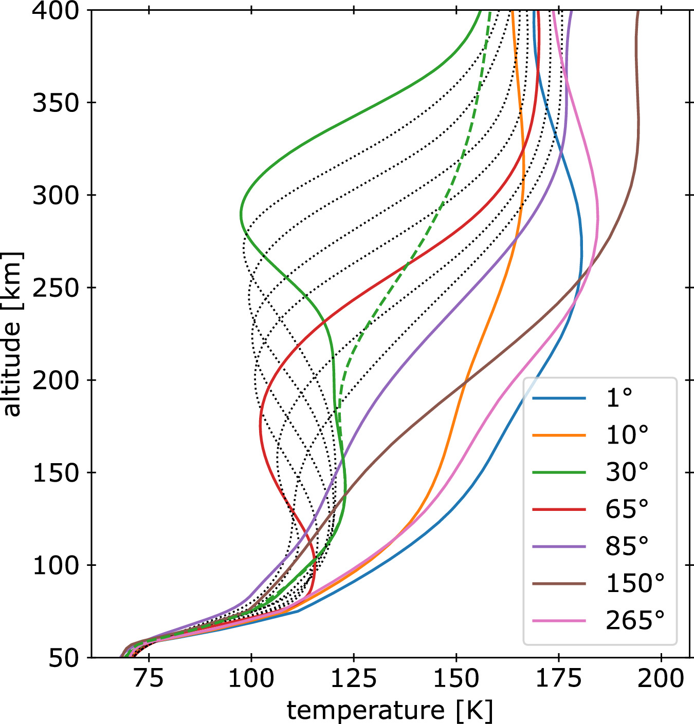
Figure 2. Polar temperature profiles throughout a Titan year for ΔT = 50 K. The dotted lines represent intermediate temperature profiles constructed as described in the text, and the dashed line represents the unmodified Ls = 30° profile (ΔT = 0 K).
Download figure:
Standard image High-resolution image5.2. Reference Simulation
The evolution of atmospheric and cloud variables for this simulation is shown in Figure 3, and profiles from select times are in Figure 4. A layer of lower-stratosphere HCN cloud persists throughout the year around 100 km (see Figure 3 at Ls = 15° and 0°), which is consistent with prior measurements (e.g., Samuelson et al. 2007; Anderson & Samuelson 2011) and microphysical modeling (Lavvas et al. 2011; Barth 2017). HCN first condenses just below 300 km at Ls = 221, where the temperature reaches 120 K, but the cloud remains relatively thin until about Ls = 26°, when temperatures drop below 110 K and the supersaturation grows large enough to efficiently nucleate HCN ice (see Figures 3(c), (f), and (g) and the Ls = 24° and 30° lines in Figure 4).

Figure 3. Atmosphere and cloud variables from Ls = 124 to 925 of the 16th Titan year of the simulation: (a) temperature, (b) HCN vapor mixing ratio, (c) HCN particle number mixing ratio, (d) HCN mass mixing ratio, (e) effective radius of HCN cloud particles, (f) extinction of HCN cloud at 0.889 µm, and (g) HCN supersaturation. The thick black dashed line indicates the descending 110 K isotherm, and the thick black dotted line shows the minimum temperature altitude. Vertical black dotted lines indicate Ls = 24°, 30°, 36°, 45°, and 65°. Other contours are indicated in the figure legends.
Download figure:
Standard image High-resolution image
Figure 4. Profile plots of (a) temperature, (b) vapor volume mixing ratio, (c) number mixing ratio, (d) mass mixing ratio, (e) effective radius, (f) extinction at 0.889 µm, and (g) supersaturation from the same simulation as Figure 3 at Ls = 24°, 30°, 36°, 45°, 65°, and 90°.
Download figure:
Standard image High-resolution imageInitial cloud formation is marked by nucleation of a small number of particles that grow rapidly, resulting in effective radii greater than 10 μm. These particles soon fall out of the cold layer, encounter warmer temperatures, and rapidly sublimate, effectively transporting vapor to lower altitudes (see vapor mixing ratio, qmr, in Figure 4) and leaving the cloud separated or "detached" from the lower-stratospheric cloud by a 150 km deep layer of low extinction (see Figures 3(f) and 4). A similar low-extinction layer appears in imagery from both VIMS (de Kok et al. 2014, their Figure 2; from 2012 June, Ls = 34°) and ISS (West et al. 2016, their Figures 2 and 5(b); with images from 2012 June and 2013 April, Ls = 44°). While the timing of the low-extinction layer in the simulation does not match the observations, these results demonstrate that a cold layer in the upper stratosphere can produce detached cloud consistent with observations. The cloud remains detached until about Ls = 26°, when the stratosphere below 200 km becomes saturated. Once the below-cloud temperature drops beneath the freezing point, cloud particles no longer sublimate but instead fall all the way to the troposphere. Since there is abundant vapor below the cloud, the first particles to reach lower altitudes grow very large, with effective radii >20 μm by the time these particles reach the troposphere (see reff at Ls = 30° in Figure 4). This population of particles produces a local maximum extinction near 150 km at about Ls = 30°, or about 2.5 yr into the simulation (see Figure 3, panel (c) for Nmr and panel (e) for extinction). When stratospheric cooling ceases at Ls = 30°, there is less excess vapor available, and particle sizes at the tropopause steadily decrease.
The temperature minimum near 300 km and Ls = 30° produces a second population of particles nucleated primarily between 300 and about 330 km, where the temperature drops below 120 K. This nucleation event produces many more particles than the initial nucleation, but the increased competition for vapor results in the particles remaining small, with effective radii of <3 μm (Figures 3(d) and 4). These particles fall more slowly, producing the extinction maximum just above 200 km after Ls = 30° (Figures 3(e) and 4). Particles continue to nucleate near 120 K as the low-temperature region descends, but the effective radii stay below 5 μm throughout the upper half of the cloud's depth. Although the temperature below the cloud top continues to decrease, the remaining vapor is insufficient to produce large particles after the initial population precipitates into the troposphere. The simulated 0.889 μm optical thickness of the cloud peaks at about 0.15 at Ls = 30° (the maximum optical thickness at 2.7 μm is about 0.17 at the same time). This is between the estimates by de Kok et al. (2014) and West et al. (2016; see Table 1), which differ by a factor of 100.
The HCN column mass (see Figure 5) increases during the beginning of the year until cloud formation, reaching a maximum of 1.27 g m−2 about 1 Earth yr into the simulation, or Ls = 12°, and shortly after, the temperature begins decreasing throughout the stratosphere (see Figure 2). Cloud condensation and subsequent precipitation result in the rapid removal of HCN from the stratosphere, illustrated in Figure 5, which culminates in the minimum total HCN column mass of 0.225 g m−2, less than a quarter of the maximum, at about 5.7 Earth yr, or Ls = 67°. Nearly half of the annual precipitation out of the stratosphere occurs during the initial cooling period between Ls = 10° and 30°, as the precipitation rate decreases once the stratosphere begins to warm. The HCN column minimum occurs just after the cold layer begins to rapidly warm (Ls = 65° profile in Figure 2). By the winter solstice (Ls = 90°, 7.8 Earth yr), the cold layer becomes indistinguishable from the steep temperature inversion in the lower stratosphere, and HCN condensation is restricted to altitudes at or below 120 km, though the optical thickness of HCN remains >10−2 until nearly Ls = 130° (not shown). This is consistent with earlier observations by Samuelson et al. (2007), who found HCN cloud below 160 km during north polar winter (2005 March 31, equivalent to Ls = 123° in the southern hemisphere). Furthermore, Mathé et al. (2020, their Figure 12) find that HCN vapor above 200 km is depleted in early northern winter but gradually replenishes between 2005 (Ls = 301°) and 2011 (Ls = 28° of the next year), consistent with the simulated total HCN vapor column (Figure 5). In summary, the HCN column increases until cloud formation begins in early fall, at which point precipitation rapidly removes the majority of the HCN. Precipitation effectively ceases by about Ls = 65°, and by Ls = 90°, the HCN cloud is restricted to the lower stratosphere, allowing HCN vapor at higher altitudes to replenish throughout the rest of the year.

Figure 5. Column-integrated mass of stratosphere HCN vapor (solid orange), HCN condensate (solid blue), total HCN (dashed green), and cumulative HCN condensate flux (dotted red) just above the tropopause (51 km). Gray lines and labels on the right mark (from bottom to top) the minimum HCN vapor column, minimum HCN column, maximum condensed HCN column, and net HCN precipitation at 51 km over 1 Titan yr. Vertical black dotted lines indicate Ls = 24°, 30°, 36°, 45°, and 65°.
Download figure:
Standard image High-resolution image5.3. Sensitivity Testing
The previous subsection shows that the simulated cloud is consistent with measurements given the following parameters: ΔT = 50 K, f = f0, snuc = 35%, w300 = 0 m s−1, and Kdiff = KT92 (see Table 2). In order to test the sensitivity of the model to changes in these parameters, we ran further simulations using different combinations of these additional values: ΔT = 40 or 30 K, f = 0.1 × f0 or 10 × f0, snuc = 5%, w300 = −2 or −0.2 mm s−1, and Kdiff = 5 × KT92 or 0.2 × KT92 (all simulations relevant to this publication are tabulated in Table 3). All simulations were run for 4 or more Titan yr, and we use the last year for analysis. These additional simulations show that the primary conclusions from Section 5.2 are insensitive to these parameters; the cloud always forms by Ls = 30° and descends, following the cold layer, until it reaches the lower stratosphere around Ls = 60°, and precipitation always removes over half of the total column mass of HCN during the fall season. The output for the f = 0.1 × f0 simulation is shown in Figures 6 and 7 as an example. Versions of Figures 3, 4, and 5 for each simulation are archived along with the simulation output in the Johns Hopkins data repository.
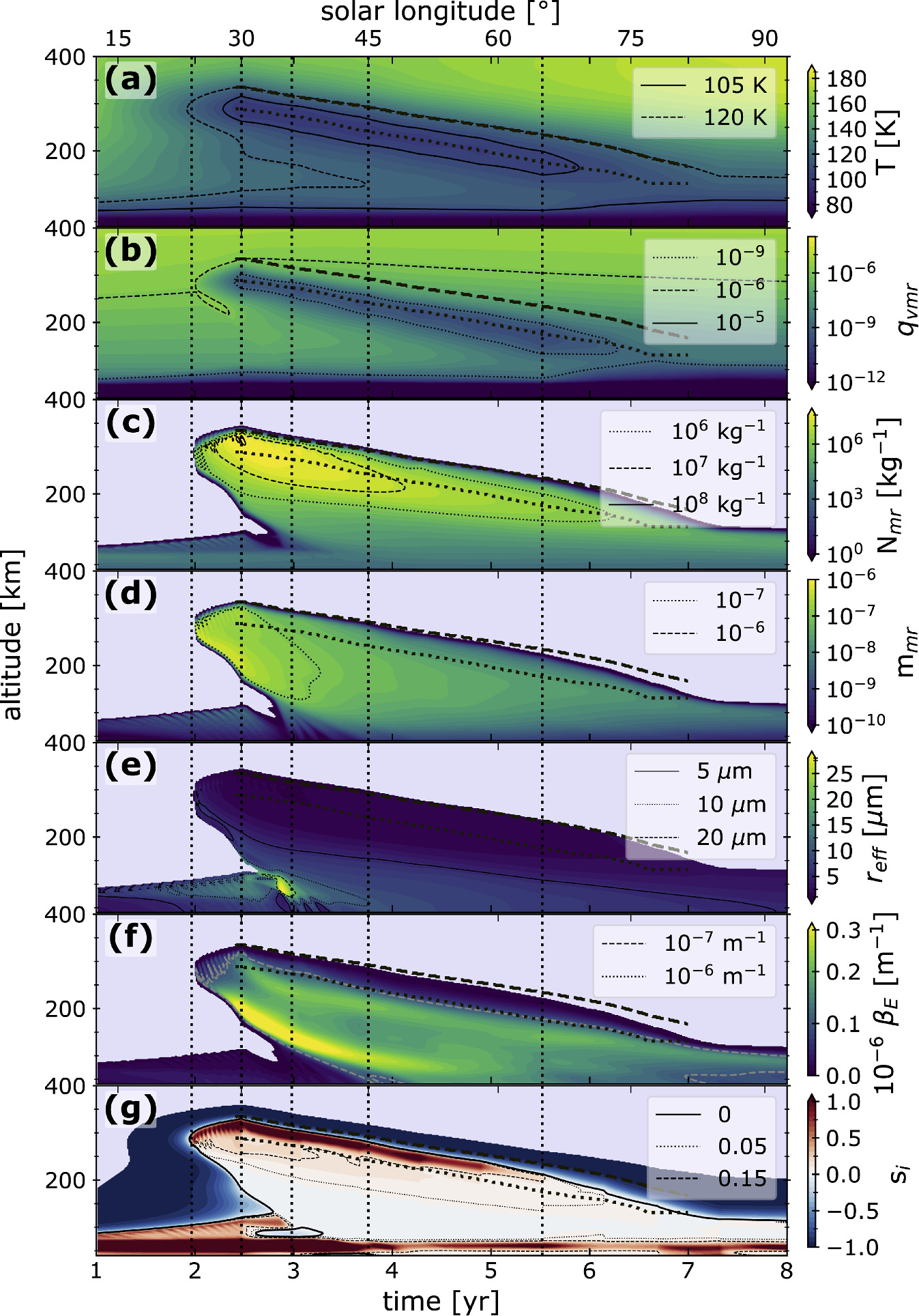
Figure 6. Same as Figure 3 but for f = 0.1 × f0.
Download figure:
Standard image High-resolution image
Figure 7. Same as Figure 4 but for f = 0.1 × f0.
Download figure:
Standard image High-resolution imageTable 3. Consistency of Simulation Output with Observations
| 0.1 × f0 | f0 | f0, snuc = 5% | f = 10 × f0 | |
|---|---|---|---|---|
| ΔT = 30 K | ↓Nmr, ↓q400, ↓τv | ↓Nmr, ↑reff | ↓Nmr | ↑reff, ↓Nmr, ↑q400 |
| ΔT = 40 K | ↓q400 | ✓ | ✓ | ↑reff, ↓Nmr, ↑q400 |
| ΔT = 50 K | ↓q400 | ✓ | ↑Nmr | ↑q400 |
| ΔT = 30 K, w300 = −2 mm s−1 | — | — | — | ⋯ |
| ΔT = 40 K, w300 = −2 mm s−1 | — | — | — | ⋯ |
| ΔT = 50 K, w300 = −2 mm s−1 | ↑q400, ↓τv | ↑q400, ↓τv | ↑Nmr, ↑q400, ↓τv | ⋯ |
| ΔT = 30 K, w300 = −0.2 mm s−1 | ↓Nmr, ↓τv | ↓Nmr, ↑q400 | ↓Nmr, ↑q400 | ⋯ |
| ΔT = 40 K, w300 = −0.2 mm s−1 | ↓q400 | ↑q400 | ↑q400 | ⋯ |
| ΔT = 50 K, w300 = −0.2 mm s−1 | ↓q400 | ↑q400 | ↑Nmr, ↑q400 | ⋯ |
| ΔT = 50 K, Kdiff = 5 × KT92 | ↑Nmr, ↓q400 | ↑Nmr, ↓q400 | ↑Nmr, ↓q400 | ↑Nmr |
| ΔT = 50 K, Kdiff = 0.2 × KT92 | ↓Nmr | ↓Nmr, ↑q400 | ↓Nmr, ↑q400 | ⋯ |
Download table as: ASCIITypeset image
5.3.1. Cold Layer Temperature
Larger ΔT consistently produces cloud with smaller reff, larger Nmr, larger τv , lower vapor abundance at 400 km, and earlier nucleation with a longer detached period. ΔT = 30 K simulations result in reff = 5 μm, while for ΔT = 50 K simulations, reff = 1–2 μm.
5.3.2. Vapor Flux
The rate and timing of the maximum precipitation intensity, the duration of the detached period, and the vertical optical thickness all depend on the vapor flux (see Figure 8(b)). Lower f corresponds with a delay in the peak precipitation from 2.3 Earth yr (Ls = 28°; see Figure 8) to 3–4 Earth yr (Ls = 36°–48°), while with f = 10 × f0, the peak precipitation occurs earlier, between 1.7 and 2 Earth yr (Ls = 21°–24°). Similarly, lower f causes delayed cloud formation and extends the detached period from less than half an Earth year (see Figure 3(f)) to close to a full Earth year (Figure 6(f)), though with smaller vertical optical thickness.

Figure 8. (Upper) HCN precipitation flux at 51 km and (lower) cumulative 51 km HCN precipitation. Colors indicate ΔT, where blue is ΔT = 50 K, orange is ΔT = 40 K, and green is ΔT = 30 K. Line style indicates the flux and nucleation supersaturation, where solid is f = f0, dashed is f = 0.1 × f0, dashed–dotted is f = 10 × f0, and dotted is f = f0 with snuc = 5%. Vertical black dotted lines indicate Ls = 24°, 30°, 36°, 45°, and 65°.
Download figure:
Standard image High-resolution image
5.3.3. Nucleation Efficiency
Increasing the nucleation efficiency by setting snuc = 5% decreases the cloud particle effective radius and increases the optical thickness and net precipitation mass. The effects of snuc on the vapor mixing ratio at 400 km are insignificant.
5.3.4. Subsidence
Weak subsidence of w300 = −0.2 mm s−1 (this vertical velocity is from Teanby et al. 2006 for 60°N during northern winter; similarly, Achterberg et al. 2008 estimate a vertical wind speed of w300 = −0.5 mm s−1 at 60°N during winter and summer, and de Kok et al. 2008 estimate w300 = −0.15 mm s−1 for polar northern winter) results in enhanced vapor at 400 km but has only small effects on the other observed variables.
5.3.5. Eddy Diffusivity
The most significant effect of adjusting Kdiff is changing the rate of vapor transport from the top of the model. The sedimentation timescale for cloud particles is significantly shorter than the diffusion timescale, so the impact on cloud particle transport is minimal. Because they affect the vapor transport, changes to subsidence, w300, and eddy diffusivity, Kdiff, both affect the slope of the vapor abundance with respect to altitude, which governs the supply of vapor to the cloud. Increasing Kdiff consistently increases Nmr and decreases q400, while decreasing Kdiff has the opposite effect on both variables.
5.3.6. Comparison with Observations
Only a subset of the tested scenarios result in cloud that is consistent with observations. Table 3 catalogs the simulations in addition to how they compare with observed values of Nmr, reff (as listed in Table 1), τv using the condition 10−2 ≤ τv ≤ 2, and q400 using the condition 10−5 ≤ q400 < 10−4 (see Section 2.2 for discussion of the validation conditions). Actual values of reff, Nmr, τv , and q400 for each simulation scenario are tabulated in the Appendix in Tables A1 and A2. Check marks indicate that the 6 month mean and the instantaneous values at 300 km and Ls = 30° are both consistent with all four observed quantities, arrows indicate that the simulated value was higher (up arrow) or lower (down arrow) than the observed value, dashes indicate that no cloud formed, and ellipses indicate that the scenario was not modeled. Overall, we find that 300 km temperatures of T300 = 97–107 K (ΔT = 40 and 50 K) are consistent with observations, and this conclusion is relatively insensitive to changes in simulation parameters. The remainder of this section focuses on how our simulations compare with reported values of each quantity.
The simulated cloud particle number mixing ratio, Nmr, was too low for all of the warmest simulations, where ΔT = 30 K, which is consistent with the findings from Section 3.2. Simulations with efficient nucleation, snuc = 5%, at ΔT = 50 K have Nmr in excess of observed values except when vapor transport is impeded by decreasing the eddy diffusivity, Kdiff. Efficient nucleation can increase the minimum temperature required to match the observed Nmr, but the effect is not significant enough to make simulations with ΔT = 30 K compatible with the observations.
Effective radii, reff, were always within the observed range except when ΔT = 30 K with nominal vapor flux. In this case, the few particles that nucleated reached large enough sizes to grow efficiently and deplete the vapor even at relatively low supersaturations.
None of the simulations produced a 0.889 μm vertical optical thickness consistent with West et al. (2016), who estimated 0.6 ≤ τv < 2; the largest simulated vertical optical thickness is about 0.3 when ΔT = 50 K and f = 10 × f0 (see the Appendix for all τv values), but this scenario was not considered, as it has unrealistically large HCN mixing ratios. Because the τv estimates by de Kok et al. (2014) and West et al. (2016) differ, we use the entire range of both τv estimates to evaluate the simulations in Table 3. The modeled τv falls between the two estimates, 0.07 < τv < 0.6, for every scenario with efficient nucleation, snuc = 5%, and nearly every scenario with ΔT = 50 K, except in the presence of a strong downdraft, w300 = −2 mm s−1. In general, lower temperatures, increased vapor flux, efficient nucleation, and subsidence are all associated with larger cloud optical thickness. Changes to Kdiff have inconsistent effects on τv .
HCN vapor abundance at 400 km is below the reference value of 10−6 in scenarios with reduced vapor flux, f = 0.1 × f0, though this can be offset by subsidence or decreasing the eddy diffusivity to Kdiff = 0.2 × KT92. Increasing the eddy diffusivity to Kdiff = 5 × KT92 produces a similar result as reducing the vapor flux. However, as discussed in Section 2.2, Mathé et al. (2020) reports lower HCN vapor mixing ratios of ∼10−6. Six scenarios produced q400 ∼ 10−6, but since four of these six scenarios are disqualified by multiple variables, relaxing the q400 condition to 10−6 < q400 < 10−4 based on retrievals from Mathé et al. (2020) admits only the ΔT = 40 and 50 K scenarios with decreased vapor flux as consistent with observations.
In summary, sensitivity testing indicates that cloud formation consistent with observations requires 300 km temperatures of approximately T300 = 97–107 K. Simulations over this temperature range remain consistent with observations when the vapor flux is decreased if we introduce weak subsidence. In the case of enhanced nucleation efficiency, only the upper end of the temperature range remains within the range of the observed variables. This conclusion is consistent with the results outlined in Section 3.2, and it is insensitive to uncertainties in other model parameters.
6. Concluding Remarks
6.1. Conclusions
As predicted by de Kok et al. (2014), we find that the formation of the 300 km south polar cloud requires temperatures far colder than contemporaneous measurements and that these conditions result in the majority of the vapor being rapidly removed from the stratosphere. We model the observed cloud by introducing a cold layer at 300 km, which then descends to the lower stratosphere. Although HCN condensation begins at higher temperatures, the observed cloud particle number mixing ratio, effective radius, and optical depth only occur at temperatures around T300 = 97–107 K, which is 40–50 K lower than the minimum temperature observed at 300 km and about 15 K lower than the temperature estimated by de Kok et al. (2014). Using synthetic temperature profiles, measurements by Teanby et al. (2019), and temperature profiles retrieved by Vinatier et al. (2020) at 86°S and Ls = 658, we model the descent of a cold layer from its initiation at Ls = 30° until it reaches the cold lower stratosphere at Ls = 85°. The cloud is initially detached from the lower stratosphere by a deep low-extinction layer, where particles sublimate as they precipitate out of the supersaturated region. This low-extinction layer persists for a few Earth months before stratospheric cooling halts the sublimation of precipitating particles. Once precipitation from the cloud reaches the condensation in the lower stratosphere (Ls = 30° in Figures 3 and 4 and Ls = 36° in Figures 6 and 7), we find that precipitation from the ∼300 km deep cloud results in the rapid removal of the majority of the HCN in the stratosphere (see same times in Figures 5 and 8). By the winter solstice, HCN condensates exist only in the lower stratosphere, and HCN vapor is already being replenished throughout the rest of the stratosphere.
These conclusions are largely insensitive to changes in most model parameters. More efficient HCN nucleation (snuc = 5%) results in cloud formation at higher 300 km temperatures, though only the T300 = 107 K (ΔT = 40 K) case is consistent with observations, as T300 = 97 K (ΔT = 50 K) produces too many particles, and T300 = 115 K (ΔT = 30 K) produces too few particles. Finally, weak downward motion of w300 = −0.2 mm s−1 can be offset with decreased HCN flux (f = 0.1 × f0) for simulations to remain consistent with observations if we relax the lower constraint on the 400 km HCN vapor abundance, q400. Thus, we conclude that our primary results are robust to the significant uncertainties in the temperature profile and microphysical properties of HCN and Titan's haze.
6.2. Discussion
The rapid precipitation that we see in mid-fall may lead to HCN on the surface being concentrated in polar regions while also seeding tropospheric methane and ethane clouds and potentially enhancing precipitation that could contribute to the lakes and seas found in Titan's polar regions. Smaller HCN particles with slower fall speeds are less likely to serve as ice nuclei and may circulate throughout the troposphere before they reach the surface. Precipitation from clouds in the upper stratosphere expedites the transport of HCN vapor from the upper atmosphere to the surface and may prevent its circulation and condensation throughout the rest of the stratosphere. Although we focused on HCN, it is possible that other volatile species could be similarly affected by precipitation, which complicates the use of volatiles as tracers during polar winter. A scarcity of polar CIRS observations between 2012 and 2017 limits our understanding of how the abundances of these gases evolve throughout the season, but observations just before the end of the Cassini mission in 2017 reveal dramatic decreases in the stratospheric abundances of several volatile species (Coustenis et al. 2020; Vinatier et al. 2020). Precipitation may explain better than chemical lifetime or circulation patterns why the stratospheric HCN concentration increases less than concentrations of other trace gases during polar fall (see, e.g., Teanby et al. 2019; Sharkey et al. 2021, their Figures 4(n) and 15, respectively). Since concentration gradients in volatiles such as HCN and HC3N are frequently used to infer atmospheric circulation patterns (e.g., Teanby et al. 2019; Coustenis et al. 2020; Vinatier et al. 2020), a better understanding of precipitation in polar winter is critical for understanding polar vortex dynamics.
Several areas deserve further study, including observational verification of the simulated cloud evolution, model and laboratory studies of the impact of simultaneous condensation of multiple species, and cloud microphysical simulations that include other atmospheric processes like radiation and convection. While Le Mouélic et al. (2018) catalog several VIMS multispectral images of the cloudy south polar region during southern fall and show HCN ice signatures, no radiative transfer analysis of these images revealing macro- or microphysical cloud properties has been published to date. Analysis of these VIMS data between 2014 and 2017 could reveal the optical thickness, cloud-top altitude, and microphysical properties of the HCN cloud and potentially other condensates. Additional details regarding the evolution of the cloud in south polar fall are necessary to better understand the impact of the cloud on the radiative and volatile budgets, as well as the polar circulation. In addition to HCN, there is evidence of condensed C6H6, HC3N, and C4N2, as well as ice composed of multiple co-condensed compounds, in polar fall and winter clouds (Coustenis et al. 1999; Anderson & Samuelson 2011; Anderson et al. 2014, 2018a, 2018b; Vinatier et al. 2018). Stratospheric microphysical cloud models up to now have only included the condensation of individual volatile species (Barth 2017; Dubois et al. 2021), entirely neglecting potential interspecies interactions. Future modeling work should explore the implications of simultaneous condensation of multiple species, as well as co-condensation as mixed crystals. Finally, despite evidence of significant radiative cooling (e.g., Teanby et al. 2017) and convective motions (West et al. 2013, 2016), the present work excludes cloud radiative, convective, and dynamic interactions. Integration of condensation into dynamical models, including Titan global circulation models, will be critical for understanding the role of clouds and condensation in Titan's polar stratosphere.
Acknowledgments
We would like to thank the two anonymous reviewers for their input, as well as the editorial staff and administrative staff at our institutions that made our work and this publication possible. L.E.H. and D.W. acknowledge support from NASA FINESST grant 80NSSC21K1760 and Solar System Workings grant 80NSSC20K0138. E.B. acknowledges support from Cassini Data Analysis Program grant 80NSSC20K0485. C.M.A. acknowledges partial funding from the NASA Planetary Science Division Internal Scientist Funding Program through the Fundamental Laboratory Research (FLaRe) work package, as well as NASA's Cassini Data Analysis Program.
Software: xarray (Hoyer & Hamman 2017), Matplotlib (Hunter 2007).
Data Availability
Model output and plots of the simulations discussed in this paper are archived in the Johns Hopkins data repository at 10.7281/T1/UZIT7C.
Appendix: Simulation Output Values
For each simulation scenario, we compare both the instance and 6 month mean values at Ls = 30° of Nmr, reff, τv , and q400 to the observed values provided in Table 1. The results of this comparison are shown in Table 3, instantaneous values of each of these variables are listed in Table A1, and 6 month mean values are listed in Table A2. Dashes indicate cloud did not form in a given simulation and ellipses indicate the scenario was not simulated.
Table A1. Instantaneous Effective Radius, Particle Number Mixing Ratio, Optical Thickness, and HCN Abundance at Ls = 30°
| Value | f = 0.1 × f0 | f0 | fo, snuc = 5% | f = 10 × f0 | |
|---|---|---|---|---|---|
| ΔT = 30 K | reff | 4.8 | 6.8 | 4.0 | 13.6 |
| Nmr | 1.1 × 10³ | 9.8 × 10⁴ | 5.5 × 10⁶ | 3.0 × 10⁵ | |
| τv | 4.2 × 10⁻³ | 4.2 × 10⁻² | 1.0 × 10⁻¹ | 6.4 × 10⁻² | |
| q400 | 5.1 × 10⁻⁶ | 4.8 × 10⁻⁵ | 5.0 × 10⁻⁵ | 5.0 × 10⁻⁴ | |
| ΔT = 40 K | reff | 1.2 | 2.9 | 2.1 | 6.8 |
| Nmr | 5.4 × 10⁷ | 1.5 × 10⁷ | 1.3 × 10⁸ | 4.8 × 10⁶ | |
| τv | 2.0 × 10⁻² | 9.4 × 10⁻² | 1.7 × 10⁻¹ | 1.8 × 10⁻¹ | |
| q400 | 5.4 × 10⁻⁶ | 5.0 × 10⁻⁵ | 5.0 × 10⁻⁵ | 4.8 × 10⁻⁴ | |
| ΔT = 50 K | reff | 1.1 | 2.0 | 1.7 | 4.0 |
| Nmr | 7.7 × 10⁷ | 6.7 × 10⁷ | 1.3 × 10⁸ | 3.1 × 10⁷ | |
| τv | 2.8 × 10⁻² | 1.5 × 10⁻¹ | 2.1 × 10⁻¹ | 3.0 × 10⁻¹ | |
| q400 | 5.0 × 10⁻⁶ | 4.8 × 10⁻⁵ | 4.8 × 10⁻⁵ | 4.6 × 10⁻⁴ | |
| reff | — | — | — | ⋯ | |
| ΔT = 30 K, | Nmr | — | — | — | ⋯ |
| w300 = −2 mm s−1 | τv | 2.4 × 10⁻³ | 2.2 × 10⁻⁴ | 1.8 × 10⁻⁴ | ⋯ |
| q400 | 6.4 × 10⁻⁵ | 4.1 × 10⁻³ | 4.1 × 10⁻³ | ⋯ | |
| reff | — | — | — | ⋯ | |
| ΔT = 40 K, | Nmr | — | — | — | ⋯ |
| w300 = −2 mm s−1 | τv | 1.8 × 10⁻⁴ | 2.1 × 10⁻⁴ | 1.9 × 10⁻⁴ | ⋯ |
| q400 | 4.1 × 10⁻⁴ | 4.0 × 10⁻³ | 4.0 × 10⁻³ | ⋯ | |
| reff | 0.6 | 0.6 | 0.6 | ⋯ | |
| ΔT = 50 K, | Nmr | 2.3 × 10⁷ | 3.8 × 10⁷ | 2.3 × 10⁸ | ⋯ |
| w300 = −2 mm s−1 | τv | 6.9 × 10⁻⁴ | 1.7 × 10⁻³ | 1.0 × 10⁻² | ⋯ |
| q400 | 1.8 × 10⁻³ | 4.0 × 10⁻³ | 1.8 × 10⁻² | ⋯ | |
| reff | 2.4 | 7.4 | 3.3 | ⋯ | |
| ΔT = 30 K, | Nmr | 9.0 × 10⁴ | 1.1 × 10⁵ | 9.3 × 10⁶ | ⋯ |
| w300 = −0.2 mm s−1 | τv | 5.3 × 10⁻³ | 4.3 × 10⁻² | 1.1 × 10⁻¹ | ⋯ |
| q400 | 1.3 × 10⁻⁵ | 1.3 × 10⁻⁴ | 1.3 × 10⁻⁴ | ⋯ | |
| reff | 1.7 | 3.1 | 2.3 | ⋯ | |
| ΔT = 40 K, | Nmr | 1.9 × 10⁷ | 1.4 × 10⁷ | 4.8 × 10⁷ | ⋯ |
| w300 = −0.2 mm s−1 | τv | 2.2 × 10⁻² | 1.0 × 10⁻¹ | 1.8 × 10⁻¹ | ⋯ |
| q400 | 1.3 × 10⁻⁵ | 1.3 × 10⁻⁴ | 1.3 × 10⁻⁴ | ⋯ | |
| reff | 1.2 | 2.2 | 1.9 | ⋯ | |
| ΔT = 50 K, | Nmr | 7.2 × 10⁷ | 6.3 × 10⁷ | 1.2 × 10⁸ | ⋯ |
| w300 = −0.2 mm s−1 | τv | 3.4 × 10⁻² | 1.6 × 10⁻¹ | 2.2 × 10⁻¹ | ⋯ |
| q400 | 1.3 × 10⁻⁵ | 1.2 × 10⁻⁴ | 1.2 × 10⁻⁴ | ⋯ | |
| reff | 0.6 | 1.1 | 0.7 | 2.5 | |
| ΔT = 50 K, | Nmr | 4.6 × 10⁸ | 4.0 × 10⁸ | 1.8 × 10⁹ | 1.5 × 10⁸ |
| Kdiff = 5 × KT92 | τv | 2.2 × 10⁻² | 1.5 × 10⁻¹ | 1.3 × 10⁻¹ | 3.2 × 10⁻¹ |
| q400 | 9.4 × 10⁻⁷ | 8.1 × 10⁻⁶ | 8.2 × 10⁻⁶ | 7.0 × 10⁻⁵ | |
| reff | 2.1 | 4.8 | 3.5 | ⋯ | |
| ΔT = 50 K, | Nmr | 1.1 × 10⁷ | 3.1 × 10⁶ | 1.1 × 10⁷ | ⋯ |
| Kdiff = 0.2 × KT92 | τv | 3.1 × 10⁻² | 9.4 × 10⁻² | 1.9 × 10⁻¹ | ⋯ |
| q400 | 2.2 × 10⁻⁵ | 2.1 × 10⁻⁴ | 2.1 × 10⁻⁴ | ⋯ | |
Note. Italics indicate that the value is consistent with de Kok et al. (2014) for τv (0.01–0.07) or Mathé et al. (2020) for q400 (10−7–10−6).
Download table as: ASCIITypeset image
Table A2. 6 Month Mean Effective Radius, Particle Number Mixing Ratio, Optical Thickness, and HCN Abundance at Ls = 30°
| Value | f = 0.1 × f0 | f0 | fo, snuc = 5% | f = 10 × f0 | |
|---|---|---|---|---|---|
| ΔT = 30 K | reff | 4.0 | 6.3 | 4.0 | 14.7 |
| Nmr | 2.8 × 10² | 2.4 × 10⁵ | 2.7 × 10⁶ | 2.5 × 10⁵ | |
| τv | 2.8 × 10⁻³ | 3.3 × 10⁻² | 8.5 × 10⁻² | 5.4 × 10⁻² | |
| q400 | 5.1 × 10⁻⁶ | 4.8 × 10⁻⁵ | 5.0 × 10⁻⁵ | 5.0 × 10⁻⁴ | |
| ΔT = 40 K | reff | 1.6 | 3.3 | 2.5 | 7.4 |
| Nmr | 1.6 × 10⁷ | 1.0 × 10⁷ | 3.7 × 10⁷ | 3.1 × 10⁶ | |
| τv | 1.6 × 10⁻² | 8.3 × 10⁻² | 1.5 × 10⁻¹ | 1.6 × 10⁻¹ | |
| q400 | 5.4 × 10⁻⁶ | 5.0 × 10⁻⁵ | 5.0 × 10⁻⁵ | 4.8 × 10⁻⁴ | |
| ΔT = 50 K | reff | 1.3 | 2.2 | 1.7 | 4.5 |
| Nmr | 5.0 × 10⁷ | 4.6 × 10⁷ | 1.1 × 10⁸ | 2.2 × 10⁷ | |
| τv | 2.4 × 10⁻² | 1.4 × 10⁻¹ | 1.9 × 10⁻¹ | 2.7 × 10⁻¹ | |
| q400 | 5.0 × 10⁻⁶ | 4.8 × 10⁻⁵ | 4.8 × 10⁻⁵ | 4.6 × 10⁻⁴ | |
| reff | — | — | — | ⋯ | |
| ΔT = 30 K, | Nmr | — | — | — | ⋯ |
| w300 = −2 mm s−1 | τv | 2.3 × 10⁻³ | 2.2 × 10⁻⁴ | 1.8 × 10⁻⁴ | ⋯ |
| q400 | 6.4 × 10⁻⁵ | 4.1 × 10⁻³ | 4.1 × 10⁻³ | ⋯ | |
| reff | — | — | — | ⋯ | |
| ΔT = 40 K, | Nmr | — | — | — | ⋯ |
| w300 = −2 mm s−1 | τv | 1.8 × 10⁻⁴ | 2.1 × 10⁻⁴ | 1.9 × 10⁻⁴ | ⋯ |
| q400 | 4.1 × 10⁻⁴ | 4.0 × 10⁻³ | 4.0 × 10⁻³ | ⋯ | |
| reff | 0.6 | 0.7 | 0.6 | ⋯ | |
| ΔT = 50 K, | Nmr | 1.5 × 10⁷ | 2.4 × 10⁷ | 1.8 × 10⁸ | ⋯ |
| w300 = −2 mm s−1 | τv | 4.2 × 10⁻⁴ | 1.2 × 10⁻³ | 7.8 × 10⁻³ | ⋯ |
| q400 | 1.8 × 10⁻³ | 4.0 × 10⁻³ | 1.8 × 10⁻² | ⋯ | |
| reff | 3.3 | 7.0 | 4.0 | ⋯ | |
| ΔT = 30 K, | Nmr | 1.8 × 10⁴ | 1.1 × 10⁵ | 9.3 × 10⁶ | ⋯ |
| w300 = −0.2 mm s−1 | τv | 3.6 × 10⁻³ | 3.6 × 10⁻² | 9.4 × 10⁻² | ⋯ |
| q400 | 1.3 × 10⁻⁵ | 1.3 × 10⁻⁴ | 1.3 × 10⁻⁴ | ⋯ | |
| reff | 2.0 | 3.5 | 2.7 | ⋯ | |
| ΔT = 40 K, | Nmr | 1.1 × 10⁷ | 9.6 × 10⁶ | 3.1 × 10⁷ | ⋯ |
| w300 = −0.2 mm s−1 | τv | 1.7 × 10⁻² | 9.1 × 10⁻² | 1.6 × 10⁻¹ | ⋯ |
| q400 | 1.3 × 10⁻⁵ | 1.3 × 10⁻⁴ | 1.3 × 10⁻⁴ | ⋯ | |
| reff | 1.4 | 2.4 | 1.9 | ⋯ | |
| ΔT = 50 K, | Nmr | 5.2 × 10⁷ | 4.6 × 10⁷ | 1.1 × 10⁸ | ⋯ |
| w300 = −0.2 mm s−1 | τv | 2.7 × 10⁻² | 1.5 × 10⁻¹ | 2.0 × 10⁻¹ | ⋯ |
| q400 | 1.3 × 10⁻⁵ | 1.2 × 10⁻⁴ | 1.2 × 10⁻⁴ | ⋯ | |
| reff | 0.8 | 1.4 | 0.8 | 2.8 | |
| ΔT = 50 K, | Nmr | 2.7 × 10⁸ | 2.4 × 10⁸ | 1.3 × 10⁹ | 1.1 × 10⁸ |
| Kdiff = 5 × KT92 | τv | 1.9 × 10⁻² | 1.3 × 10⁻¹ | 1.2 × 10⁻¹ | 3.0 × 10⁻¹ |
| q400 | 9.4 × 10⁻⁷ | 8.1 × 10⁻⁶ | 8.2 × 10⁻⁶ | 7.0 × 10⁻⁵ | |
| reff | 2.2 | 4.9 | 3.4 | ⋯ | |
| ΔT = 50 K, | Nmr | 5.7 × 10⁶ | 1.6 × 10⁶ | 7.2 × 10⁶ | ⋯ |
| Kdiff = 0.2 × KT92 | τv | 2.5 × 10⁻² | 8.3 × 10⁻² | 1.7 × 10⁻¹ | ⋯ |
| q400 | 2.2 × 10⁻⁵ | 2.1 × 10⁻⁴ | 2.1 × 10⁻⁴ | ⋯ | |
Note. Italics indicate that the value is consistent with de Kok et al. (2014) for τv (0.01–0.07) or Mathé et al. (2020) for q400 (10−7–10−6).
Download table as: ASCIITypeset image