


Abstract
The quest to find extraterrestrial life is a critical scientific endeavor with civilization-level implications. Icy moons in our solar system are promising targets for exploration because their liquid oceans make them potential habitats for microscopic life. However, the lack of a precise definition of life poses a fundamental challenge to formulating detection strategies. To increase the chances of unambiguous detection, a suite of complementary instruments must sample multiple independent biosignatures (e.g., composition, motility/behavior, and visible structure). Such an instrument suite could generate 10,000× more raw data than is possible to transmit from distant ocean worlds like Enceladus or Europa. To address this bandwidth limitation, Onboard Science Instrument Autonomy (OSIA) is an emerging discipline of flight systems capable of evaluating, summarizing, and prioritizing observational instrument data to maximize science return. We describe two OSIA implementations developed as part of the Ocean World Life Surveyor (OWLS) prototype instrument suite at the Jet Propulsion Laboratory. The first identifies life-like motion in digital holographic microscopy videos, and the second identifies cellular structure and composition via innate and dye-induced fluorescence. Flight-like requirements and computational constraints were used to lower barriers to infusion, similar to those available on the Mars helicopter, "Ingenuity." We evaluated the OSIA's performance using simulated and laboratory data and conducted a live field test at the hypersaline Mono Lake planetary analog site. Our study demonstrates the potential of OSIA for enabling biosignature detection and provides insights and lessons learned for future mission concepts aimed at exploring the outer solar system.
Export citation and abstract BibTeX RIS

Original content from this work may be used under the terms of the Creative Commons Attribution 4.0 licence. Any further distribution of this work must maintain attribution to the author(s) and the title of the work, journal citation and DOI.
1. Introduction
1.1. The Search for Life
The search for life beyond Earth is a driving theme in the 2022 Planetary Science Decadal Survey (National Academies of Sciences, Engineering, and Medicine 2023) to address the civilization-level question, "Are we alone?" To translate this search into well-defined planetary mission concepts, we draw insight from our current understanding of terrestrial life while accepting the fewest assumptions possible to preserve sensitivity to exotic forms. On Earth, all life requires access to water. Our solar system includes several bodies known or suspected to contain liquid water, including the icy moons of Jupiter and Saturn with their ancient, deep internal oceans (Hendrix et al. 2019). Some of these "ocean worlds" feature plumes of liquid water streaming into space (Hansen et al. 2011), forming natural sampling opportunities for life detection missions. Even Mars, with its comparatively dry environment, may contain lava tubes with subsurface aquifers sufficient to support past or current microbial communities (Léveillé & Datta 2010). While the complexity, size scale, and biochemistry of potential extant life are exceedingly difficult to predict, terrestrial environments suggest that our search should begin with simple, microscopic forms. Bacteria and archaea are the most ubiquitous and numerous forms of life on Earth, significantly predating all multicellular life and surviving in the widest variety of habitats (Donoghue & Antcliffe 2010) including analog environments similar to what may lie within Enceladus and Europa (Marion et al. 2003; Hand et al. 2017). Therefore, recent mission concepts have focused on instruments to detect microscopic life in aqueous environments.
1.2. Instruments for the Search
Life detection is a uniquely challenging scientific objective for two reasons. First, there remains considerable disagreement on the fundamental definition of life on Earth (Lovelock 1965). Second, for any single proposed biosignature, there are abiotic processes that can generate similar, misleading signals. This is exacerbated on other planetary bodies where dominant physical processes may substantially differ from those studied on Earth (Steele et al. 2022). To address this, life detection missions should include the capability to detect conceptually orthogonal biosignatures that together reduce the likelihood of misinterpretation of biotic and abiotic phenomena.
The Europa lander mission concept introduces a "biosignature bingo" template, where multiple biosignature results can be combined to aid in the joint assessment of a given site (Hand et al. 2017, 2022). Proposed instruments to inform this process include a surface stereo camera, luminescence microscope, Raman spectrometer, and gas chromatograph-mass spectrometer among others. Similarly, the Enceladus Orbilander mission concept by MacKenzie et al. (2021) identifies independent science objectives to be satisfied by a high-resolution mass spectrometer, laser-induced fluorescence, a separate separation-capable mass spectrometer, and an optical microscope. Finally, the OWLS instrument suite includes six instruments, including three microscopes, a mass spectrometer, an organic molecules detector, and laser-induced fluorescence (Lindensmith et al. 2022). Many of these proposed instruments are modeled after those found in modern biological laboratories and can generate gigabytes of data per observation. While such data volumes are routinely accommodated in a laboratory setting, the need for space missions to communicate all findings across vast interplanetary distances and through over-subscribed resources like the Deep Space Network makes communication bandwidth a primary bottleneck for planetary exploration. Put simply, the compelling detection of extraterrestrial life may require over 10,000 times more raw data than is transmissible by a space mission.
1.3. Data Bandwidth Limitations at Interplanetary Distances
The physical limitations of data transmission for planetary missions—known as the "bandwidth barrier"—directly hinders the search for extant life (Castano et al. 2007; Theiling et al. 2022) and was identified as a major challenge in the recent Planetary Science Decadal Survey (National Academies of Sciences, Engineering, and Medicine 2023). This limitation results primarily from the inverse square law that governs electromagnetic propagation. The recent mission concepts for the Enceladus Orbilander and Europa Lander estimated downlink transmission rates of 34 kbit s−1 and 48 kbit s−1, respectively (MacKenzie et al. 2021; Hand et al. 2022). This is less than the 56 kbit s−1 achievable with dial-up internet and would require roughly an hour to transmit a single, uncompressed 12 megapixel image from a modern phone camera. At the same time, life detection mission concepts are pushing the boundaries on large data volume instruments. For just one of the microscopic imagers in the OWLS instrument suite, a one minute observation generates as much data as the entire Enceladus Orbilander's surface mission data budget (MacKenzie et al. 2021) and approximately 40 times that of Europa Lander (Hand et al. 2017). Beyond the physical data rate limitation, all deep space missions must also rely on the already over-committed Deep Space Network, further limiting communications opportunities and returned data volume (Hackett et al. 2018). While technology upgrades such as optical communication are underway, these are anticipated to result in at most a 40× improvement (Deutsch 2020). Therefore, novel mission strategies are required to accommodate high data volume instruments in the planetary context.
Missions currently accommodate the bandwidth barrier by limiting the number of observations, but this approach is poorly suited to the search for life. In this strategy of "take only what raw data can be returned," no observations are requested beyond the available downlink or other limitations (e.g., available power, thermal management, onboard data storage, and competing instrument schedules). For example, the Orbilander concept proposes making up to seven observations with most life detection instruments during the 176 day primary science phase. This would total ∼1 GB of raw data when including the large data volume nanopore sequencer (or ∼0.29 GB without it; MacKenzie et al. 2021). This strategy, in the context of traceable science requirements and budget minimization, often drives mission design: why engineer a spacecraft capable of capturing more data than can be returned? While this prioritizes efficient usage of scarce planetary exploration funding, it can also hinder statistically robust sampling of a remote environment and any associated science conclusions. In the MRO/HiRISE example, observations covering only 3%–4% of the surface of Mars were returned between 2006 and 2022, leaving most of the planet unexplored at higher resolution (McEwen et al. 2010; Mcewen et al. 2022). In the case of life detection, this strategy is distinctly problematic for two reasons. First, compelling biosignatures may be relatively rare in collected observations. Second, for every observation containing a strong biosignature, many more will be required to statistically characterize that signal, contextualize it against a heterogeneous background, explore and falsify abiotic interpretations, and inform a process-level understanding of its origin. Low sample numbers incur the catastrophic risk that exotic life is encountered but not captured in instrument observations or that a lone detection cannot be defensibly substantiated (Levin & Straat 2016).
The second method currently used by missions to address limited downlink bandwidth is through data compression techniques, but these cannot produce the compression factors needed without heavy scientific cost. General purpose data compression methods (such as JPEG, MP3, and MP4) and specialized methods for mission operations such as ICER (Kiely & Klimesh 2003) offer tunable, lossy compression of at most 10×–50× with minimal apparent degradation. For some space applications such as hazard cameras, landing footage, and contextual panoramas, these techniques are useful means to reduce downlink strain. However, while all of these methods were designed to minimize the perception of degradation, they still introduce compression artifacts that can distort and obscure scientific conclusions, limiting their safe application to very low compression ratios (Kerner et al. 2018). Likewise, while generic, lossless compression algorithms also exist that remove redundancy, such as PKZIP, they do not result in significant gains when applied to raw science observations. To achieve the four-orders-of-magnitude reduction needed to enable high-volume instruments while preserving valid scientific conclusions, generic compression algorithms will play a limited role. Instead, we require a solution that is driven by a mission's specific science goals and ensures that the most scientifically informative evidence is returned to Earth.
1.4. Managing the Bandwidth Barrier with OSIA
OSIA is a unique subfield of the broader autonomy pursuit focused on science observation content analysis and empowering mission science teams. OSIA seeks to maximize a mission's scientific return in the presence of harsh bandwidth constraints relative to instrument data volumes, limited communications opportunities, rare or transient observations of interest, or unanticipated environments. It comprises two broad onboard capabilities: observation summarization and data prioritization. Summarization encompasses the capabilities to recognize, characterize, and extract meaningful information from raw observational data. Summarization algorithms must support as similar scientific conclusions as possible while also reducing the data volume of raw observations by several orders of magnitude. Prioritization provides an ordering of summarized or raw observations based on their contents' scientific relevance and contextual importance to the current mission. It can function both within a single instrument's observational record, as well as in the larger context between multiple instruments. A given mission concept may benefit purely from summarization when raw observation contents can be well modeled and efficiently extracted, purely from prioritization when rare but recognizable signals are of primary concern, or from their joint application in more complex situations. In all cases, OSIA cannot and should not claim to reach scientific conclusions or advance science itself, but rather remain focused on accelerating and extending the mission science team's understanding and control over observation acquisition and downlink.
1.5. OSIA in the Broader Autonomy Context
OSIA is complementary to, but distinct from, several system-level autonomy applications such as proximity operations (Nesnas et al. 2021), onboard cruise navigation (Bhaskaran 2012), onboard planning and scheduling (Gaines et al. 2022), and automated surface mobility (Rankin et al. 2020). While OSIA systems are innately focused on recognizing content within science observations, they can provide alerts and guidance to onboard planning and scheduling systems to trigger follow-on observations or inform observation site selection. Similarly, OSIA can be used to monitor traditionally engineering-focused inputs like hazard avoidance cameras during auto-drive sequences to assess sites of potential scientific interest, to build a record of imagery content, as well as justify decisions to halt for potential hazards or priority science targets. To minimize impact on other flight systems, OSIA may be bundled with a dedicated computer and storage within a "smart instrument" package.
Prior to the OWLS project, several OSIA implementations were demonstrated on late-phase missions with the purpose of building traceable heritage. These early systems tended to be single-purpose and intentionally simple in construction to help overcome perceived risk and present clear value propositions such as biosignature-related mineralogy detection (Mandrake et al. 2012) and opportunistic, transient phenomenon capture (Castano et al. 2008). The most mature OSIA example yet produced is the Autonomous Exploration for Gathering Increased Science (AEGIS) system for Mars rovers, operationally deployed on both Curiosity and Perseverance (Francis et al. 2015, 2017). By enabling autonomous target acquisition for the ChemCam and SuperCam instruments, AEGIS provides a systematic baseline site characterization during periods when the rover would otherwise be idle and has increased mission science yield for ChemCam from 256 to 327 collections per sol (Francis et al. 2017). In each case, these examples were opportunistically deployed within architectures not originally intended for onboard analysis. Earlier inclusion of OSIA during the mission formulation process (as in OWLS) would enable new missions and scientific objectives, rather than acting as ad hoc enhancements to existing systems.
1.6. OSIA Driving Requirements
OSIA adoption faces challenges due to its operational position between scientists and their raw observations (McGovern & Wagstaff 2011). Figure 1 visualizes this unique Concept of Operations (ConOps) strategy. To engender trust with mission stakeholders, we propose that OSIA be subject to several novel requirements (Slingerland et al. 2022). (1) To increase transparency and verification, a summary of data products should include multiple, overlapping extractions from each observation that make different assumptions and use unrelated algorithmic approaches. (2) To support future advances in modeling and analysis, summary products should be accompanied by select, supporting raw data. (3) Observation prioritization should consider explicit science targets of interest, the relative diversity between observations, and the data that has already been returned to the ground. (4) Whether adapting to an evolving science mission focus or changing instrument characteristics, OSIA must provide sufficient information about its treatment of observation contents to allow mission operations to recognize the need for and enable OSIA reconfiguration. (5) OSIA must return sufficient insight to inform manual observation downlink requests, and honor those requests at the highest priority when they occur. (6) Extracted parameters of interest from observations should be accompanied by an estimate of uncertainty to both inform interpretation and capture potential mismatch between the onboard models and observation contents.
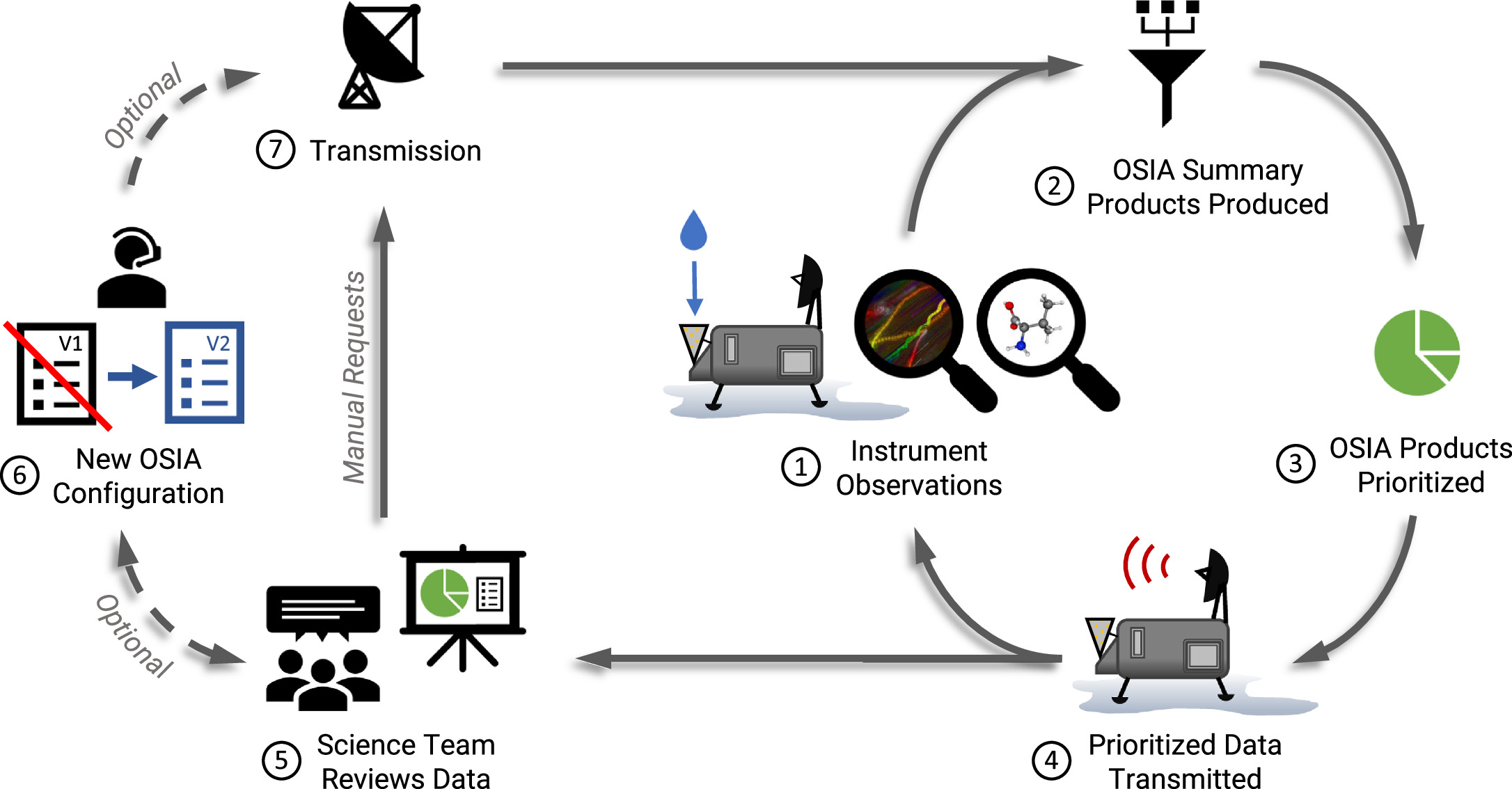
Figure 1. OSIA collects, analyzes, summarizes, and prioritizes scientific observations collaboratively with science team guidance and reconfiguration. This simplified illustration depicts a general OSIA ConOps strategy. Step 1: Ocean world lander collects surface samples and acquires instrument observations. Step 2: OSIA assesses and summarizes instrument data according to its current configuration and manual ground requests. Step 3: OSIA prioritizes available data products by estimated science value and, optionally, with respect to what has already been returned. Step 4: The highest-priority science data products are transmitted to Earth, maximizing downlink capacity. Lower-priority data is retained onboard for potential downlink at a later point in time. Step 5: Ground science teams review new observations vs. outstanding science questions and determine whether the OSIA's behavior requires redirection. Step 6: If so, scientists and operators generate an updated configuration that is most responsive to the current science intent. Step 7: Any manual data requests and new configurations are transmitted.
Download figure:
Standard image High-resolution imageIn the following Sections, we will specifically consider the OWLS instrument suite, evaluate its need for OSIA treatment, formulate requirements to drive system design, articulate the chosen implementation, and validate its performance on simulated, laboratory, and field observations.
2. The Ocean Worlds Life Surveyor
To empower the search for microbial life on distant planetary bodies, the Jet Propulsion Laboratory has developed the OWLS. OWLS is a mature, Technology Readiness Level (TRL) 5, suite of six integrated instruments and onboard software designed to capture and recognize a range of chemical and biological biosignatures in liquid water samples (Lindensmith et al. 2022). Three microscopes focus on cellular-scale, biological biosignatures within the same sample volume of water: a Digital Holographic Microscope (DHM) to capture video of self-propelled motility at 185 nm scales, a co-observing Fluorescence Light-Field Microscope (FLFM) to capture video of compounds related to cellular walls, proteins, and nucleic acids at 230 nm scales, and a separate High Resolution Fluorescent Imager (HRFI) that captures complimentary still imagery similar to the FLFM at 60 nm scales (Bedrossian et al. 2017; Serabyn et al. 2019; Kim et al. 2020). OWLS also includes three capillary electrophoresis instruments focused on molecular-scale, chemical biosignatures: an ElectroSpray Ionization Mass Spectrometer (ESI-MS) detects biomolecules such as amino acids, the Laser Induced Fluorescence (LIF) instrument analyzes the distribution of chirality in amino acids, and the Capacitively Coupled Contactless Conductivity Detection (C4D) detects organic molecules important to terrestrial metabolism such as tricarboxylic acid and phosphate (Jaramillo et al. 2021; Oborny et al. 2021; Mora et al. 2022; Willis et al. 2022).
The current OWLS instrument suite is embodied as an integrated, field-tested engineering prototype designed to evaluate current life detection technology and inform upcoming mission opportunities. During operation, an observation begins as an aqueous sample is delivered to a preparation system that filters out constituents larger than 40–50 μm and adjusts the sample's salinity and particle concentration by increasing or decreasing water content. The prepared sample is then divided between two paths: one is passed directly to the microscopes for biological investigation (as described in the following Sections) while the second is treated with heat and pressure to rupture any cellular structures and enable chemical investigation.
2.1. Instrument Data Volumes
As shown in Table 1, three of the OWLS instruments produce observations with sufficient data volume as to benefit from OSIA treatment for planetary applications. In this work, we describe OSIA developed for the DHM and FLFM with the associated available software 4 (Wronkiewicz et al. 2023). The third instrument, the ESI-MS mass spectrometer to detect small molecules indicative of life, has an equivalent OSIA software package called Autonomous CE-ESI Mass-spectra Examination (ACME), previously described in Mauceri et al. (2022).
Table 1. Typical Raw and Lossless Compressed Data Volumes for a Single Observation from Each OWLS Instrument
| Instrument | Observation Type | Typical Observation | Lossless Compressed |
|---|---|---|---|
| Size (MB) | (ZIP) Size (MB) | ||
| FLFM | Video (3D: 2D + time) | 1,258 | 523 |
| DHM | Video (3D: 2D + time) | 1,258 | 1,095 |
| ESI-MS | Ion Count Image (2D) | 100 | 71 |
| HRFI | Image (2D) | 21 | 16 |
| C4D | Time Series (1D) | 9 | 5 |
| LIF | Time Series (1D) | 1 | 1 |
| Total | 2,647 | 1,711 | |
Download table as: ASCIITypeset image
The DHM was included on OWLS for its ability to image cell-sized particles in a relatively deep sample chamber (using interferometry) permitting an assessment of 3D motion. A sample is drawn smoothly through the chamber at 5 μL min−1 during imaging, continually exposing new particles to inspection. By capturing holographic images at 15 frames s−1, the DHM enables the disambiguation of self-propelled particle motility from Brownian motion and fluid dynamics (Wallace et al. 2015). Motility is a compelling biosignature that describes the purposeful movement of an organism, such as to search for nutrients, respond to stimuli, or avoid predators (Nadeau et al. 2016). Likely because of its impact on the fitness of a species, motility mechanisms have evolved independently in numerous terrestrial organisms (Miyata et al. 2020). In the extraterrestrial context, this biosignature is also fully chemistry- and composition-agnostic. The top row of Figure 2 shows example DHM frames through time containing a motile microorganism, and the top of Figure 3 shows a close-up of this same microorganism. We implemented an OSIA package—Holographic Examination for Lifelike Motility (HELM)—to track particle movement within raw DHM observations and estimate the probability that a given particle exhibits motility. HELM's purpose is to identify and characterize evidence of lifelike motion and ensure that data containing these biosignatures is prioritized for transmission to ground teams for further assessment.

Figure 2. DHM (top row) and FLFM (bottom row) microscopes simultaneously collect images at 15 frames s−1 permitting detailed analysis of particle motility- and fluorescence-based biosignatures. These example images show the same motile and fluorescent microorganism in 4 s of raw data for both instruments. The microorganism (circled in red) makes a short rightward movement from T = 1 s to T = 2 s and a much longer burst or movement from T = 3 s to T = 4 s. All other particles slowly drift to the right with the background water flow. The observed Moire pattern in the top row is an artifact resulting from the raw holographic encoding, while the gridded appearance of the organism in the bottom row is an artifact of the light field encoding. Note that both microscopes were still in development when this data was taken, resulting in an alignment offset between the two image series.
Download figure:
Standard image High-resolution image
Figure 3. Examples of the same microorganism as it appears in the DHM (top) and FLFM (bottom) microscopes. The images here are particle crops from T = 2 s in Figure 2. Particles in the raw DHM images appear as an Airy pattern that increase in size as the particles become more distant from the central focal plane. Particles in the FLFM appear as a grid of bright spots corresponding to the lenselet array placed in front of the detector. Similarly, the pattern increases in size as the particle is farther from the focal plane. While particles may appear distorted to the naked eye, these images contain volumetric information permitting post hoc refocusing to any focal plane of interest.
Download figure:
Standard image High-resolution imageThe FLFM instrument was included on OWLS to capture particle fluorescence induced by an excitation laser and observes the same sampling volume as the DHM. Fluorescence signals of biological interest can originate from innate chemical structures (e.g., chlorophyll) or through fluorescent tags introduced into a liquid sample that selectively bind to specific molecular structures (e.g., lipids in cell membranes and nucleotides; Nadeau et al. 2008; Serabyn et al. 2019). Both forms of fluorescence permit the measurement of chemical structures known to be important to cellular life on Earth. The bottom row of Figure 2 shows example FLFM frames through time containing fluorescent microorganisms, and the bottom of Figure 3 shows a close-up of a single autofluorescent microorganism. We implemented a second OSIA package—FLFM Autonomous Motility Evaluation (FAME)—to track and characterize fluorescent particles in raw FLFM observations. Due to the common need for particle tracking, FAME shares motility detection algorithms with HELM but includes extensions for fluorescence prioritization. Therefore, FAME has the capability to capture biosignatures related to both cell-like structures as well as motility.
2.2. Reconstruction versus Raw Imagery
The DHM and FLFM both produce raw, 2D images that encode the entire 3D sampling volume through time. This encoding produces considerable visual artifacts and distortion when the raw images are directly examined as shown in Figures 2 and 3. In terrestrial labs with abundant compute resources, mathematical reconstruction methods are repeatedly applied to these raw images, extracting focused images at any specified z-plane above/below the central image plane. These reconstructed images are free of encoding artifacts and form a fully volumetric data set as a function of time. However, image reconstruction is computationally demanding, with full volume reproduction for a single DHM or FLFM observation requiring hours on a modern computer. This is orders of magnitude beyond what is available for flight hardware in the space exploration context. Thus, both HELM and FAME must operate on the raw DHM and FLFM imagery directly, treating volumetric encoding artifacts as a noise source. A natural consequence of this decision is that both systems will be highly sensitive to particles near the central plane of the sample chamber where the raw images are in focus, with steadily reducing sensitivity as particles move away in depth. In practice, this has little direct negative impact on overall sensitivity. If motile or fluorescent particles are present within the chamber, some of them will be near the central image plane long enough to be detected and characterized. Future missions incorporating HELM or FAME could also opt to include a specialized FPGA-based preprocessor to provide reconstructed imagery (Chen et al. 2016) if additional sensitivity to significantly out-of-focus planes is required.
3. Onboard Science Instrument Autonomy for OWLS
3.1. Defining Mission Success: High-level Requirements
Space missions are developed according to hierarchical requirements that extend from high-level, primary science objectives (level 1) to specific performance requirements for each subcomponent (level 4). We defined field test requirements early in the formulation of OWLS to focus on infusion into ocean world missions and lower the barrier for stakeholder trust (Mandrake et al. 2022; Slingerland et al. 2022). Given the novelty of these systems, these requirements may also guide future OSIA-enabled missions on how to articulate and quantify their own needs, following the guidance of Section 1.6. The level 1–3 field test requirements for the OWLS project relevant to its OSIA implementation are shown in Tables A1 and A2, and capture the critical behavior of all OWLS OSIA independent of implementation details. Level 4 field test requirements for HELM and FAME, shown in Table A3, are described later in Section 3.4 with respect to their detailed implementations.
Our requirements and system architecture are driven first by key assumptions on anticipated image contents. (1) Nonsolitarity states that if life is present in a properly prepared, concentrated sample, there should be more than one lone organism to recognize. This is supported both by terrestrial analog sites in Antarctica that contain cells at average concentrations of approximately 7.4 × 10⁴ cells mL−1, as well as the recommended lower limit of microorganism detection for the Europa Lander study of 100 cells mL−1 (Hand et al. 2017). This assumption supports the more attainable onboard goal of recognizing and returning some clear, compelling evidence for life, rather than a stringent requirement for the capture of any and all evidence for life across every observation. A further assumption of Ergodicity states that organisms are expected to freely move through the 3D sample chamber without preference for any particular location. This allows HELM and FAME to directly analyze the raw, unreconstructed observations despite the loss of sensitivity away from the central z-plane as discussed in Section 2.2. An assumption of Uncrowded Observations states that individual organisms will be sufficiently separated within a properly prepared, diluted sample such that their motion track is distinguishable from other particles by a ∼100 pixel distance in the raw microscopy observations. Overly crowded observations containing particles that frequently cross paths are difficult to track and assess for biosignatures. HELM and FAME have been designed to detect and provide warnings when observations violate this assumption. Finally, the assumption of being Well-Resolved states that particles should have sizes between 6 × 6 and 50 × 50 pixels, and their motion should be less than 6 pixels frame−1. The initial sample filtration, sample flow rate, DHM frame rate, and microscope focus may be adjusted to ensure these image-based requirements include sensitivity to the intended microorganisms of interest for a given mission use-case.
3.2. Autonomous Science Data Products and Prioritization Products
A core function of OSIA is its ability to summarize raw observations using a standardized set of autonomous science data products (ASDPs)—distillations of the raw observation containing only the scientifically relevant information. For HELM and FAME, the aforementioned assumptions and requirements (in Tables A2 and A3) drive their design. Specifically, they: (1) must capture scientifically relevant content using orders-of-magnitude less data volume, (2) should each assess the observations from a different point of view and goal, using different algorithms and assumptions, (3) should overlap and be mutually reinforcing, such that one Autonomous Science Data Product (ASDP) may be used to verify others and falsify alternative conclusions, (4) must enable science team analyses and conclusions similar to raw data return, (5) should include strategically selected raw data that substantiate findings and preserve the potential for future data analyses and modeling, (6) must capture sufficient information to detect and respond to the need for OSIA reconfiguration, and finally (7) assess instrument data quality and inform operational monitoring.
Prioritization is realized through the creation of three complementary ASDPs. The first is the science utility estimate (SUE), a positive real number that indicates how similar an observation's contents are to a mission's specified science targets of interest—here, biosignatures indicating life. The SUE produced by HELM corresponds to the evidence of lifelike motility within an observation, while for FAME it must capture both motility and the presence of fluorescence. The second prioritization product is the data quality estimate (DQE), a number that indicates the presence or absence of data quality issues that may impact OSIA function. It provides a mechanism to deprioritize observations that fail one or more data quality checks. The third product is the diversity descriptor (DD), a vector of several scientifically relevant parameters of interest that meaningfully differentiate one observation's contents from another. The DD does not compute a single estimate of "interest" like the SUE; rather, it enables a second mode of prioritization that orders observations by their relative similarity to, or difference from, other observations. The DD could be used to request observations that are "maximally different from what has been already downlinked," "similar to a specific subset of observations," or "best represent the diversity of observations currently onboard." As described later in Section 3.3.6, these three ASDPs enable prioritization (ordering) of observations for downlink. Operationally, HELM and FAME support the dynamic capability to upload new specifications for the SUEs, DQEs, and DDs to reconfigure prioritization as desired by science teams.
3.3. The Autonomy Pipeline
The HELM and FAME data processing pipelines search for biosignatures using a multistep, modular process (Figure 4). Both begin by loading microscope observation image frames, optionally preprocessing them to reduce their resolution, and creating background subtracted versions of the frames. Then, the data validation step assesses the observation's data quality, computes the DQE, and creates some simple contextual ASDPs (Section 3.3.1). After that, particles are identified in individual frames and linked across frames (through time) to form particle tracks (Section 3.3.2). Next, tracks are assessed for biosignatures of interest: HELM identifies signs of motility by extracting track features (Section 3.3.3) and classifying motile movement (Section 3.3.4), and FAME additionally extracts fluorescence characteristics. Finally, ASDPs and prioritization products (i.e., the SUE and DD) are generated for prioritization by Joint Examination for Water-based Extant Life (JEWEL) (Section 3.3.6). Each step is modular and configurable for flexibility during the development cycle and mission operations.

Figure 4. The two OSIA algorithms described in this work (HELM and FAME) were designed as a set of modular components to facilitate iterative development. Each module is configurable to support different or changing use cases.
Download figure:
Standard image High-resolution image3.3.1. Data Preprocessing and Validation
The data preprocessing step applies simple parallelized image manipulations to prepare an observation for further analysis. Both DHM and FLFM data are resized from dimensions of 2048 × 2048 to 1024 × 1024 pixels, which reduces the compute and memory costs of the downstream particle identification and tracking algorithms. The resizing process is parallelizable, and can be configured for even lower resolutions at some cost to particle tracking precision.
The data validation step has two goals: (1) summarize the entire observation to provide contextual information to science teams and (2) execute quality checks to identify potential problems with the instrument or science data. For example, each motion history image (MHI) in Figure 5 provides a quickly interpretable image to understand the quantity and movement characteristics of all particles in an observation. A full list of validation products is described in Table 2. Many products were developed in direct response to science needs or data problems encountered during the development of OWLS. For example, the pixel intensity and pixel difference time series products ensure that observation frames have stable characteristics through time. Large pixel differences between frames can indicate instrument vibration, which will negatively affect particle tracking. The previously described DQE aggregates these pass/fail checks through a weighted summation.

Figure 5. Motion history images (MHIs) compress microscopy observations into a single, quickly interpretable image. Here, color indicates the time when each pixel changed maximally. Left: relatively straight color tracks in DHM (top left) and VFI (bottom left) observations depict particles that passively floated through the sample chamber with the background fluid flow. Right: curving/spiraling tracks in DHM (top right), and reversing tracks in VFI (bottom right) indicate the presence of living, motile cells.
Download figure:
Standard image High-resolution imageTable 2. Data Validation Products Described Here Are Calculated for Both Instruments Unless Specified Otherwise
| Name | Type | Justification |
|---|---|---|
| MHI | Contextual Product | Ground teams need a method to quickly understand observations. This single image summarizes an entire (video) observation by capturing the point in time when the maximum change occurred at each pixel. |
| Median Image | Contextual Product | Single image containing the median value at each pixel location through an entire observation. Used for background subtraction. |
| Pixel Intensity | Bounded Range Check | The mean pixel intensity of frames should lie within an expected range. Values outside this range could indicate incorrect laser configuration or a blockage in sample flow. |
| Pixel Difference | Bounded Range Check | The mean frame-to-frame pixel change should lie within an expected range. Excessive pixel differences could indicate instrument vibration or an over-crowded sample. |
| Estimated Particle Density | Threshold Check | The total number of particles in the field of view should be limited (e.g., through sample dilution) to prevent frequent track crossings (and degradation in tracker performance). |
| Interframe Interval | Distribution Check | The time interval between consecutive observation frames should be consistent. Unsteady frame rates may indicate the acquisition computer is overloaded and will lead to challenges in assessing particle motion. |
| 2D Image Spectrum (DHM Only) | Laser Validation Check | The frequency and power of the three DHM lasers must be properly configured to permit reconstruction. A 2D Fourier spectrum of the observation frames should reflect a known pattern to confirm image reconstruction will be possible by science teams. |
Note. The automated checks are used to calculate the DQE.
Download table as: ASCIITypeset image
3.3.2. Particle Identification and Track Formation
To extract biosignatures, HELM and FAME must first identify and characterize particle motion. Particles are detected in each frame by identifying pixels that are substantially different than the background field (calculated as the median frame across the entire observation). We then apply the DBSCAN algorithm (Ester et al. 1996) to find clusters of pixels meeting a specific size threshold, which are deemed particles. This identification method is agnostic to particle morphology, and tracking directly from the unreconstructed hologram avoids the computationally expensive reconstruction process, which is currently too resource intensive for onboard implementation (Marin et al. 2018).
The particles are then associated into motion "tracks" over time via the linear assignment problem (LAP) tracking algorithm (Jaqaman et al. 2008). The LAP tracker first employs frame-to-frame particle linking, assigning nearby particles in consecutive frames into track segments. This step is spatially global but temporally greedy; it makes no assumptions about particle motion characteristics, but it is also brittle to time gaps in particle detection. Therefore, the tracker employs a second gap-closing step, using global optimization to link the starts and ends of track segments into complete tracks. This method is computationally efficient and produces tracks that are robust to short particle occlusions and overlaps. However, extremely crowded samples can overwhelm the tracker by confusing the initial identification or violating the global assumption—that a particle will be nearest to itself as it moves between frames. If such conditions are expected, increasing the resolution and frame rate can improve the efficacy of this tracking method.
We formalize the particle tracks produced by this step in preparation for the following sections. An observation of n frames of p × p pixel resolution results in a set of tracks K . Each track k ∈ K is a set of particle positions (x, y)t , where x and y are pixel coordinates of the center of the particle, and t is the frame number, representative of time. A track starts and ends at times ts and te , and the particle tracking algorithm imposes a minimum on te − ts to filter out spurious false positive identifications. We formally define a track with Equation (1) as follows:

For all tracks in K , the spatiotemporal coordinates are stored for further biosignature assessment (i.e., motility and fluorescence) in future processing steps. Track coordinates are also included for transmission as the compact collection of integers has a relatively small data volume and permits manual review of particle motion by science teams.
3.3.3. Feature Extraction
Once particles are tracked, HELM and FAME must assess them for signs of motility. To our knowledge, existing systems for motility characterization only evaluate specific species, detect specific patterns (e.g., the run-and-tumble motion of E. coli), or are currently too computationally expensive to deploy on spacecraft-ready computers (Rosser et al. 2013; Son et al. 2015). Instead, we developed an onboard system to identify any motion that cannot be explained by Brownian motion and simple fluid dynamics. The OSIA achieves this by quantitatively describing each track with a feature vector where every element in the vector is calculated using a different movement metric. This vector is then classified by a machine learning (ML) model to estimate the probability of motility.
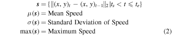
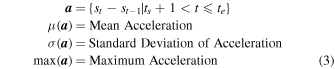
Simple motion features, like speed and acceleration (Equations (2) and (3), respectively), are calculated to identify particles with changing movement patterns. The mean, standard deviation, and maximum value of these discrete values are included as features.
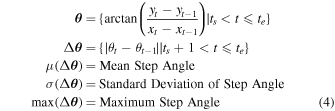
We also measure a particle's step angle at each frame (the discrete angular velocity; Equation (4)), as frequent or large deviations from a straight path suggest motility. Again, the mean, standard deviation, and maximum values are included as features. Here, we omit the conversion of step angle radian values to the range [−π, π] for simplicity.
We can treat each of the speed, acceleration, and step angle features as a time series and measure their autocorrelation for any time lag. This quantifies whether a particle exhibits a movement pattern with some periodicity. We generate features with time lags of 15 and 30 frames (corresponding to 1 and 2 s, respectively), but note that additional time offsets could be added.
In addition to frame-discrete features, we calculate features describing holistic track movement. The length of the track is measured in pixels (Equation (5)) and the duration of the track is measured in frames (Equation (6)). The horizontal, vertical, Euclidean, and angular displacements from the start to end of the track are also measured (Equations (7), (8), (9), and (10); since there is often background fluid flow in the sample chamber, the direction of the total displacement could be indicative of a particle moving against this flow. Sinuosity, the ratio between the track length and the total displacement, quantifies movement inefficiency, as motile particles may appear to meander while exploring for nutrients or responding to stimuli (Equation (11)). Finally, the mean-squared displacement (MSD) slope (as implemented in Manzo & Garcia-Parajo 2015) is used to distinguish Brownian motion from other types of motion.


While these features describe each track independently, we also wish to identify tracks k that behave differently from the set of all other tracks in an observation, { K \k}. We generate the relative speed feature to capture the ratio between a track's mean speed and the mean speed of all other tracks (Equation (13)). Similarly, the relative step angle features are compared between a track's mean step angle and the mean step angle of all other tracks (Equations (16) and (17)). The mean horizontal and vertical displacements of each track (Equations (14) and (15)) are also provided as features.


In total, we compute 23 features to quantify the movement characteristics of each track in preparation for biosignature analysis, but additional features can be added if needed. While these features are not downlinked, they can be recalculated on the ground from downlinked track coordinates. With these track features, HELM and FAME are able to assess tracks for evidence of motility.
3.3.4. Identifying Motility and Fluorescence Biosignatures
After calculating track features, HELM and FAME investigate tracks for evidence of motility and fluorescence. For both, an ML classifier estimates the probability that each track exhibits motile behavior. While the system is agnostic to the ML model used, the computational and interpretability requirements (Table A3) lead us to deploy classical ML methods, including gradient boosted trees (GBTs), random forests (RFs), and support vector classifiers (SVCs). We describe the implementation and evaluation of our model in Section 5.6.2. The posterior probabilities (i.e., confidences) produced by these classifiers further inform data downlink prioritization via the SUE (as discussed in Section 3.3.6). In a flight scenario, the classification model would be trained on the ground and stored onboard for inference with the possibility to retrain and re-transmit new model parameters throughout the mission. FAME also assesses particle fluorescence by directly analyzing the color profile of tracked particles. It calculates maximum particle fluorescence of each color channel and uses this to inform downstream prioritization through both the SUE and DD.
3.3.5. Preparing Downlink Products
Finally, we excise small image crops (or "portraits") from the original, full-resolution DHM or FLFM frames for tracks of interest. These portraits can then be reconstructed on the ground to retrieve a volumetric image of each particle (McKeithen & Wallace 2021) as demonstrated in Section 5.6.3. While these represent important ASDPs as they are portions of the raw data, they also use considerable data bandwidth. Therefore, users can configure the size of particle portraits, the number of desired portraits per track, and optionally limit transmissions to only include portraits for motile tracks in DHM data.
The final output of the OSIA processing pipeline is a list of ASDP bundles from each observation. Each bundle includes: (1) data validation and contextual products, (2) particle tracks and results from their respective biosignature investigations, and (3) original-resolution portraits of scientifically interesting particles.
3.3.6. Prioritizing Autonomous Science Data Products for Downlink
As described in Section 3.2, HELM and FAME compute a SUE, DD, and DQE for each processed observation. HELM's SUE is defined to assign high science importance to observations with tracks that are long in duration and have high motility probabilities. Motile particles that stay in the field of view for a long duration present the best opportunities for further evaluation. First, we score each track by multiplying each track's motility probability, P(motile∣ki ), by its duration, ∣ki ∣. Next, we sum the top five scores, then normalize them to [0, 1] by dividing by the ideal scenario: five full-duration tracks with 1.0 motility probability. This SUE definition is expressed in Equation (18), where k is a track vector as previously defined, n is the duration of the entire observation, and the summation assumes the tracks are sorted by their motility probability. We discuss the efficacy of this SUE definition in Section 5.2.

FAME computes its SUEs by calculating the median of tracks' fluorescence intensities. Since a particle must fluoresce to be observed in FLFM data, the median places scientific value on observations with a population of strongly fluorescing particles.
To quantify diversity, HELM includes particle size, speed, and displacement features in its DD in order to incorporate particle morphology and overall particle movement information into the prioritization. We discuss the efficacy of this definition in differentiating types of observations in Section 5.3.2. FAME defines its DD similarly but also includes the pixel intensities across three image bands to capture the fluorescence profile induced by the binding of different fluorescent tags (or autofluorescence). Refer to Section 3.3.1 for the calculation of the DQE.
To balance utility, diversity, and data quality, a system called JEWEL was developed to prioritize ASDPs from a set of processed observations for downlink (Doran et al. 2021). Intuitively, JEWEL seeks to select ASDPs for observations that balance strong evidence of biosignatures and are also diverse compared to previously transmitted observations' ASDPs. If all instruments calculate the aforementioned prioritization metrics, JEWEL can generate a single prioritization queue for a multi-instrument platform like OWLS. The prioritization algorithm is based on the Maximum Marginal Relevance algorithm (Carbonell & Goldstein 1998), which iteratively selects observations that maximize the additional science utility after applying a "discount factor" based on the most similar observation from those already downlinked. It estimates the similarity of observations by calculating the Gaussian similarity between pairs of DDs (described more in Section 5.3.2) of each candidate observation and the most similar previously downlinked observation. More formally, from the similarity metric, a diversity factor (dfi ) is computed for the ith observation as follows:
where DDj
are the DDs for all previously downlinked data products. The ![$\alpha \in \left[0,1\right]$](https://content.cld.iop.org/journals/2632-3338/5/1/19/revision2/psjad0227ieqn1.gif) parameter provides a mechanism to control the degree to which diversity-based discounting is applied as opposed to using the initial SUE values. When α = 0, the diversity factor is always 1.0 and no discount is applied (e.g., when observations with the strongest identified biosignatures are desired). On the other hand, when α = 1, the similarity-based discount factor is fully applied (e.g., when an equal balance of utility and diversity is desired). After each iteration of selecting a product for downlink, the marginal SUE values are recalculated according to Equation (20) to select the next observation for downlink:
parameter provides a mechanism to control the degree to which diversity-based discounting is applied as opposed to using the initial SUE values. When α = 0, the diversity factor is always 1.0 and no discount is applied (e.g., when observations with the strongest identified biosignatures are desired). On the other hand, when α = 1, the similarity-based discount factor is fully applied (e.g., when an equal balance of utility and diversity is desired). After each iteration of selecting a product for downlink, the marginal SUE values are recalculated according to Equation (20) to select the next observation for downlink:

JEWEL stores a simple onboard manifest of each observation's prioritization metrics and their downlink status to permit future prioritization for an arbitrary number of downlink events.
To engender trust with scientists and mission operators, JEWEL provides two methods of modifying or overriding the OSIA's prioritization decisions. First, JEWEL replicates the commonly used concept of "priority bins" for downlink prioritization, where high-priority ASDPs are transmitted before moving to the next bin. Operators can use a priori knowledge to direct observations ASDPs to specific bins if their importance is known in advance. Mission operators can also use this mechanism to ensure that some nonzero amount of high-priority ASDPs are transmitted for each instrument regardless of the global (across-instrument) prioritization scheme. Second, operators have the ability to manually override SUE values or move ASDPs to different bins during ground-in-the-loop commanding opportunities. This may be necessary, for example, if science teams believe an observation's ASDPs are more (or less) valuable than the OSIA's original estimation. Note that JEWEL also permits different per-bin configurations if a sophisticated prioritization scheme is desired.
While a full operator interface is outside the scope of this work, JEWEL generates an interactive ground report to expose ASDPs and prioritization decisions to ground teams. The visualization displays the cumulative SUE of all downlinked products, a dimensionality-reduced representation of DDs, each observation's DQEs, and a subset of ASDPs. The visualization was developed for the Mono Lake field campaign to quickly inform scientists of any identified biosignatures and explain the OSIA's summarization and prioritization decisions.
3.4. HELM and FAME Field Test Requirements
As discussed in Section 3.1, we defined a set of field test requirements specific to the OSIA described to motivate our work and quantify success at the recently completed OWLS field campaign at Mono Lake, CA. (see the Appendix). While formulating a full mission architecture and the associated flight requirements is beyond the scope of this work, these notional autonomy-focused requirements (Table A3) ensured alignment with the OWLS project scientists and instrument developers. Note that these notional requirements are identical for both HELM and FAME save for extensions related to FAME's additional capability to evaluate fluorescence biosignatures (Req. L4-4). In general, the requirements do not motivate perfect recognition of all biosignatures, but rather ensure that at least one downlink opportunity contains compelling evidence of life. Transmitting false positives has no intrinsic cost, so long as true positives are also returned (Req. L4-1,3). The return of "near miss" examples may also be of scientific interest to provide context for strong evidence of life, and even "clear mistakes" may inform background population studies and potential OSIA improvements or reconfiguration. However, if these false positives crowd out true positives from a downlink opportunity, there is effectively an infinite cost and risk of mission failure (Req. L4-2). Thus, HELM and FAME must quantify the scientific value of any given observation relative to the population of other available observations given the downlink budget (Req. L4-5,6). Beyond prioritizing biosignatures, background and contextual data products are also required to summarize nonprioritized observations in a highly data-efficient manner (Req. L4-8,9). These both inform mission science teams of what might remain onboard and substantiate the high-priority findings. Finally, a computation requirement ensures the timeliness of OSIA in order to support field scientists in real time (Req. L4-7). We present these requirements as demonstrations and to seed discussions with future mission opportunities. The specific, quantified values within each requirement will need updating based on a given mission concept's specific communication budget and risk profile.
4. Data
Data for the development and characterization of OWLS OSIA was assembled from multiple, evolving instrument versions in parallel with the instrument development. Problematic observations were used to develop data validation products as discussed in Section 3.3.1, while high-quality observations were curated into a quantitative evaluation test set. In addition, we developed a DHM data simulator to generate synthetic observations with greater control of instrument and sample properties for sensitivity analyses. Finally, we participated in a field campaign to test the OSIA outside a laboratory setting. Table 3 summarizes these three data sets. For consistency of reporting and evaluation, we standardized all observations to 300 video frames representing 20 s of microscopic footage with an average raw data volume of 1.26 GB. In practice, a mission would be able to dynamically select an observation's frame rate and duration as driven by the current science focus.
Table 3. Summary of Curated DHM and FLFM Data Sets
| Lab | Simulated | Field | ||||
|---|---|---|---|---|---|---|
| DHM | FLFM | DHM | FLFM | DHM | FLFM | |
| Specifications | 2048 × 2048 pixels at 15 frames per second | |||||
| Observations | 41 | 15 | 360 | n/a | ∼137 a | |
| Total Frames | 12,300 | 4,500 | 108,000 | n/a | 241,200 | |
| Total Size (GB) | 50.4 | 18.5 | 433.0 | n/a | 1980.0 | |
| Labeled Tracks | 778 | 199 | 15712 b | n/a | n/a | |
| Labeled Motile Tracks | 213 | 62 | 7815 b | n/a | n/a | |
| Purpose | Quantitative eval. | Sensitivity study | Field eval. | |||
Notes.
a Longer observations split into 300 frame observations. b Labeled by nature of simulation.Download table as: ASCIITypeset image
4.1. Lab Data
The lab data set consists of 41 DHM and 15 FLFM standardized observations of lab-prepared samples. Well-behaved observations without instrument artifacts were chosen in order to quantify our system's performance on realistic data meeting the assumptions described in Section 3.1, representing nominal mission operations. Samples included varying densities of Bacillus subtilis, Chlamydomonas, Euglena gracilis, Shewanella oneidensis, and unknown organisms in water samples returned from the field. For the FLFM, fluorescence was induced in select samples via fluorescent stains (e.g., Syto-9 for nucleic acids or FM1-43 for cell membranes), while in others, autofluorescent organisms (e.g., chlorophyll containing algae) were innately visible. Observations were taken with sample chamber flow rates ranging from 0–5 μL s−1 to evaluate performance over a diversity of sample processing approaches.
To evaluate the performance of the particle tracker and motility classifier (discussed in Sections 3.3.2 and 3.3.4), salient particles were manually tracked throughout each observation and annotated as motile or nonmotile. Labels were generated by external labelers from Labelbox, a data annotation company. To ensure annotation consistency and quality, we provided the labelers with a labeling guide document and video with a specific annotation protocol. All labels were then reviewed for quality by our research team. In total, 778 and 199 tracks were labeled in DHM and FLFM data, respectively. All labeled data including raw observations, labeled tracks, and the labeling guide are published in the JPL Open Repository: doi:10.48577/jpl.2KTVW5 (Wronkiewicz et al. 2022).
4.2. Simulated Data
To further characterize the sensitivity of the particle tracking algorithm, we also generated a simulated DHM data set with a wide range of particle densities, signal-to-noise ratios (S/N), and motility characteristics both satisfying and violating the observation assumptions in Section 3.1. This allowed us to quantify how tracker performance degraded as particles became more crowded and the SNR decreased (see Section 5.6.1). These tracking results also generally apply to the FLFM data, as it uses the same tracking algorithm on an easier task due to the near-zero background fluorescence signal.
DHM observations were simulated by first generating particle tracks, then rendering synthetic particles in individual frames to produce an observation (see Figure 6 for examples). Nonmotile tracks were generated assuming simple Brownian random motion, while motile movement tracks were generated with a Vector AutoRegression (VAR) model fit to labeled tracks from Chlamydomonas observations. A movement bias was then added to both nonmotile and motile tracks to simulate smooth flow in the sample chamber. Each particle was then rendered along the specified tracks as an Airy pattern with a fixed (randomly selected) size and brightness. This resulted in observations with a variety of particle densities and SNRs. With this simulator, 20 observations were generated for each combination of three particle densities and six SNRs, for a total of 360 observations. This simulation procedure can be reproduced using the code and VAR models in our GitHub repository (Wronkiewicz et al. 2023).
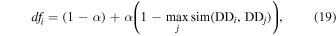
Figure 6. Simulated DHM data for three separate particle densities (from left to right: low, medium, high) and SNR = 2. Increased particle density creates more particle intersections and makes tracking of individual particles more difficult. This figure is available as an animation, which shows the MHIs followed by 20 s of raw simulated data used to generate each MHI.
(An animation of this figure is available.)
Download figure:
Video Standard image High-resolution image4.3. Field Data
The OWLS team conducted a week-long field test of the integrated science instruments, OSIA, and compute hardware at Mono Lake, CA. Mono Lake is a common analog site for ocean worlds, notable for its high salinity as would be anticipated in samples from Enceladus or Europa (Ferreira Santos et al. 2018; Mora et al. 2022). Our team's primary objective was to characterize OSIA performance in a field setting and determine where future development is needed for mission infusion. These results are described in Section 5.1. Our secondary objective was to use the generated ASDPs to assist the science and instrument teams to quickly identify and analyze any biosignatures in collected lake water. Each sampling day consisted of collecting water samples early in the morning from Mono Lake's Station 6 (Humayoun et al. 2003), recording raw data with the six OWLS instruments throughout the day, and applying OSIA to analyze recordings in the evening. While scientists and instrument operators had immediate access to each observations, the sheer volume of data collected meant the OSIA system remained the fastest method to detect biosignatures, identify any instrument issues, and generate a report to facilitate planning for the next day.
At the field side, the particle density of the water samples was extremely high. This led to many particle overlaps within the DHM data. However, the proportion of those particles exhibiting autofluorescence varied widely. Water collected at 5 m contained many autofluorescent particles, while water collected at 35 m was approximately 23 times less dense. Presumably, this difference was due to fewer photosynthetic organisms in the deeper (low-light) conditions. After repeatedly detecting high particle densities for the first three days, the science team prepared a diluted sample on the last day of field work. Unfortunately, an instrument issue prevented that data from being recorded properly. Section 5.1 describes results from the field test in detail.
5. Results
We describe the performance of HELM and FAME with three approaches to substantiate a TRL of 5, as required to participate in mission proposal inclusion. First, we describe our results, takeaways, and lessons learned from evaluating the OSIA during a field test of the integrated OWLS platform at Mono Lake. Second, we quantitatively show that we satisfy the field test requirements described in Section 3.4 by evaluating HELM and FAME on the labeled lab data set described in Section 4.1. Finally, we leverage both our lab and simulated data sets to further characterize the sensitivity of the OSIA system and its submodules.
5.1. Mono Lake Field Test
The OWLS team conducted a week-long field test of the integrated instruments, OSIA, and compute hardware at the Mono Lake, CA. The purpose of this test was to evaluate the OWLS platform at a relevant analog site and expose needed improvements for mission infusion. (See Section 4.3 for details on the data collected.) Below, we describe three key lessons learned from the field test.
First, OSIA expedited scientific discovery especially when biosignatures were rare. Motility, for example, was exceptionally sparse in the recorded DHM data. Only two unambiguously motile organisms were observed, appearing for 12 s in several hours of recorded data (Figure 7). We were able to identify these two motile organisms within about 10 minutes of reviewing the HELM ASDPs at the field site. An abundance of autofluorescent cells was identified in the FLFM data with two examples shown in Figure 8. Mono Lake is known to have high concentrations of Picocystis—a type of green algae—so high concentrations of chlorophyll were expected (Phillips et al. 2021). However, FAME was able to track fluorescent particles and provide a density estimation for the two depths sampled (5 and 35 m), demonstrating requirement L4-4 in Table A3. Overall, the OSIA's ability to rapidly direct attention to the most scientifically relevant data proved valuable in the field setting. For future life detection missions, this same capability could enable an efficient ConOps strategy.

Figure 7. Two motile organisms were captured in MHIs during Mono Lake testing. The left MHI shows a clear zig-zagging movement pattern starting around t = 200. The right MHI shows a cell swimming in a consistently different direction than the passively drifting background particles starting around t = 100.
Download figure:
Standard image High-resolution image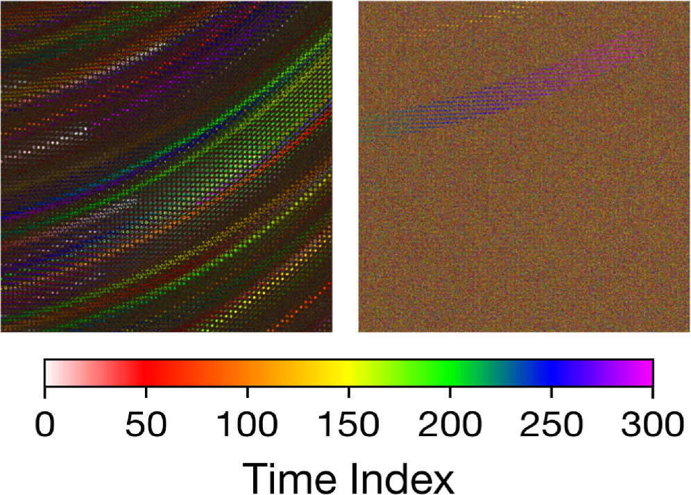
Figure 8. Autofluorescent cells captured at depths of 5 m (left) and 35 m (right) in MHIs at Mono Lake testing. The OSIA detected approximately 23× more autofluorescent particles in the 5 m sample (where light is more abundant). The large majority of fluorescent particles had spectral signatures consistent with chlorophyll. No motile autofluorescent microorganisms were detected at Mono Lake during the field trial.
Download figure:
Standard image High-resolution imageSecond, the data validation and contextual products (see Section 5.4) helped the team efficiently react to the field environment; water samples regularly violated one or more of the data assumptions outlined in Section 3.1. During the first day at Mono Lake, HELM and FAME identified that the water contained particle densities well above the expected range and caused difficulty in tracking particles. Using this insight, the science team planned and carried out sample dilution on Day 4 of the field campaign, demonstrating requirement L3-4 in Table A2. We expect that these automated checks will prove at least as useful in a mission scenario as they did in the field. They could ensure that low-quality data (potentially with incorrect biosignature assessments) does not squander data bandwidth, and that in situ environmental conditions are efficiently communicated to ground teams to inform decisions about instrument operations and OSIA reconfiguration. While reconfiguration of HELM or FAME was not necessary, the capability to do so by editing a plain-text configuration file was available, demonstrating requirement L3-5 in Table A2. Future work on HELM and FAME will explore a wider array of data quality and contextual products to more thoroughly capture real-time data characteristics.
Third, the field campaign reinforced the need for a spectrum of ASDPs ranging from lightly processed summary products (e.g., MHIs) to thoroughly processed, extracted products (e.g., tracks and particle profiles). As mentioned, the Mono Lake field samples contained high particle concentrations well beyond the system's design parameters, simulating a mission instrument miscalibration event. On one hand, FAME performed well under these conditions as only a small fraction of particles possessed strong fluorescent signatures. On the other hand, HELM's tracking performance suffered due to frequent particle crossings, which hindered motility classification. Still, we were able to leverage manual inspection of the MHIs to rapidly identify the two motile organisms present. As future missions will face similarly unpredictable conditions either initially or as instrument performance degrades, an OSIA strategy that incorporates a range of data summarization techniques will be required.
5.2. Observation Summarization
The ability of HELM and FAME to extract scientific content into summary data products with a reduced data volume is their primary means of alleviating bandwidth constraints for missions to ocean worlds. To quantify this capability, we ran both systems on the complete lab-observed data set described in Section 4.1 and computed the ratio of the data volume of raw observations to the "downlink ready" ASDPs. Table 4 summarizes averages over these values.
Table 4. Overview of HELM and FAME ASDPs on the Lab Data Set
| Average Data Volume | ||||
|---|---|---|---|---|
| Autonomous Science Data Products | HELM Configurations | FAME Configurations | ||
| (ASDP) | Low (kB) | High (kB) | Low (kB) | High (kB) |
| Validation Products | 3.7 | 3.7 | 2.4 | 2.4 |
| Motion History Image (MHI) a | 355.4 | 355.4 | 360.6 | 360.6 |
| Particle Tracks | 115.5 | 115.5 | 25.9 | 25.9 |
| Particle Portraits b | 191.8 | 959.0 | 171.0 | 855.0 |
| DD, SUE, DQE | 0.2 | 0.2 | 0.2 | 0.2 |
| Total data volume per sample | 666.6 | 1 433.8 | 560.1 | 1 244.1 |
| Raw Data | 1258393.8 | 1258393.8 | ||
| Lossless Compressed (ZIP) | 1094722.3 | 523100.4 | ||
| Data Reduction (raw/ASDP) | 1887.8 × | 877.7 × | 2246.7 × | 1011.5 × |
| Data Reduction (ZIP/ASDP) | 1642.2 × | 763.5 × | 933.9 × | 420.5 × |
Notes. The low-bandwidth configuration achieves the best data reduction ratio possible, while the high-bandwidth configuration includes more particle portraits. Reported data volumes are averaged over the observed lab data set.
a The resolution of the MHI can be configured to accommodate bandwidth limitations. b Low bandwidth configuration keeps one portrait per track. High bandwidth configuration keeps five portraits per track.Download table as: ASCIITypeset image
Both HELM and FAME are able to produce ASDPs that are 3 orders of magnitude smaller than the original raw data, achieving data reduction ratios of 1887.8 and 2246.7, respectively. These results satisfy the data reduction requirement (Table A2, L3-1). FAME achieves a higher average data reduction ratio because the FLFM only observes fluorescing particles, which are rarer and therefore generate fewer particle track and portrait products. As indicated in Table 4 (Note (a)), the MHI's resolution or lossy compression quality could be increased or decreased depending on the needs of the specific use case. To demonstrate this, the number of particle portraits taken per track was adjusted between the "low-bandwidth" and "high-bandwidth" configurations, as described in Note (b). This allows missions the flexibility to make trade-offs, such as downlinking fewer observations but with more particle portraits per observation.
The choice of summarization configuration is made with respect to each mission's global constraints as well as the science team's current needs. For example, a surface mission on Mars might initially select more and higher-fidelity particle portraits for motile findings, and hence a lower data reduction ratio, given the relatively high bandwidth availability and the initial anticipation that high-priority findings will be rare. However, if a site proved rich in motility signatures, more aggressively compressed results (providing more observations per downlink cycle) might be preferred to quickly understand the diversity of a site. Finally, the science team might choose to return a high-fidelity record of a few select observations of greatest interest, spending their bandwidth to defensibly validate and verify previously summarized findings. This scenario emphasizes the ability to leave raw observations onboard and flexibly reprocess them with differing levels of summarization, responding to an evolving science focus and a growing understanding of the environment both globally and for a local sampling site.
Despite no bandwidth constraint, the terrestrial field trial underscored the need for rapid understanding and focus of attention as would be necessary for planetary use cases. Hundreds of gigabytes of microscopy frames representing hours of observations were recorded each day. As instrument scientists and operators were focused on data collection and occasional hardware debugging, they lacked the time to manually and thoroughly review the entire observational record in real time. Once generated, the ASDPs generated by the OSIA enabled the science team to review each day's full set of observations in 10–20 minutes. After identifying scientifically interesting observations, we could then show the science team the corresponding set of video summaries containing the full OSIA processing results (see Figure 9 for a visualization example). This enabled better planning decisions for the next day's activities and improved the team's understanding of rare events buried within the vast observational record.
Figure 9. HELM and FAME can generate a summary animation of particle motion for science teams to visualize any captured biosignatures. Left: particles are tracked and assessed for motility in a lab data set DHM observation of Chlamydomonas. The animation shows nonmotile and motile particles being tracked and classified (as bright cyan and magenta lines, respectively) as water flows past the field of view. Right: the MHI provides a visual summary of the observation. It is similar to MHIs shown previously except that the pixels corresponding to the current frames max intensity changes are filled in with white. Top: the number of motile and nonmotile particles for the current video frame are displayed to provide context.
(An animation of this figure is available.)
Download figure:
Video Standard image High-resolution image5.3. Observation Prioritization
While high data summarization and reduction rates allow missions to downlink more observations, content-based awareness offers the ability to queue observations for downlink in an order that will best satisfy mission science objectives or accelerate ground teams' understanding of the environment. As described in Section 3.3.6, our OSIA system produces the SUE, DD, and DQE ASDPs to inform JEWEL's prioritization order of data products. To demonstrate prioritization, we apply HELM to the lab DHM data set described in Section 4.1 and prioritize the summarized observations, then analyze the resulting order in terms of successful content recognition.
5.3.1. The Science Utility Estimate
At the start of a mission, science teams seek observations that most directly satisfy the mission's primary science objectives. For HELM and FAME, the SUE, a quantified proxy for the scientific value of an observation, helps identify observations that contain motility or fluorescence biosignatures. JEWEL can be configured to prioritize by simply maximizing the SUE of returned observations. To evaluate the performance of HELM in estimating the SUE, we compare the OSIA-estimated SUEs to the "true" SUEs calculated from human-provided track annotations (Figure 10). As shown, the system demonstrates the generation of skillful SUEs for use during prioritization (per Req. L4-5 in Table A3).

Figure 10. Comparison of OSIA-estimated SUE values to those calculated from ground truth labels on the lab DHM data set. The estimated SUEs exhibit an upward trend with respect to the "true" SUEs calculated from labeled tracks. However, our system slightly overestimates observations with true SUE values <0.2 and moderately underestimates observations with true SUE values >0.4. Three observations are highlighted (triangle, star, diamond) to facilitate deeper discussion into system imperfections and their driving causes.
Download figure:
Standard image High-resolution imageWhile the ideal OSIA system could perfectly estimate SUE values, the most important outcome is that observations are prioritized given the proper relative ordering. Therefore, we compare the sorted lists of observations by their estimated and true SUEs with Kendall's rank correlation coefficient (or Kendall's τ). τ = 1 indicates that the desired and actual ordering match perfectly, whereas τ = 0 indicates no correlation between the orderings. HELM is able to achieve τ = 0.529 on the entire lab data set, rejecting τ = 0 with a p-value of 1.09 × 10⁻⁶. Kendall's τ could be used by future works improving upon this system to benchmark their SUE-based observation prioritization. Additionally, mission concepts could define their OSIA prioritization requirements by determining an acceptable τ for autonomous downlink prioritization through rigorous trade studies.
To explore more deeply the remaining challenges in our system and observations, we investigated three performance cases from Figure 10 to understand how faithfully HELM's SUE calculations represented the data. First, the orange triangle in Figure 10 is a representative observation from a population of low-interest data (true SUE 0–0.2) that is overestimated by 0.1–0.2. In this observation, only one true motile track was found during labeling, which lasted through nearly the entire observation. However, due to a high particle density (exceeding assumptions described in Section 3.1), HELM identified many tracks with 0.4–0.6 motility probabilities. This characterizes the system's response to overcrowding: an overestimation of the utility due to motility. While undesirable, fortunately, this inflation is not sufficient to crowd out legitimately high-interest observations.
Second, the green star is an example where HELM generated an appropriate SUE value. Annotators identified 10 motile tracks, with the top five tracks ranging from 100–250 frames in duration. HELM also identified many of these tracks with similar durations and motility probabilities ranging from 0.6–0.8. Even in these nominal observations, the estimated SUEs tend to be lower than the ground truth, with most samples sitting below the red dashed diagonal of perfect estimation. We attribute this to the ability of human annotators to track motile particles for their entire duration with absolute confidence, while the automated tracker generally captures partial tracks due to confounders, even with existing mechanisms that combine track fragments. Should a mission concept require better SUE accuracy (if abundant high-SUE samples are expected, for example), model calibration (discussed in Section 5.6.2) and general tracker and instrument improvements could address this underestimation. For our use cases, however, the relative prioritization order was minimally affected as all samples' SUEs were consistently underestimated.
Finally, the purple diamond in Figure 10 is a high-interest example where the SUE was underestimated. Annotators identified 10 motile tracks, with the top five tracks lasting all 300 frames. HELM identified its top five tracks with durations ranging around 200 frames, with motility probabilities ranging from 0.4–0.6. However, the particles were at the limits of detection and sometimes overlapped, leading to track fragmentation. The classifier was also less confident with these motility patterns, consisting of slowly curving paths that were not well represented in the rest of the training data. This supports the need to further expose the system to a robust set of motility styles, both real and simulated, once mission resources become available for a full flight implementation.
5.3.2. The Diversity Descriptor
We also include the DD as a component of prioritization to ensure a diverse set of samples comprise the final prioritized list. Whereas the SUE provides a mechanism to exploit an environment by identifying specific biosignatures, the DD provides a mechanism to explore samples across a range of conditions. It enables the autonomy to distinguish between different categories of observations independent of the SUE. On a real mission, diversity-based sampling would be most relevant once the primary science objectives of a mission were met, or if the initial SUE was a poor fit for the spacecraft's environment; in such situations, ground teams might desire a holistic understanding of the target environment's variability both for exploration and to help identify new biosignatures for SUE reformulation.
To define the DD vectors, we identified track metrics that reasonably separated the different observations into similar groups. For HELM, we used a 9D vector using the 10th, 50th, and 90th percentiles of the size, speed, and end-to-end displacement of tracks within each observation. For FAME, we use the same percentiles for fluorescent intensity, acceleration mean, and step angle mean. Therefore, the DD demonstrated the capability to separate lab and natural samples as well as different flow conditions and organism characteristics (per Req. L4-6 in Table A3).
5.3.3. Prioritization Tuning
Figure 11 shows three exemplar approaches to prioritizing DHM observations using different relative weights for the SUE and DD using the prioritization framework outlined in Section 3.3.6. The color of each point indicates an observation's SUE value, while the axes indicate an observation's relative relationship to others using DD elements. For intuitive visualization, we have plotted against only two of the original nine DD elements.

Figure 11. A variety of prioritization strategies are achieved through different weighting of the SUE (indicated by marker color) and the DD (indicated by marker position). These plots indicate the top 10 prioritized observations (in red text) from 41 lab training data sets using three different strategies: scientific utility-only (left), a balance between utility and diversity (middle), and diversity-only (right). The utility-only prioritization selects high-SUE experiments without regard for the DD and chooses several observations judged to contain highly similar in content (as indicated by their proximity in this plot). The middle plot demonstrates a balanced prioritization (with α = 1.0 in Equation (19)) where selected experiments have a higher mean SUE, but also provide a sampling of the DD space. The right plot shows diversity-only prioritization with selections spanning the DD space without regard for the SUE. Note: the true DD vector is 9D, as specified in Section 3.3.6. We artificially chose two of the DD elements here—the 90th percentile of the track particle size and 50th percentile track speed—to visually convey the prioritization concept.
Download figure:
Standard image High-resolution imageA utility-only prioritization scheme (Figure 11, left) ranks observations based solely on the SUE. In our evaluation data, this prioritizes lab observations containing dozens of clear, motile Bacillus subtilis (B.Sub.) organism tracks. The speed and size of tracked particles in these observations was fairly consistent (comprising most of the grouping toward the lower left). Such a scheme is most beneficial when ground teams are confident in both their restricted interest in specific biosignatures and that the OSIA is well tuned to identify these key observations.
In contrast, a diversity-only prioritization scheme (Figure 11, right) ranks observations by the difference from the set of all previously transmitted observations (using the DD hyperspace as a quantitative proxy). After an initial, high-SUE observation is selected, the rest are sequentially chosen by their distance/difference from the previously selected observations. This includes natural samples from Newport Beach, CA on the right side of the plot which had large particles and were relatively fast. A diversity-focused prioritization strategy may be desirable after the primary mission science objectives are achieved or if the initial transmitted observations fail to satisfy a mission's science objectives and contextual information is needed to retune the OSIA. They also can provide key awareness of unexpected observation contents critical to inform instrument and OSIA reconfiguration.
However, a science team will often desire a blend of utility-based and diversity-based prioritization (Figure 11, middle). Here, the lower-left cluster of observations (with many motile organisms) is still sampled, but some observations containing large and/or fast particles (right and top of the plot, respectively) are also included despite lower utility scores. A balanced strategy allows a mission to pursue its stated science objectives while maintaining awareness of unexpected observation content. As the relative weighting between SUE and DD is a tunable parameter (see Equation (19)), ground teams can update the prioritization strategy as their understanding grows. Taken together, these analyses demonstrate that our OSIA system meets the L3-2 requirement for data prioritization, as described in Table A2.
5.4. Data Validation
In addition to science summary products, the data validation step includes simple checks to identify observations that violate expected data characteristics and alert operations teams. If unrecognized, these observations may hamper downstream biosignature analysis. Refer to Section 3.3.1 and Table 2 for the full list of validation products generated by HELM and FAME. Figure 12 illustrates two data quality checks and related observations that violate each. The top panel of Figure 12 shows one observation containing vibration recorded while the DHM was only partially integrated into OWLS. It also includes an observation in which the microscope was physically bumped during recording, causing sharp frame-to-frame shaking. Any microscope movement is important to detect as it can induce fictitious motility-like movement in observed particles. The bottom panel of Figure 12 shows a second problem where observations from the field campaign contained high particle densities. In this situation, particles appear to regularly intersect in the raw 2D observations causing degraded tracker performance. Section 5.6.1 (and Figure 14) provides a more thorough sensitivity analysis of how high particle density can degrade tracking performance. For any observation, failing one or more data quality checks translates to a lower DQE and impacts its assessment during data prioritization. Given similar SUE and DD values, this ensures high-quality observations are favored for downlink. For each check included in the DQE, the acceptable bounds and relative weight compared to other checks are configurable to permit retuning by ground teams. In addition to the DQE, all validation failures are logged to verbose plain text reports for operator review. This capability, demonstrated during the field test described in Section 5.1, satisfies Requirements L4-8,9 in Table A3.

Figure 12. Data validation products help identify quality issues in observations. Here, time traces indicate instrument vibration and shaking (top; red and orange, respectively) as well as excessive particle density in DHM and FLFM observations from the Mono Lake field campaign (bottom; red and orange, respectively). The blue trace and shaded region indicates the (expected) mean and interquartile ranges of these same metrics for the training data. The threshold for each validation check (indicated by the black dotted line) is a tunable parameter that determines if each observation passes or fails. Large frame-to-frame changes and high particle density can both degrade tracking performance and downstream biosignature analysis, so detecting these problems can help influence prioritization and alert ground teams to potential instrument issues.
Download figure:
Standard image High-resolution image5.5. Computational Performance and Flight Software Integration
HELM and FAME were developed to accommodate limited flight computing resources, including efficient algorithms and flexibility for flight hardware architecture such as multiprocessing acceleration, RAM utilization, and I/O. We anticipate flight computer evolution over the coming years and are baselining platforms similar to the 2.26 GHz Snapdragon 801 SoC with 2 GB of RAM used by the Ingenuity helicopter for near-term flight infusion (Balaram et al. 2018). The "onboard" computer used during the OWLS field campaign was a 2.1 GHz Intel 3rd generation Core i7-3612QE Quad-Core with 8 GB of RAM. HELM and FAME were written in Python and integrated into the F-Prime flight software framework (Bocchino et al. 2018; The F´ Framework Team 2022) to enable OSIA deployment during field testing using the onboard computer. HELM and FAME contain integration memory and runtime logic to track compute performance. This information is included in instrument suite's telemetry for ground operators and supports runtime optimization on new systems.
To benchmark the OSIA capabilities, we used 50 DHM and 50 FLFM observations recorded during the field campaign (Section 5.1). These observations, each lasting for 300 frames taken at 15 frames per second, were fully processed using the onboard flight-like computer to determine typical resource usage (as described in 5.1). Table 5 provides runtime averages for each stage of the HELM and FAME processing pipelines, in both seconds and as a percentage of the overall runtime. Rapid processing is particularly important in field support use cases, where HELM and FAME are providing focus of attention to field operators. For such use cases, the team imposed a requirement of processing any field experiment in less than 10 times the time it took to record the observation. With field experiments taking 20 s to record, this left the HELM and FAME algorithms 200 s to process and extract results. Average runtimes for the HELM and FAME systems were 125.3 and 112.1 s, respectively, satisfying our requirements (Req. L4-7 in Table A3). RAM utilization is also tracked by the HELM and FAME systems with peak RAM utilization of 1.9 GB and 1.3 GB, respectively, with 4 core multithreading. To deploy OSIA on a mission, specific computational requirements (e.g., on runtime, RAM usage, onboard storage) should be formulated and tested to ensure that they meet the mission's scientific objectives.
Table 5. HELM and FAME Runtime Benchmarks Broken Down by Processing Stage
| Processing | HELM Run Time | FAME Run Time | ||
|---|---|---|---|---|
| Stage | (seconds) | (%) | (seconds) | (%) |
| Preprocessing | 41.6 | 33.2% | 38.8 | 34.6% |
| Validation | 62.3 | 49.7% | 62.0 | 55.3% |
| Tracking | 11.8 | 9.4% | 9.7 | 8.7% |
| Featurization | 0.3 | 0.2% | 0.1 | 0.1% |
| Prediction | 0.2 | 0.2% | 0.1 | 0.1% |
| ASDP Generation | 9.1 | 7.3% | 1.4 | 1.2% |
| Total Run Time | 125.3 | 100% | 112.1 | 100% |
| Raw Data Collection Time | 20 | 20 | ||
Note. Runtime is provided in seconds and as a percentage of the overall runtime.
Download table as: ASCIITypeset image
If needed, future hardware and software upgrades would provide viable pathways to reduce runtime as components of our image processing pipeline are amenable to hardware acceleration. For example, pixel-based evaluation steps such as the computationally dominant initial image preprocessing and data validation could be offloaded to either GPU or FPGA acceleration with additional software development. The current HELM and FAME versions also save intermediary data products to the file system between pipeline processing steps to allow processing to be restarted from any pipeline stage in the event of an interruption. However, this is very expensive due to the I/O time required to write ∼5 GB to disk. For missions not anticipating processing interrupts and that possess sufficient RAM, processing time could be reduced by eliminating these intermediary products.
5.6. Subcomponent Evaluation
The individual subcomponents responsible for particle tracking and motility classification are key to both the summarization and prioritization capabilities discussed above. Below, we present the validation and characterization for these subcomponents individually.
5.6.1. Tracking Performance
The algorithms used for particle identification and tracking (described in Section 3.3.2) have several configurable parameters. We used genetic optimization via Tuning Optimizing Genetic Algorithm (TOGA) 5 to optimize the parameters over a subset of our hand-labeled lab HELM data set (described in Section 4.1). The optimizer sought to maximize the α tracking quality measure, commonly used to measure particle tracking performance (Chenouard et al. 2014). α is analogous to recall, and α = 1 represents a perfect match between labeled and predicted tracks. A high α is analogous to meeting the "Particle Tracking True Positives" requirement described in Table A3, but note that the system can be optimized to meet different mission requirements.
To report the achieved performance of particle track detection, we again use α, corresponding to recall, and β, corresponding to precision (capped at β = α). On the entire lab HELM data set, the optimized tracker reached macro-averages of α = 0.572 and β = 0.474. We specified  = 25 pixels for these measurements; while prior work has set this value to the Rayleigh criterion (Chenouard et al. 2014; for our instrument, about 4 pixels), a larger value is reasonable here as we are processing unreconstructed frames from the DHM and FLFM. Instead, we defined our value based on our assumptions described in Section 3.1, which bounds the expected particle sizes and the distances between them. With respect to tracking, we demonstrate a macro-average true track coverage of 84.7%, and 8.45 false track points per uncrowded observation frame meeting requirements L4-1,2 in Table A3. Figure 13 shows example tracker output overlaid on a frame of an observation.
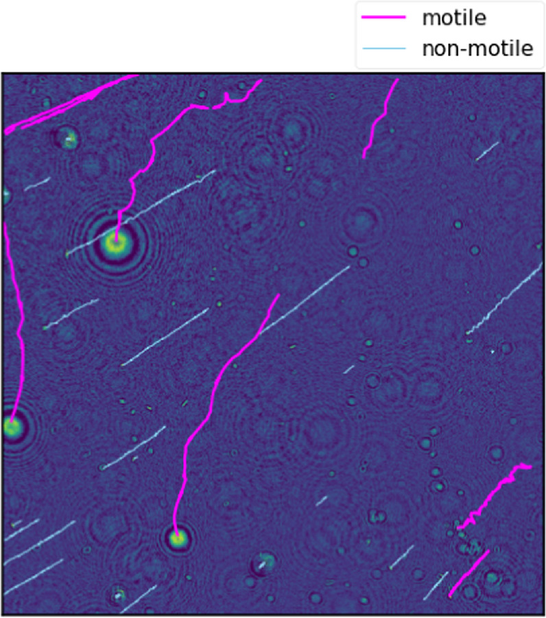
Figure 13. The tracker identifies particles and links them through time to form tracks. Here, tracks are overlaid on the 80th frame of a DHM observation. ML-derived motility classifications are indicated by track color. Tracks classified as motile are magenta while tracks classified as nonmotile are blue.
Download figure:
Standard image High-resolution imageTo assess how tracking performance was affected by particle density and SNR, we generated 360 simulated studies spanning three particle density levels and six SNR levels (Figure 14). Higher amounts of particle overlap (e.g., resulting from crowded scenes) led to substantial degradation in tracker performance. This indicates that tracking is limited in observations with many particles even if those particles are visually obvious against the background. In general, once SNR crosses above approximately 0.5, it has a relatively small effect on tracker performance in crowded scenes. For uncrowded and semicrowded scenes, increasing SNR confers a steadier increase in performance. Experimentally, these results indicate that the capability to dilute water samples (to reduce particle density) is important to ensure optimal particle tracking.
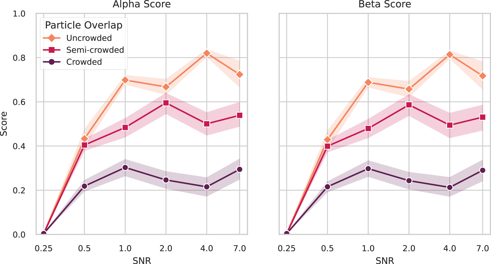
Figure 14. Tracking performance increases with SNR and decreases with particle density. However, changes are limited above SNR = 0.5 for the crowded observations, consistently resulting in a >50% reduction in tracking performance. Note that the maximum value of the beta metric is the alpha metric.
Download figure:
Standard image High-resolution image5.6.2. Motility Classifier Performance
We evaluated three ML architectures for classifying track motility: GBTs (Friedman 2001), RFs (Breiman 2001), and SVCs (Cortes & Vapnik 1995). These methods were chosen for their simplicity, interpretability, and the computational efficiency of their Scikit-learn implementations (Pedregosa et al. 2011). We used five-fold stratified cross-validation to iterate over different combinations of the labeled data (Section 4.1) while avoiding data leakage from highly similar experiments. We also applied Bayesian optimization to optimize each method across its hyperparameter search space. 6 Each model was optimized to maximize the area under the receiver operating characteristic curve (AUC ROC). AUC ROC was chosen for its ability to represent the precision-recall trade-off; with a model that performs reasonably over a range of posterior probability thresholds, ground teams can make an informed trade-off between conserving data bandwidth and missing a low-confidence motile organism. For a specific flight mission implementation, this tuning would be thoroughly re-examined.
Figure 15 shows the performance of each optimized model architecture using precision-recall and decision error trade-off (DET) curves, which assess binary classification performance over a range of decision thresholds. Precision-recall curves represent the trade-off between the two metrics and are especially informative if the data set contains a class imbalance. DET curves provide the same information as an ROC curve, but at a scale that better highlights cross-model performance differences and explicitly represents the trade-off between false positives and false negatives for a range of probability thresholds (Martin et al. 1997). In both representations of model performance, the RF and GBT models surpass the SVC model. The GBT, RF, and SVC models achieved AUC ROCs of 0.88, 0.92, and 0.86, respectively. RF reaches the higher overall F1-score (the arithmetic mean between precision and recall) of 0.78, compared to 0.71 and 0.63 for the GBT and SVC, respectively. A different Fβ score may be used to evaluate different precision/recall trade-offs as desired. Elapsed ML prediction times for all models were well below 1 s, but the GBT and SVC architectures were approximately 75 × faster than the RF (see Table 5 for onboard runtimes). Due to the classifier performance and acceptably short runtime, we selected the RF model for further analysis.
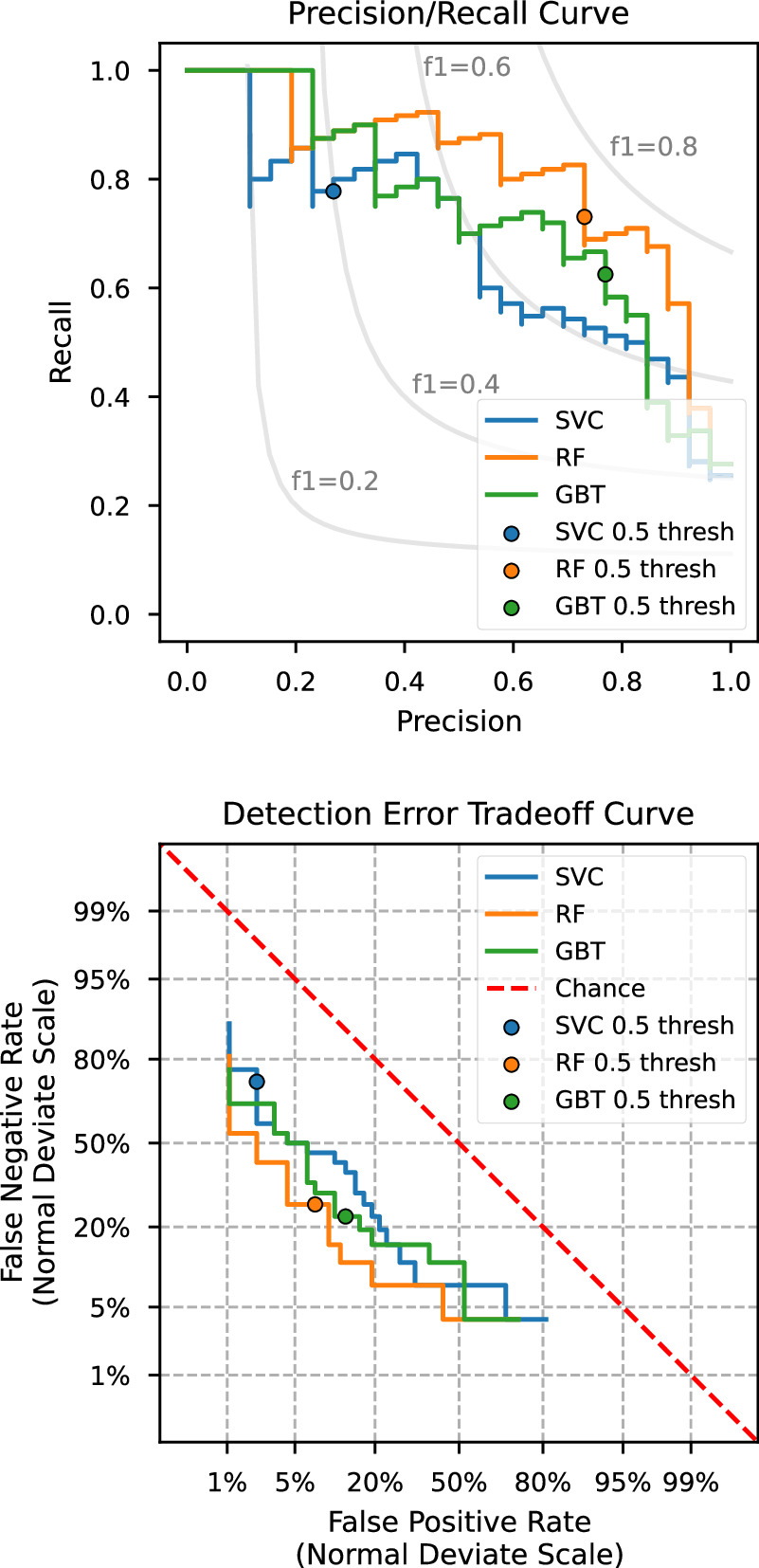
Figure 15. We evaluated the performance of three classical ML models for identifying motility on a held-out test set: SVC, RF, and GBT. Top: precision-recall curve displays the balance between these two metrics. Here, perfect performance corresponds to the top-right corner. The circular marker on each classifier trace corresponds to a 50% confidence threshold. Bottom: DET curve displays the balance between false negatives and false positives when traversing a range of confidence thresholds. Perfect performance corresponds to the lower-left corner.
Download figure:
Standard image High-resolution imageTo interpret how individual features (track extracted variables) contribute to classifier decisions, we applied the ML explainability method Shapley additive explanations (SHAP) to our trained RF model. SHAP uses a game-theoretic approach to estimate the role of each feature in individual predictions (Lundberg & Lee 2017). Figure 16 shows the SHAP values for the 10 most impactful features used by the RF model. Here, negative SHAP values (left of center) indicate data points where the feature value corresponded to a push toward nonmotile predictions, while positive values (right of center) indicate tracks where the feature value corresponded to a push toward a motile prediction. For an intuitive example, tracks with a low mean speed or relative speed—indicating tracks that moved slower overall or relative to other tracks in the same observation—translated to lower motility probability as indicated by the concentration of blue points to the left of center.

Figure 16. Track features contribute to the motility prediction in different ways, but relative and directional features were frequently ranked among the most important. Using SHAP, this plot illustrates how the 10 most impactful features (shown in descending order) contribute toward the RF model's final motility predictions. For each feature row, the corresponding impact of each feature on the final decision is shown for all tracks (each plotted as one point per row). Note that more important features tend to have wider distributions (along the horizontal axis) corresponding to larger effects on the output probabilities. The color of the points indicates whether a specific track's feature was relatively high or low compared to all others. Taken together, this visualizes how track features contributed to the output classification decisions.
Download figure:
Standard image High-resolution imageIn general, the classifier used a variety of different feature types to make decisions. Relative features, which quantify how similar or dissimilar a track was compared to the population of other tracks in the observation, make up the top two features. This highlights the importance of comparing each track against other tracks observed at the same time. High values for relative step angle, which implies a track changed direction much more than other observed tracks, corresponded to a strong push toward motile predictions. For relative cosine similarity, high feature values—implying the end-to-end track direction was nearly identical with other tracks—tended to correspond to nonmotile predictions. The importance of relative features in classification decisions also implies the existing system is likely to perform worse for (1) extremely sparse observations where only a single track is observed or (2) cases where multiple motile cells move in unison (similar to a school of fish). Interestingly, "standard" metrics related to speed and acceleration (see Section 3.3.3) were of limited importance; only two of the 10 calculated ranked among the top 10. Others have noted that this line of explainability analysis, seeking to characterize precisely how the model makes its determinations, is a vital step toward gaining mission inclusion because it helps build trust with all stakeholders through familiarity and intuition (Slingerland et al. 2022).
Section 3.3.4 described how the classifier's posterior probabilities may be used for downlink prioritization. To validate the model outputs, we conducted a calibration assessment by binning posterior probabilities from the test set and checking if the percentage of truly motile tracks aligned with the model's predictions. Since each model appears under- or over-confident for certain portions of the predicted probability, we applied model calibration to adjust their output probabilities. Figure 17 shows the original (uncalibrated) and calibrated GBT, RF, and SVC models on the held-out test set. Here, cross-validated isotonic calibration was applied, but other methods also exist. While the application of calibration improves model outputs to more closely match the diagonal line (corresponding to ideal performance), some under- and overconfidence remains. Regardless of whether or not the calibrated model is used in a mission scenario, this procedure improves transparency and interoperability by exposing how faithfully an ML model's probability estimates align with reality based on the training/validation data available to the system. Note that calibration functions are strictly monotonic, and therefore do not impact model performance metrics shown in Figure 15. Taken together, these results demonstrate that the motility classifier meets requirement L4-3 in Table A3, with both satisfactory classification performance and estimation of probability of lifelike motility.
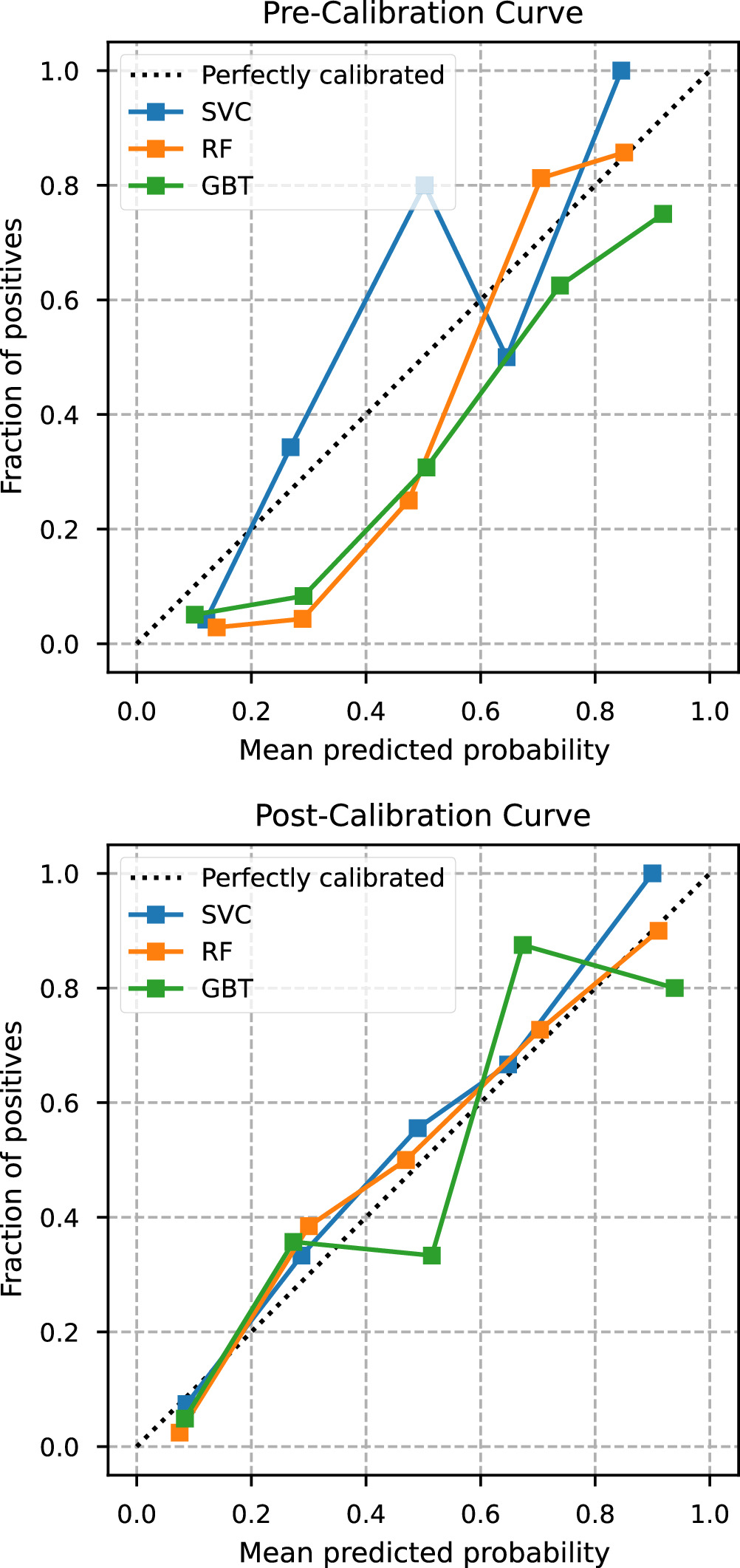
Figure 17. Model calibration provides a mechanism to correct bias in our trained motility classifiers and normalize to a true empirical likelihood estimate. Top: uncalibrated GBT, RF, and SVC classifiers generate predicted probabilities that do not always align with the true class on a held-out test set. Points above the diagonal line indicate low confidence, while points below the diagonal line indicate overconfidence. Bottom: after cross-validated, isotonic calibration the model outputs more reliably represent the true probabilities within each bin.
Download figure:
Standard image High-resolution image
5.6.3. Particle Portraits
While raw DHM and FLFM observations are much too large to transmit from ocean worlds, HELM and FAME crop small, full-resolution particle "portraits" to extract the raw image data containing tracked particles (as discussed in Section 3.3.5). Scientists can reconstruct these portraits to different z-planes and analyze morphology or search for subcellular structures in any suspected microorganisms. Since the reconstruction algorithm is computationally expensive (see Section 2.2) and the space of possible particle morphologies is difficult to analyze autonomously with OSIA, we include these particle portraits in the downlinked ASDPs for manual investigation by science teams. Figure 18 shows two example reconstructions from Mono Lake data. While the microorganisms identified during the field campaign were small, spherical, and displayed no obvious subcellular details, this capability to extract individual particle sizes would provide valuable detail for microorganisms with nonspherical shapes or resolvable subcellular structures.
Figure 18. Image reconstructions allow for detailed analysis of individual microorganisms. The reconstructions here were generated using particle portraits extracted from tracks identified at Mono Lake and show DHM (left) and FLFM (right) images refocused to the depth of the contained particle. The small, central white dot in the left image shows the microorganism responsible for the zig-zagging movement pattern in Figure 7 while the right image shows one of the autofluorescent particles belonging to the rare particle class hypothesized to contain green fluorescent protein. This figure is available as a 3 s animation, which steps through the full z-stack of focal reconstructions to convey the 3D structure of each particle.
(An animation of this figure is available.)
Download figure:
Video Standard image High-resolution image
6. Infusion and Adoption
Life detection is an important theme for several mission concepts in the most recent Planetary Science Decadal Survey (National Academies of Sciences, Engineering, and Medicine 2023). To enable unambiguous life detection, these missions should include multi-instrument payloads like OWLS that collect observations relevant to multiple orthogonal biosignatures. Many of these instruments produce large data volumes and could benefit from the type of OSIA treatment described in this work. In this Section, we seek to directly inform mission formulation to encourage early consideration of these onboard science capabilities. Specifically, we will review potential benefits to consider during formulation trade studies, assess the computational feasibility of OSIA for three life detection concepts, and identify future ConOps tools needed to successfully deploy OSIA. Finally, we will discuss lessons learned through this work and highlight terrestrial science applications that could be leveraged to further mature these novel capabilities for space flight infusion.
6.1. OSIA for Mission Concepts
In Section 1.4, we discussed how OSIA can improve a mission's science return through summarization and prioritization, alleviating the bandwidth barrier often facing planetary missions. To illustrate the impacts of this improvement, we reference our OSIA implementation on OWLS to estimate how OSIA could benefit three relevant life-detection mission concepts.
6.1.1. OSIA Enabled Capabilities
Onboard science capabilities may be developed to achieve a variety of goals. We will explore six here: addressing data sufficiency, supporting advanced instruments, leveraging inactive periods, shortening reaction times, retargeting/reprocessing observations, and improving communication robustness. While we discuss these at a high level, detailed, formulation trade studies are needed to both identify which (if any) of these advantages warrant OSIA consideration and to quantify any expected benefits. We acknowledge that, for each of these capabilities, additional constraints and considerations such as available power, thermal management, and consumable resources such as sampling vessels, time to physically collect samples, and competing instrument observation schedules will ultimately influence infusion. Some of these concerns may be addressed by integrating synergistic autonomy elements such as onboard planning and scheduling (Gaines et al. 2022).
Data Sufficiency—For any new mission concept, mission architects must show how the volume and type(s) of observational data collected will address the scientific questions at hand. OSIA offers an alternative to the standard practice of transmitting all collected raw instrument data. For example, mission teams may wish to acquire more observations than can be downlinked when searching for rare phenomena and then only transmit those deemed scientifically useful. Alternatively, for a fixed bandwidth, missions can transmit summaries of many more observations than would be possible if returning raw data. Here, a simple metric of success could compute the ratio of total time spent returning an observation to the team (processing + transmission) for traditional and OSIA-based approaches (as we do later in Section 6.1.3).
Advanced Instruments—The combination of OSIA and next-generation processors will enable the consideration of newer, high data volume instruments that are infeasible for today's planetary mission concepts. Such was the core benefit provided by HELM and FAME—summarization of high-resolution video enables the search for cellular motility even when exploring bandwidth-constrained science targets like Europa and Enceladus. This mismatch between data collection and data downlink rates also limits the use of other advanced instruments such as high-resolution imaging spectrometers or Raman spectrometers. The combination of both OSIA and next-generation processors is likely required for deployment of these instruments beyond Earth's orbit. Modern multispacecraft concepts (e.g., cubesat constellations or distributed landers) may also face a similar challenge as their collective data volumes can outstrip today's monolithic spacecraft. When considering OSIA, an early metric of success might be to simply assess feasibility; for a given communication bandwidth, concept teams could determine if OSIA could conceivably summarize these large observations to fit within bandwidth constraints.
Leveraging Inactive Periods—Missions may include periods of inactivity due to communication downtime or limited observation opportunities. These idle periods may be reclaimed for observation processing to summarize and/or prioritize previously acquired observations for upcoming communication windows or other autonomously triggered tasks. This could substantially increase the number of observations returned by reducing or eliminating the impact of OSIA processing on "active mission time." Such was the primary benefit of the AEGIS algorithm deployed on the Curiosity and Perserverence rovers (discussed in Section 1.5), which selects rocks for ChemCam sampling after a drive but before a ground-in-the-loop command cycle (Francis et al. 2017). One useful metric of success here might be the number that additional science data returned when comparing a manually commanded spacecraft to one with OSIA.
Faster Reaction Times—The time required to transmit, process, and review raw observations during traditional "ground-in-the-loop" cycles limits the agility of mission teams. Current missions do not determine transmission order according to an onboard estimate of scientific utility; raw data requires (sometimes extensive) ground processing before reaching science teams, and spacecraft cannot often react autonomously to scientific data even if other autonomous systems are in place (e.g., for planning and scheduling). Thus, reactions to instrument data or problems can be delayed to the point of irrelevance. OSIA's ability to assess observations onboard means transmitted data can directly inform ground teams about the state of the scientific environment, thereby permitting faster decision making. It also opens the possibility for more missions to make autonomous decisions based on science data. A simple proxy metric for evaluating OSIA might be the reduction in time required to alert ground teams to phenomena of interest.
Soft Retargeting and Reprocessing—When data summarization involves excising regions of interest from the original observation (either autonomously as with HELM and FAME or via manual specification), there is the risk of omitting scientifically interesting content. By storing the raw data onboard and supporting reconfiguration of the OSIA, observations may be reprocessed to better extract the desired content without re-acquiring each observation. Similarly, OSIA parameters may be updated to improve summary products and optimize science utility on previously processed raw observations. For this benefit, a possible metric of success is the total number of unique observations that are processed and transmitted to ground. With retargeting and reprocessing, repeat observations (e.g., to correct issues with an initial observation) should be reduced, so the spacecraft can spend more resources sampling the environment for new phenomena.
Communication Robustness—To receive instrument data, transmissions from spacecraft beyond Earth's orbit must go through the Deep Space Network (DSN). Therefore, a mission's science yield may be affected if those assets do not meet the availability that was envisioned during formulation. For example, increased rationing of DSN downlink time during upcoming crewed Artemis missions or malfunctions in one of the aging Martian relay orbiters could impact the transmission viability of interplanetary missions. Where appropriate, OSIA is worth exploring as a tool to improve communication robustness during such situations; the capability to prioritize transmission of data with the highest estimated science utility or tune OSIA configuration to summarize more aggressively may mitigate mission risks. A method to quantify any benefits might involve first collecting (or simulating) a set of representative instrument data. Using this data set, a mission formulation team could estimate how science return is affected under a set of increasingly strict bandwidth constraints for conventional versus OSIA-based processing approaches.
6.1.2. OSIA Feasibility on Flight Processors
A critical consideration for the infusion of any OSIA is compute feasibility. For some mission concepts, advanced compute resources will be required to enable the autonomy algorithms developed in this work. To inform this need, we provide coarse feasibility estimates for OSIA on future missions by considering how the runtime of our algorithms will change depending on the compute platform available. We acknowledge that, short of benchmarking a skillfully ported algorithm to a specific flight compute architecture, cross-processor comparisons are difficult to estimate accurately. Therefore, we limit these analyses to an order-of-magnitude (OOM) estimate.
We broadly divide our compute comparison into current- and next-generation processors. The first category of processors we consider are those with clock speeds in the 100 MHz range; this includes the RAD750 and LEON class of processors. The RAD750 was deployed on Mars Science Laboratory (MSL) (Curiosity) and M2020 (Perseverance) while LEON processors were used on the LICIACube satellite, which observed DARTs asteroid impact, as well as a number of Low Earth Orbit (LEO) CubeSats. The second category consists of processors with clock speeds in the 1 GHz range, including the Snapdragon 855 and High Performance Space Computer (HPSC). The Ingenuity helicopter uses an earlier Snapdragon model (the 801), but note that the HPSC has not been deployed as it was in development as of the time of this work. A previous study by the NEAScout mission quantified onboard science processing performance changes across these two processor classes (Lightholder et al. 2023a). A variety of compute operations demonstrated runtime improvements on the order of 10 × to 220 × (with a total improvement of 50 × ) when moving from megahertz- to gigahertz-scale processors. Using this analysis, we provide tentative predictions about the runtimes of HELM and FAME on future missions.
If deployed, we expect that a flight implementation of our OSIA algorithms will run at least as fast on a dedicated gigahertz-scale processor (e.g., the Snapdragon 855) as on the i7-3612QE third-generation quad-core processor used in our field trial, as benchmarked in Table 5. This is a reasonable assumption as: (1) we expect that a compiled flight-ready implementation of our software will run faster than the current implementation in Python (an interpreted language), (2) the Snapdragon 855 has a faster base frequency (2.96 GHz) than the i7 processor (2.1 GHz), (3) the Snapdragon 855 has eight physical cores compared to the i7 processor's four (hyperthreaded to eight), and (4) the Snapdragon 855 has hardware accelerators (including a Graphics Processing Unit (GPU)) that could further accelerate image processing steps used on HELM and FAME. (The i7's integrated HD4000 GPU was not used in this work). Therefore, we can conservatively estimate that HELM's and FAME's per-observation processing time will remain in the hundreds of seconds for gigahertz-scale compute platforms (as quantified in Table 5). Further, we take the most conservative conclusion from Lightholder et al. (2023a) and estimate a 10× slowdown for megahertz-scale compute platforms, estimating a runtime of thousands of seconds for this category. Beyond processor considerations, HELM and FAME were designed with RAM, storage, and runtime constraints in mind. Software configuration allows mission operators to adjust parallelism to take advantage of platforms with extensive hardware resources (RAM and CPU cores), while still operating on platforms with limited resources. We acknowledge that many other factors affect compute time, and other mission constraints and risk posture will limit choices around flight processors. Regardless, these estimates indicate that OSIA algorithms described in this work could be feasibly deployed on either megahertz- or gigahertz-scale compute platforms.
Table 6. Coarsely Estimated OSIA Runtime on Flight Processors
| MHz Scale a | GHz Scale b | |
|---|---|---|
| Clock Speed (MHz) | 100 s | 1000 s |
| Typical RAM | MBs | GBs |
| Avail. Hardware Accel. | N | Y |
| OOM Time per Sample | 1 × 10³ s | 1 × 10² s |
Notes. Considering megahertz- and gigahertz-scale processor performance and our OSIA implementation on the field computer (Table 5), we limit our estimate of HELM's and FAME's observation processing time on flight computers to an OOM.
a RAD750, LEON-class (Själander et al. 2009; Berger et al. 2001; Lightholder et al. 2023a) b Snapdragon 855, HPSC, (Doyle et al. 2013; Balaram et al. 2018; Powell 2018; Dunkel et al. 2022)Download table as: ASCIITypeset image
6.1.3. Potential Impacts on Mission Concept Formulation
Existing reference mission concepts aimed at detecting life in our solar system vary greatly in terms of their constraints and proposed ConOps. Therefore, it is illustrative to explore how OSIA might impact each. We refer to OSIA capabilities outlined in Section 6.1.1 below, but we emphasize that complete formulation trade studies are needed to precisely quantify any potential benefits. Such a study must consider other critical choices (e.g., available power, thermal management, consumable resources, scheduling, sample collection). While a full trade study is beyond the scope of this work, we highlight how OSIA can enhance the architecture or operations of existing mission concepts. To support this analysis, we will refer to Table 7, which calculates the time-to-ground speeds for computing and downlinking ASDPs compared to the more conventional approach of downlinking raw data after ZIP compression. We also continue our focus on microscopes for biosignature detection, but the benefits of science autonomy for other instruments are discussed elsewhere (Francis et al. 2017; Mauceri et al. 2022; Theiling et al. 2022).
Table 7. Coarse OOM Estimates for Time-to-ground Speed-up Ratios of a Single DHM Observation (Defined in Section 4 and Table 4) for Three Mission Concepts, Two Processor Categories, and Using HELM Summarization (ASDPs Produced by the "High-bandwidth" Configuration) or ZIP Compression
| Ref. Mission | ZIP product | ASDP | MHz Scale | GHz Scale |
|---|---|---|---|---|
| (Downlink Rate) | Downlink (s) | Downlink (s) | OOM Speed-up a | OOM Speed-up b |
| Enceladus Orbilander (34 kbit s−1) | 2.6 × 10⁵ | 3.4 × 10² | ≈2 | ≈3 |
| Europa Lander (48 kbit s−1) | 1.8 × 10⁵ | 2.4 × 10² | ≈2 | ≈3 |
| Martian Rover (1000 kbit s−1) | 8.8 × 10³ | 1.2 × 101 | ≈1 | ≈2 |
Notes. While these estimates provide rough intuition for how to compute platforms and the inclusion of onboard processing may benefit science return, a thorough mission architecture trade study must consider many other constraints to evaluate the true impact on any mission concept. Estimated OSIA runtimes are from Table 6.
a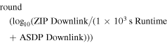 b
b
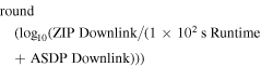
Download table as: ASCIITypeset image
Enceladus Orbilander—The Enceladus Orbilander (MacKenzie et al. 2021) is a concept with potential OSIA applications driven by its extreme distance and relatively long duration of 2 yr. While at Saturn, the concept estimates a science data downlink rate limited to 34 kbit s−1. It describes the deployment of a Life Detection Suite (LDS) similar to OWLS, and includes a microscope as a high-risk, high-reward instrument. Over the course of 2 yr of surface operations, the mission concept specifies 29 microscope observations totaling 0.12 GB of data, and would collect only still images to directly look for cells.
In this case, potential OSIA applications are driven by the 2 yr surface phase. This affords considerable onboard processing time, meaning that a less-powerful onboard processor may be permissible given ample inactive periods to process each observation. As seen in the first row of Table 7, OSIA with a megahertz-scale processor would still provide a two OOM speed-up over downlinking raw compressed products. As samples are collected passively (dependent on fallout and accumulation rates) or actively (dependent on scooping material from the surface), OSIA alone would not enable additional sample collection. However, multiple observations per physical sample could be enabled. Each would then be analyzed and down-prioritized to reduce scientifically redundant information to improve data sufficiency. Additionally, OSIA could better inform follow-up sample collection. For example, the "LDS Full" operational mode specifies two separate sample scooping procedures. Expedient, prioritized return of summarized ASDPs from the initial observations could inform reactive decisions about when and where to collect the second scoop. Finally, the three OOM speed-up afforded by more powerful onboard computation would enable advanced instrument observations such as microscopy videos. This could enable the search for motility biosignatures as demonstrated with HELM and FAME.
Europa Lander—The second reference mission is the Europa Lander mission concept (Hand et al. 2022) with OSIA applications driven by its substantial distance, short mission duration of 30 days, and a desire for a combination of autonomous operations and decision making by the ground science team. The concept describes a baseline model payload that includes optical and atomic force microscopes and plans for only five total samples. Communication bandwidth is estimated at 48 kbit s−1, which would be shared between science and telemetry. The authors noted in a previous concept that the communication rate could "represent the biggest bottleneck in the timely return of decisional data" (Hand et al. 2017). The latest concept specifically discusses autonomy to address this issue, including "autonomy and machine-learning techniques...to allow the onboard system to replan communications activity, based on assessment of instrument data and priority measurements" (Hand et al. 2022).
With an expected combined science and engineering data return of >187.5 MB over the 30 day mission, data sufficiency and communication robustness are important considerations for this mission concept. Compared to the planned approach of raw-data transmission, OSIA's ability to summarize and prioritize data could improve the chances that any encountered biosignatures are successfully transmitted. As in the second row of Table 7, OSIA with a gigahertz-scale processor would provide a three OOM speed-up over downlinking raw compressed products. In addition, the short lifetime of the mission implies that operators will be under significant time pressure for any ground in the loop operations. Therefore, the rapid transmission of any summarized scientific insights is likely to be valuable for informing and shortening decision-making processes. The mission concept also states that, due to the constraints of direct to Earth communication, there would be significant idle time on the surface of Europa, which could not be utilized without autonomy (Hand et al. 2022). Finally, as with the Enceladus Orbilander concept, OSIA would enable advanced instruments (such microscopy videos for motility assessment) without significantly increasing downlink bandwidth or requiring new samples. For a mission as sample- and time-limited as Europa Lander, an additional biosignature capability could translate to a meaningful improvement in life detection sensitivity.
Martian Rover—The final reference mission we consider is a Martian rover (similar to Curiosity or Perseverance) focused on life detection. We include this reference to evaluate OSIA benefits for a relatively close, high-bandwidth mission. Current rovers like Curiosity and Perseverance depend on orbiters (Mars Reconnaissance Orbiter (MRO), Odyssey, Mars Atmosphere and Volatile Evolution (MAVEN), and ExoMars Trace Gas Orbiter (TGO)), to support their data transmission, which ranges from 8–2048 kbit s−1 (Gladden et al. 2022). For the sake of this estimation, we will consider an average data rate of 1000 kbit s−1.
OSIA inclusion on this future Martian rover concept would be driven by the need to support a daily operations planning cycle. Here, the mission cadence is likely to be similar to past rovers involving a sequence of detailed site explorations with short drives between each. While rover planning teams will not regularly face planning cycles as consequential as on Europa Lander, reaction time is still a concern. The ability to rapidly return a few summary data products could guide mission teams to better optimize where and how they spend resources when searching for biosignatures. This reduces the risk that a sample site is abandoned prematurely or that valuable mission time is squandered at a site of low scientific value. OSIA also offers the chance to collect many observations and leverage soft retargeting to analyze collected data over a long time period. Longer drives, for example, may leave substantial inactive time for iterative OSIA analysis of previously collected observations. As seen in the third row of Table 7, OSIA with an existing megahertz-scale processor would provide an OOM speed-up over downlinking raw compressed products. This would be advantageous if the mission chose to collect data at high rates while at a site of interest, then process and transmit data during the upcoming drive. OSIA may also provide communication robustness if there are any malfunctions in the orbital relay network, which would otherwise unexpectedly limit the rate and/or cadence of data transmission. Given the relatively high data bandwidth, a Mars mission may also be the most likely to deploy advanced instruments like Raman or imaging spectrometers. Overall, OSIA may offer some enhancements and risk reduction for a future rover concept, but the advantages are not as enabling compared to the Enceladus Orbilander and Europa Lander concepts exploring the outer solar system.
Ultimately, we seek to inform mission concept teams how processor choice and the presence or absence of OSIA will impact science return. By comparing the combined runtime and transmission time of different strategies, Table 7 displays the estimated OOM change in an observation's time-to-ground given choices in available data processing techniques (simple ZIP compression or OSIA) and available compute platforms (megahertz- or gigahertz-scale; Table 6). At a high level, this analysis indicates that OSIA has the greatest potential benefits for missions with low downlink bandwidth and a next-generation, gigahertz-scale processor. For missions with high bandwidth, OSIA's potential benefits are diminished as the onboard runtime becomes a significant component of the total processing and transmission time. Regardless of the processor choice, we estimate that OSIA will provide at least one OOM speedup in data return, which translates to either reduced time for a set data volume to reach ground teams or the ability to transmit a larger number of summarized observations in a fixed time window. Note that while we isolated these two aspects of the trade space for clarity, a true mission architecture study must explore a multitude of interconnected design choices simultaneously.
6.2. Path to Flight: Concept of Operations
Given the fundamentally unknown nature of extraterrestrial life, the pursuit of biosignatures will require a nimble interaction between science teams and the OSIA. The autonomy must therefore be capable of reconfiguration mid-mission to emphasize certain signals of interest and de-emphasize environmental distractions. This implies a new, more nimble ConOps strategy than is typically used today. For existing OSIA demonstrations such as AEGIS, reconfiguration is treated as a rare event that requires extensive manual effort by the original research team, usually in response to data quality degradation. Moving forward, mission-enabling OSIA will necessitate a more principled reconfiguration process: one that transparently captures new science intent, can be completed in hours or days, and produces reproducible, statistically defensible OSIA configurations.
The defining novelty of OSIA ConOps is the specification of its goal-based behavior rather than manually defined, imperative commands. In this regime, future operators will focus on selecting OSIA configuration parameters that produce desirable outcomes for a statistically majority of the expected, future instrument observations. They will rely on new ground software tools to search this space of possible OSIA configurations, likely observations, and their evaluated OSIA outcomes to inform the selection of a single configuration that best matches the current science intent. This challenge and its solution are similar to mission formulation trade studies, where ensembles of simulations are routinely used to evaluate and select potential designs versus predicted science outcomes. We are currently developing an open prototype of such a ground tool called the Data-driven Efficient Configuration of Instruments by Scientific Intent for Operational Needs (DECISION; Lightholder et al. 2023b), scheduled for completion in 2024.
6.3. Early Integration of Science, Instrument, and Autonomy Teams
OSIA development is inherently interdisciplinary and therefore hinges on a strong collaboration between multiple stakeholders: the OSIA developers themselves, science domain experts, instrument developers, and flight hardware and software teams. The practice of spiral development was used to facilitate this early interaction, which we describe with greater detail in Slingerland et al. (2022). Initially, the autonomy team focused on a minimal end-to-end solution containing all of the critical OSIA modules as described in Figure 4. After finishing a simple, working version of HELM and FAME, the team held biweekly feedback meetings with scientists and instrument developers to review results, identify outstanding challenges, and prioritize improvements in the hardware, algorithms, or observational data record. This accelerated development for all parties involved. For example, early MHI and frame-to-frame pixel difference plots helped to identify and characterize instability in sample fluid flow (due to occasional clogs). In another case, the dropped frame validation check identified that extraneous background processes were occasionally overloading the flight computer early in F-Prime integration. These examples illustrate the advantages of integrating OSIA early in development to increase system-level awareness and inform problem-solving across the mission. This approach is novel in the current mission environment where software and hardware teams are typically siloed until late-mission integration and testing.
To engender trust with the science, instrument, and flight hardware teams, we deliberately regulated the complexity of the OSIA's underlying algorithms. Through repeated interaction and negotiation, we observed that simpler algorithms helped us better engage with the science team during spiral development, provide interpretable explanations of the OSIA's decisions, and meet timeliness requirements using the limited onboard compute resources available. Specifically, the choice of the LAP tracking algorithm was influenced by existing science domain expert familiarity. Similarly, classical ML models (e.g., RFs and GBTs) were selected for their explainability and relatively low compute requirements. While larger, more sophisticated algorithms such as convolutional neural networks or auto-encoders may bring certain performance advantages, they are also "black-box" models that are harder to interpret, require much more data to train, and use significantly more compute resources. Therefore, we chose not to rely on large or complex algorithms (such as deep learning models) as they would make for a poorly behaved citizen within the OWLS onboard ecosystem.
6.4. Additional HELM and FAME Applications
Beyond the planetary life detection context, HELM and FAME hold promise for many other use cases driven by their ability to systematically and efficiently process large numbers of microscopic observations (Reimer et al. 1997; Sweeney et al. 2019). Some of these applications could also serve as useful opportunities to mature our systems for mission application. For example, automatically identifying motility styles could directly inform large-scale oceanic bacterial catalogs (Grossart et al. 2001; Mullen et al. 2020; Dinasquet et al. 2022), both to categorize known species and identify novel organisms. Low-cost, submersible DHMs are actively being developed for this purpose (Ramirez et al. 2022). For more direct societal impact, applications such as food safety analysis as well as beach and flood water safety are currently performed by manual motility inspection, as are the quantification of antibiotic efficacy and sepsis diagnoses (Leonard et al. 2003; Lazcka et al. 2007; Saxena et al. 2014; Valderrama et al. 2015; Martin et al. 2016; Park et al. 2018; Shahraki et al. 2019; Tomenchok et al. 2020; Cholewińska et al. 2022). Like our field trial use-case, the driving need in these terrestrial applications is guiding human attention to the most relevant data through summarization and prioritization. But whether at home or at interplanetary distances, limited by communication bandwidth or human attention, the most impactful role for OSIA remains as a tool to help diagnose, discover, and understand the wealth of complex data that now surrounds us.
7. Funding
The research was carried out at the Jet Propulsion Laboratory, California Institute of Technology, under a contract with the National Aeronautics and Space Administration (80NM0018D0004).
Acknowledgments
This research occurred at the Jet Propulsion Laboratory, California Institute of Technology, under a contract with the National Aeronautics and Space Administration. We acknowledge the entire OWLS team, especially Andrew Berg, Michael Starch, Santos "Felipe" Fregoso, Aaron Noell, Gene Serabyn, Emily Dunkel, Shawn Anderson, Zaki Hasnain, Ravi Kiran, Peyman Tavallali, and Marc Foote. We would also like to acknowledge Mae Dubay, Nikki Johnston, and Max Riekeles as well as the two anonymous reviewers for providing useful insights. Data annotation for this project was provided by contractors Aman Kumar, Sonali Jain, Aman Sajwan, Bittu Kumar, and Waseem Khan through Labelbox, Inc.
© 2024. All rights reserved.
Disclosures
The authors declare no conflicts of interest.
Appendix
: Field Test Requirement Tables
We developed mission-like, OSIA-focused requirements to guide the design, development, and evaluation of the algorithms discussed. These notional requirements are also meant as an example for future OSIA-enabled missions (Tables A1–A3).
Table A1. OWLS Field Test Level 1 and 2 Requirements Relevant to HELM/FAME
| Level | Short Name | Requirement | Justification |
|---|---|---|---|
| L1 | Autonomous Life Detection | The OWLS suite shall autonomously investigate samples for molecular and cellular evidence of life in naturally occurring ocean-world analog environments. | Top level driving science capability. |
| L2 | Science Autonomy | The OWLS Project shall summarize and prioritize observations from multiple samples for downlink to maximize returned evidence for life. | Limited data bandwidth and long communication delays prevent the return of most raw data and rapid ground-in-the-loop commanding. |
Download table as: ASCIITypeset image
Table A2. OWLS Field Test Level 3 Requirements Relevant to HELM/FAME
| Level | Short Name | Requirement | Justification | Conf. |
|---|---|---|---|---|
| L3-1 | Data Summarization | The OSIA shall produce reduced data volume science products to characterize biosignatures while meeting the total baseline mission data budget. The data reduction ratio against the raw data volume shall be at least 1000 × . | While we prescribe this requirement for the field test, observations in deep space mission concepts may be up to 10,000 times larger than available downlink bandwidth. | Demo Section 5.2 |
| L3-2 | Data Prioritization | The OSIA shall rank order science data products by their anticipated scientific value. | Missions may collect more observations than can be returned even with summarization capabilities, and data downlink may also be interrupted or delayed. Therefore, transmissions should include the most compelling products first at each opportunity. | Demo Section 5.3.3 |
| L3-3 | Computation | The OSIA shall complete all necessary validation, summarization, and prioritization using available flight computing resources within the acceptable timeliness window. | Flight computer capabilities and power budgets place significant restrictions on OSIA algorithms. | Demo L4-7 |
| L3-4 | Operational Monitoring | The OSIA shall generate engineering telemetry sufficient to substantiate nominal operation of the autonomy and monitor instrument data quality. | The autonomy must support scientific conclusions with transparent, traceable behavior and provide operational parameters that can be trend-analyzed and tracked in the established mission operational paradigm. | Demo Section 5.1 |
| L3-5 | Reconfigurability | OSIA's behavior shall be controlled by configuration files that may be updated during the mission to optimize its behavior. It shall generate data products sufficient to detect the need for and inform reconfiguration. | The science operations team must have some awareness of nonprioritized observational contents to preserve the discovery of the unexpected as well as enable reconfiguration to pursue an evolving science focus or adapt to changing instrument behavior. | Demo Section 5.1 |
Note. The confirmation method "Demo" refers to the inspection, analysis, demonstration, and test (IADT) equivalent.
Download table as: ASCIITypeset image
Table A3. OWLS Field Test Level 4 Requirements Relevant to HELM/FAME
| ID | Short Name | Requirement | Justification | Conf. |
|---|---|---|---|---|
| L4-1 (L3-1,2) | Particle Tracking True Positives | HELM and FAME shall produce science data products that detect and track Well Resolved Targets and their motion within an Uncrowded Observation (raw image sequence versus time) with at least 50% True Track Coverage. | Capable particle tracking is needed for biosignature summarization and prioritization. Increasing sensitivity improves this metric but incurs more false positives. | Demo Section 5.6.1 |
| L4-2 (L3-1,2) | Particle Tracking False Positives | HELM and FAME shall produce science data products that contain less than 10 False Track Points per Uncrowded Observation frame. | Performant particle tracking generates fewer false positive detections per frame to prevent crowding out of true biosignatures during downlink prioritization. Reducing sensitivity improves this metric but incurs more false negatives. | Demo Section 5.6.1 |
| L4-3 (L3-1,2) | Motility Identification | HELM and FAME shall produce science data products that estimate the Empirical Probability of Life-Like Motility for each identified Well Resolved Target to inform summarization and prioritization. | The threshold for lifelike detection should be interpretable to the science team, not arbitrary in units or meaning. | Demo Section 5.6.2 |
| L4-4 (L3-1,2) | Fluorescence Identification | FAME shall produce science data products that track and characterize each Well Resolved Target in FLFM observations to inform summarization and prioritization. | Regardless of motility, information about any fluorescent particles (either innate or dye-induced) is valuable to the science team. | Demo Section 5.1 |
| L4-5 (L3-2) | SUE | HELM and FAME shall produce a quantitative estimate of scientific utility for each observation. | By providing a single scalar estimate of scientific utility, HELM and FAME enable transmission prioritization based on how likely science products from each observation are to fulfill the mission's science goals. | Demo Section 5.3.1 |
| L4-6 (L3-2) | DD | HELM and FAME shall produce quantitative science data products that efficiently characterize unique aspects of each observation. | By providing a vector that describes the content of each observation, the OSIA enables science teams to prioritize data in a manner that improves diversity through the inclusion of unique, unusual, or representative observations. | Demo Section 5.3.2 |
| L4-7 (L3-3) | Computation | HELM and FAME shall produce science data products within an allocated compute time of ten (10) times the observation time. | The onboard autonomy must support field operations through timely summarization and prioritization of data despite limited computational resources. | Demo Section 5.5 |
| L4-8 (L3-4,5) | Background Summary Context | HELM and FAME shall produce science data products that summarize an entire observation including background context and data quality estimation as a function of time. | Background context is crucial to defend claims of life detection as well as recognize unanticipated observation contents, ensure proper system functioning, monitor instrument health, and support OSIA reconfiguration. | Demo Section 5.4 |
| L4-9 (L3-4,5) | Logging | HELM and FAME shall generate a verbose log ensuring nominal operation and insight into data quality. | Logs are necessary to support efficient field explanation of autonomous system behavior. Logs also provide detailed records and explanations for observations that generated findings of high importance. | Demo Section 5.4 |
Note. The confirmation method "Demo" refers to the IADT equivalent. The requirements for each are nearly identical, save that FAME also includes absolute fluorescence intensity as a quantity of interest.
Download table as: ASCIITypeset image
Footnotes
- 4
- 5
- 6
Hyperparameter ranges for the Gradient Boosted Tree (GBT) models: N. Estimators=[10, 1000]; Max Depth=[1, 20]; Learning Rate=[0.001, 1]. For Random Forest (RF) models: N. Estimators=[10, 1000]; Max Depth=[1, 100]; Class Weight=balanced. For Support Vector Classifier (SVC) models: C=[1e-4, 1e2]; gamma=[1e-5, 1e3]; Kernel=[linear, RBF]; Class Weight: balanced.