


Abstract
Observations made by Earth-based radar telescopes and the MErcury Surface, Space ENvironment, GEochemistry, and Ranging (MESSENGER) spacecraft provided compelling evidence for water ice in Mercury's polar craters. In our investigation, we constructed higher-resolution (125 m pixel−1) digital elevation models (DEMs) for four of the largest northernmost craters, Kandinsky, Tolkien, Chesterton, and Tryggvadóttir. The DEMs were leveraged to model solar illumination and the thermal environment, products that were used to identify permanently shadowed regions and simulate surface temperatures. From these models, we predicted the regions of surface stability for ice and volatile organic compounds. These predictions were then compared against the Arecibo radar, Mercury Laser Altimeter (MLA), and Mercury Dual Imaging System (MDIS) data. Our radar analysis shows that areas of high radar backscatter are correlated with areas predicted to host surface ice. Additionally, we identify radar backscatter heterogeneities within the deposits that could be associated with variations in ice purity, mantling of the ice, or ice abundances. The MDIS analysis did not reveal conclusive evidence for ice or volatiles at the surface, while MLA results support the presence of water ice at the surface in these craters. However, evidence for boundaries between the surface ice and low-reflectance volatile organic compounds, as suggested could be present by our models, was inconclusive owing to the limited MESSENGER data in these regions. BepiColombo's upcoming orbital mission at Mercury has the opportunity to obtain new measurements of these high-latitude craters and test our predictions for the distribution of surface volatiles in these environments.

Original content from this work may be used under the terms of the Creative Commons Attribution 4.0 licence. Any further distribution of this work must maintain attribution to the author(s) and the title of the work, journal citation and DOI.
1. Introduction
The first evidence of ice on Mercury was revealed in Earth-based radar observations collected in the early 1990s, first by Goldstone and the Very Large Array (Slade et al. 1992), then later confirmed by Arecibo (Harmon & Slade 1992; Butler et al. 1993). Subsequent higher spatial resolution radar observations showed regions of high radar backscatter at Mercury's poles that coincided strongly with impact craters that were imaged by Mariner 10 (Harmon et al. 1994, 2001, 2011; Harmon 2007). These radar-bright regions shared radar characteristics with icy bodies in the solar system, such as the Galilean satellites (Campbell et al. 1978; Ostro et al. 1980; Hapke 1990; Hapke & Blewett 1991) and the Martian south polar cap (Muhleman et al., 1991), suggesting that these deposits were water ice. Nearly two decades later, the MErcury Surface, Space ENvironment, GEochemistry, and Ranging (MESSENGER) spacecraft began its 4 yr orbital phase around Mercury, collecting data that provided compelling support for extensive water ice deposits at Mercury's poles, with multiple data sets for the north polar region (Chabot et al. 2018a). MESSENGER's Neutron Spectrometer found elevated levels of hydrogen in the north polar region that are consistent with models in which Mercury's radar-bright deposits consist primarily of water ice (Lawrence et al. 2013). The Mercury Dual Imaging System (MDIS) captured multispectral images of Mercury's surface, and the Mercury Laser Altimeter (MLA) measured the northern hemisphere topography (Solomon & Anderson 2018). These measurements enabled the derivation of maps of shadowed regions, which showed a considerable overlap with the radar-bright deposits near both poles (Deutsch et al. 2016; Chabot et al. 2018b; Barker et al. 2022; Gläser & Oberst 2022; Bertone et al. 2023). Modeling of the thermal conditions using the MLA-determined topography at Mercury's north polar region revealed that water ice was stable over geologic timescales within many of the permanently shadowed regions (PSRs; Paige et al. 2013; Chabot et al. 2018a).
In most of the PSRs that are more than 5° from Mercury's north pole, the thermal models suggested that water ice is only stable in the subsurface when covered by a thin insulating layer (Paige et al. 2013; Hamill et al. 2020). However, closer to the north pole, five large (diameter >30 km) craters show extensive radar-bright deposits that are predicted by thermal models to allow water ice to be stable at the surface (Paige et al. 2013; Chabot et al. 2018a). In particular, MLA measurements of the surface reflectance at a wavelength of 1064 nm found values roughly a factor of 2 brighter than the average reflectance of Mercury within the Prokofiev crater (Neumann et al. 2013), which has been interpreted as evidence for the presence of exposed water ice at the surface. Although MDIS imaging of the surface within the PSR of Prokofiev was not calibrated to reflectance values, the images also revealed a brighter region in the same areas where the thermal models predict that ice can be thermally stable at the surface (Chabot et al. 2014). Detailed higher spatial resolution modeling of Prokofiev concluded that while water ice is present at the surface, the surface reflectance was not consistent with pure ice (Barker et al. 2022).
In contrast to Prokofiev, the other four large craters near Mercury's north pole—Kandinsky (60 km diameter), Tolkien (50 km diameter), Chesterton (37 km diameter), and Tryggvadóttir (31 km diameter)—have received little dedicated study. Each of the craters hosts an extensive radar-bright deposit (Harmon et al. 2011), and thermal models of the full north polar region predict water ice exposed at the surface within each of their PSRs (Paige et al. 2013; Chabot et al. 2018a; Gläser & Oberst 2022). MDIS images revealed the permanently shadowed surfaces within these four craters, but a clear conclusion regarding the surface reflectance or presence of surface water ice could not be reached owing to the challenging illumination conditions of the images (Chabot et al. 2014). Studies of the MLA reflectance characteristics of these four craters concluded that there was evidence for higher reflectance values consistent with the presence of surface water ice, but with substantially more limited MLA measurements than for Prokofiev (Deutsch et al. 2017).
In this study, we focus on investigating the illumination and thermal conditions within Mercury's four large northernmost craters at higher spatial resolution than previous work. We compare these new high-resolution models to Arecibo radar observations and to MESSENGER MDIS and MLA data to investigate the distribution of surface ice within these northernmost craters and to motivate potential future observations by the BepiColombo mission.
2. Methods
For this study, we produced new topographic, illumination, and thermal models for Kandinsky, Tolkien, Chesterton, and Tryggvadóttir. Existing models for these four northernmost craters were previously concerned with investigating the entire north polar region and were at an insufficient resolution (≥250 m pixel−1; Paige et al. 2013; Chabot et al. 2018a; Gläser & Oberst 2022) for conducting detailed comparisons to the high-resolution (Table 1) MDIS images of these four craters (Chabot et al. 2014). We addressed this disparity in resolution by making new, higher-resolution (125 m pixel−1) digital elevation models (DEMs)—the highest resolution achieved for models of these craters to date. Following the methodology described in Hamill et al. (2020) and Barker et al. (2022), these models were generated using MLA altimetry data in conjunction with Shape-from-Shading (SfS) techniques applied to the MDIS images of Mercury's largest north polar craters using the Ames Stereo Pipeline SfS tool (Beyer et al. 2018). The MDIS images used to generate these DEMs and their corresponding resolutions are listed in Appendix A.1 in Table 3. Translational offsets between the SfS DEMs and the MLA polar DEM on the Planetary Data System 9 were less than 10 m vertically and comparable to the 125 m pixel−1 scale horizontally. We found that such offsets, if applied, could change the average illumination by <0.1% rms in sunlit regions and by much lower levels within the craters. These MLA+SfS hybrid DEMs are more complete than either the MLA-only or MDIS-only DEMs and therefore deliver a superior resolution and view of the craters to what was previously available. The MLA+SfS DEMs for the four craters can be found in Figure 1(a).

Figure 1. This figure shows our new model results for Mercury's northernmost craters. In each panel, the craters appear from left to right as Chesterton (37 km diameter), Tryggvadóttir (31 km diameter), Tolkien (50 km diameter), and Kandinsky (60 km diameter). (a) DEMs in km. (b) Maximum incident solar flux derived from panel (a) in W m−2. The white regions are the PSRs. (c) Maximum surface temperature derived from panel (a) in K. (d) Average temperature derived from panel (a) in K. Note that the scale on the color bar differs from the scale in panel (c). (e) Coronene stability depth derived from panels (a), (c), and (d) in m. The white region represents where coronene can be thermally stable at the surface. (f) Ice stability depth derived from panels (a), (c), and (d) in m. The white region represents where water ice can be thermally stable at the surface.
Download figure:
Standard image High-resolution imageTable 1. Catalog of MDIS WAC Broadband Images Evaluated in This Study, Organized by Crater and Sorted by Increasing Time Stamp
| Image | Resolution (m pixel−1) | Emission Angle (deg) | Incidence Angle (deg) | Phase Angle (deg) | Subsolar Longitude (deg) |
|---|---|---|---|---|---|
| Kandinsky | |||||
| EW1004161613B | 92.8 | 31.2 | 89.6 | 115.5 | 359.3 |
| EW1015655046B | 171.5 | 26.7 | 88.0 | 62.1 | 57.0 |
| EW1018679692B | 184.5 | 38.8 | 89.6 | 128.4 | 0.4 |
| Tryggvadóttir | |||||
| EW1010210679B | 93.3 | 32.9 | 89.3 | 114.5 | 181.2 |
| EW1011420654B | 99.5 | 39.6 | 89.1 | 128.0 | 180.7 |
| EW1025333800B | 84.1 | 38.6 | 89.2 | 118.8 | 181.9 |
| Chesterton | |||||
| EW1009000825B | 181.9 | 29.8 | 88.5 | 81.2 | 204.9 |
| EW1009605762B | 186.8 | 32.1 | 88.5 | 87.5 | 189.7 |
| EW1009605763B | 93.4 | 32.2 | 88.5 | 87.2 | 189.7 |
| EW1012428890B | 92.3 | 33.3 | 89.5 | 87.6 | 169.7 |
| EW1012428897B | 184.7 | 33.2 | 89.4 | 90.4 | 169.7 |
| EW1012457744B | 99.1 | 39.2 | 88.5 | 108.6 | 169.0 |
| EW1023461467B | 161.4 | 29.1 | 88.3 | 61.3 | 229.5 |
| EW1023519075B | 161.6 | 29.2 | 88.4 | 61.8 | 227.4 |
| EW1023519076B | 81.0 | 29.4 | 88.4 | 61.5 | 227.4 |
| Tolkien | |||||
| EW1010210679B | 93.3 | 32.9 | 89.3 | 114.5 | 181.2 |
| EW1010210690B | 93.5 | 33.0 | 88.6 | 113.9 | 181.2 |
| EW1025333800B | 84.1 | 38.6 | 89.2 | 118.8 | 181.9 |
Download table as: ASCIITypeset image
With these new high-resolution DEMs, we generated solar illumination models for each crater by utilizing a double-precision ray-tracing method. These models determined the fraction of a Mercury solar day (∼176 Earth days) that Mercury's polar surface is directly illuminated by the Sun, allowing us to constrain the location and size of the PSRs in each crater (Figure 1(b)). Due to Mercury's proximity to the Sun, we treated the Sun as a disk rather than a point source. The position of the Sun in the sky was computed from the JPL DE430 ephemerides (Folkner et al. 2014), using the SPICE toolkit for frame transformations (Acton 1996). The simulation period was six Mercury solar days starting in 2012, which is sufficient to capture the variety of illumination conditions, given the very small obliquity of Mercury's spin, its orbital stability, and its 3:2 tidal locking. Additionally, obstructions from far-field features up to 350 km away were captured in the models by using lower-resolution DEMs that covered the entire northern region (Mazarico et al. 2018; Hamill et al. 2020). This maximum distance is adequate globally and more than sufficient in the northern polar region given that elevation varies between ∼−6.3 and ∼2.1 km in the ∼70°–90°N region, making for a worst-case horizon distance of ∼202 km (4 74 of arc).
The new DEMs were leveraged to create high-resolution thermal models following the methodology of Hamill et al. (2020) and Barker et al. (2022). In the shadowed regions, thermal conditions were calculated using reradiated infrared radiation from the areas that receive direct illumination (Paige et al. 2013). These models indicate the maximum and average surface temperatures over a Mercury solar day (Figures 1(c) and (d)). Areas within PSRs that are near sunlit terrain, such as near northern crater walls, can receive more reradiated heating and experience higher maximum temperatures than regions within a PSR that are farther from features that receive direct sunlight. This effect from reradiated heating can be seen by the higher maximum temperatures experienced by the northern part of the crater floor within Kandinsky in Figure 1(c), which is more than 30 K higher than the southern part of the crater floor. One result of this effect is also prominent in Figure 1(f). Since volatile sublimation is highly dependent on temperature, the warmer locations near the sunlit northern crater wall inhibit water ice from being stable at the surface despite being in permanent shadow. Similar effects also can be seen near the central peaks of the craters.
These temperatures derived in Figures 1(c) and (d) were used to infer the depth at which various volatiles would be stable long-term (sublimation rate less than 1 mm per billion years) in each of the craters. Thermal parameters of the volatiles must also be considered when modeling the thermal stability. Specific heat capacity is well measured to vary with temperature but should be expected to affect derived surface temperatures by only a few kelvins for Mercury-relevant materials (Piqueux et al. 2021). Thermal conductivity and density are interconnected and more uncertain and extrapolated from radio telescope measurements (Mitchell & De Pater 1994) or analogy to lunar surface materials (Carrier et al. 1991; Hayne et al. 2017), with these assumptions likely to affect surface temperatures by <10 K owing to expected impact homogenization of Mercury's surface. The models presented here do not attempt to tackle the complicated case of thermal property variations with the presence of ice and other volatiles.
Our new higher-resolution thermal models for these four northernmost craters show extensive regions within them where surface water ice can be stable, consistent with the lower-resolution full north polar thermal models (Paige et al. 2013; Chabot et al. 2018a; Gläser & Oberst 2022). However, our thermal models also indicate the presence of regions with maximum temperatures that preclude the long-term stability of surface water ice, notably within the PSR at Kandinsky. Indeed, only ∼64% of the PSR within Kandinsky is shown by the models to allow water ice to be stable at the surface, as opposed to the other three craters with at least 72%, and up to 91%, of their PSRs predicted to have surface ice.
Many lower-latitude PSRs that host radar-bright features have surfaces that appear darker relative to the surrounding surface in images captured by MDIS's broadband filter centered at 700 nm (Chabot et al. 2016) and are about a factor of two darker than neighboring sunlit rocky surfaces when measured at 1064 nm by MLA (Neumann et al. 2013). This led to the interpretation that the low-reflectance surfaces are volatile compounds that are stable to a higher temperature than water ice and develop as lag deposits as the water ice sublimates; once the lag deposit reaches a thickness of tens of centimeters, it provides enough insulation for the water ice sublimation to cease and the water ice to be stable just below the low-reflectance surface (Paige et al. 2013). Several low-reflectance, complex, organic volatile compounds have been previously proposed to be present in Mercury's cold traps (Zhang & Paige 2009). The stability models for one such molecule, coronene (C24H12), showed strong consistency with the boundaries and extent of low-reflectance surfaces observed in lower-latitude PSRs with conditions to host subsurface water ice beneath an insulating layer (Hamill et al. 2020). While we are unable to definitively assert that low-reflectance organic material is present in these craters, we expect that the processes that governed the composition of the lower-latitude craters also dictate the composition of the craters in this study. Thus, coronene was included in our study to represent the family of low-reflectance volatile compounds that may be present on Mercury's surface in the locations within the PSR where water ice is not stable at the surface (Paige et al. 2013).
The volatile stability was determined using the compound's properties, including the molecular weight, triple point temperature and pressure, and sublimation enthalpy (Siegler et al. 2015). The stability of both coronene and water ice was modeled from 2.5 m below the surface and up to the surface (Figures 1(e) and (f), respectively). In the regions where water ice can be thermally stable at the surface, we find that coronene can coexist. If water ice and organic-rich compounds were brought to the planet via asteroidal or cometary impacts, it is expected that water ice would be much more prevalent than complex, organic molecules (Paige et al. 2013). Consequently, in those regions where the surface stability of these molecules overlaps, we have modeled water ice over the low-reflectance material, shown in Figure 2, since we expect water ice to be much more visible in the data in those regions. In the regions with temperatures too high for the long-term stability of water ice, we would expect the water ice to sublimate and leave behind low-reflectance compounds. Our model results (Figure 2) predict thermal conditions such that low-reflectance volatile compounds may be concentrated at the surface in the regions where water ice is unstable within Kandinsky's PSR, as well as in some smaller areas within the other craters. Hence, we predict to find evidence for high-reflectance water ice that neighbors low-reflectance volatile compounds in the PSR of each crater included in this study.

Figure 2. This figure is a prediction showing where water ice (red) and coronene (blue) can be thermally stable at the surface (derived from Figures 1(e) and (f)), allowing us to predict the boundaries on the ice. Though the surface stability of coronene overlaps with water ice, water ice at the surface is likely more abundant than coronene. In the regions that are too warm to sustain water ice long-term, the ice will sublimate and leave behind the lower-reflectance material. Accordingly, we have modeled the water ice to lay over the coronene in this prediction.
Download figure:
Standard image High-resolution imageIn the next section, we compare these models against radar observations and MESSENGER data to search for evidence of these predicted boundaries between different volatiles present at the surface within these four craters and to investigate evidence for water ice and other volatiles therein.
3. Results
3.1. Radar Analysis
During an S-band (12.6 cm, 2380 MHz) radar observing run, the Arecibo Observatory would transmit a modulated, circularly polarized beam of light and receive echoes in both the same circular (SC) and opposite circular (OC) polarization as transmitted. Resulting data products included SC and OC delay-Doppler images, which are maps of radar backscatter intensity. In the case of Mercury, Harmon et al. (2011) also produced total power (i.e., SC+OC) images via a weighted sum of each polarization to account for differences in noise levels. These images were then projected onto hermiocentric coordinates with a resolution of 1.5 km. Higher-resolution maps (∼300 m) were also produced by Harmon et al. (2011) but without details of the process used to create the higher-resolution maps. Here we use the higher-resolution radar maps for visualization but use the base radar resolution maps for data analysis. The final map products were averaged over a multiyear observing campaign (1999–2005) encompassing over 20 nights of observations, which included subradar longitudes spanning 11°W–349°W, and thus offered a full 360° view of the northern polar deposits (Harmon et al. 2001, 2011). This helps to overcome some radar shadowing effects that can occur due to local topography during a single apparition.
To investigate variations in radar backscatter over Chesterton, Tolkien, Tryggvadóttir, and Kandinsky, we applied a k-means clustering algorithm (Lloyd 1982) to the multiyear, total power maps from Harmon et al. (2011), following the methods of Rivera-Valentin et al. (2022). This algorithm partitions data into clusters by minimizing within-cluster variances and allows for a robust comparison of local-scale variations in radar backscatter. Here we chose to cluster total power into six groups. Unlike in Rivera-Valentin et al. (2022), where k-means was only applied to radar returns identified as pertaining to bright features, clustering was done over the entire scene for each studied crater. In Figure 3, we show radar backscatter class maps with the PSR boundary from Figure 1(b) overlaid. Here backscatter intensity increases from Class 1 to Class 6, with Class 0 representing backscatter that was indistinguishable from noise.

Figure 3. K-means maps of the radar backscatter over (a) Chesterton, (b) Tolkien, (c) Tryggvadóttir, and (d) Kandinsky. Radar backscatter intensity increases from Class 0 to 6 and is noted by color following the color bar. A class of 0 represents backscatter indistinguishable from noise. The yellow contour outlines the PSR boundary for the studied crater.
Download figure:
Standard image High-resolution imageFor each crater, the majority of high radar backscatter (i.e., Classes ≥4) occurs within the PSR boundary. Small discrepancies where high radar backscatter occurs outside of the PSR boundary, most notably in Figure 3(d), may be due to uncertainties in alignment or to converting the delay-Doppler radar images to hermiocentric coordinates, which can result in a 1.5–4.5 km offset (i.e., 1–3 pixels with respect to the native radar resolution). Of note, though, is that a several-kilometer wide region in Prokofiev has been shown to also host a radar-bright deposit just outside of the PSR boundary, consistent with a thermal environment that can support subsurface water ice (Barker et al. 2022). As radar-bright regions extending just beyond the PSRs exist at other locations on Mercury, discrepancies such as those in Figure 3(d) are not unrealistic.
In regard to low backscatter, we found that regions near central peaks in Tolkien and Kandinsky, where ice is not stable at the surface according to thermal models, typically correspond to radar returns of Class 0–2. Other than these features, low backscatter is not readily identifiable inside of Chesterton, Tolkien, Tryggvadóttir, and Kandinsky. In fact, Class 0–2 radar backscatter only corresponds to ∼6% of the radar return from inside these craters. Additionally, potential small-scale deposits outside of the larger craters are also identifiable in Figure 3, most notably in Figure 3(d), by their high radar backscatter. These features are also associated with the locations of small-scale PSRs.
We cross-correlated maps from Figure 3 with our new high-resolution maximum temperature maps. For every map in Figure 3, we found the average and corresponding standard deviation of the modeled maximum temperature associated with each cluster of radar backscatter. Results are shown in Figure 4. We found that low radar backscatter (Classes ≤2) is associated with average maximum temperatures ± 100 K (with 1σ uncertainty) and overall correlates well with non-PSR-hosting terrains. High backscatter (Classes ≥4) is associated with ± 27 K and correlates with PSR-hosting terrains. The intermediate backscatter cluster (Class 3) has a range of maximum temperatures with an average ± 86 K. Thus, the cross-correlation between radar and temperature maps demonstrates that there is a clear pattern between backscatter and temperature.


Figure 4. Average modeled maximum temperature within the study areas with corresponding one standard deviation as a function of radar backscatter cluster. Radar backscatter intensity increases from Class 1 to 6. The craters are distinguished by color as noted in the legend. Error bars are 1 standard deviation of the average.
Download figure:
Standard image High-resolution imageIce stability depth predictions were also compared against the maps of k-means clusters of radar backscatter inside of Chesterton, Tolkien, Tryggvadóttir, and Kandinsky. Results are shown in Figure 5. Low radar backscatter (i.e., Classes 1 and 2) is typically associated with ice stability depths near ∼1 m. The radar penetration depth in dry, lunar-like regolith is estimated to be on the order of 10 times the radar wavelength. For this study, accounting for the high radar incidence angle, the sampled depth normal to the surface is ∼0.3 m (Rivera-Valentin et al. 2022). As such, the predicted mantling of ∼1 m over these Class 1 and 2 regions is nearly three times the radar penetration depth, which would result in significant attenuation and therefore lower radar backscatter, as observed. On the other hand, high radar backscatter (i.e., Classes ≥4) is typically associated with areas predicted to have conditions that would allow surface or very shallow (i.e., 0.05 m) subsurface ice, as seen on Figure 5. Mantling much shallower than the radar wavelength (12 cm) results in negligible attenuation. This would be consistent with findings by Rivera-Valentin et al. (2022), who showed that backscatters from radar-bright features within craters that can host surface ice are indistinguishable from those that can only host ice beneath a thin mantling. As shown by Rivera-Valentin et al. (2022), the variation in radar backscatter for Classes 5 and 6 is well modeled by differences in ice purity.

Figure 5. The average modeled ice stability depth within each studied crater with corresponding standard deviations as a function of radar backscatter cluster where intensity increases from Class 1 to 6. The craters are distinguished by color as noted in the legend. The solid black line denotes the wavelength scale (12 cm). For this plot, the minimum depth considered is 0 m and the maximum depth considered is 2.5 m (i.e., values at 2.5 m could also imply stability at greater depths). Error bars are 1 standard deviation of the average.
Download figure:
Standard image High-resolution imageInterestingly, Figure 5 shows Class 3 radar backscatter at areas predicted to have conditions that would allow for surficial ice deposits within the four northernmost craters of this study. However, Class 3 radar backscatter values are on average nearly twice as low as Class 6. In fact, regions identified here as Class 3 backscatter were not distinguishable from noise in the work by Rivera-Valentin et al. (2022), which only included data from six consecutive nights in 2019. At the same time, though, Class 3 radar backscatter values are on average three times higher than Class 1. As such, Class 3 likely represents echoes from terrains with significant attenuation and/or lower backscatter enhancement with respect to Classes ≥4 and less attenuation than those associated with Classes ≤2. This may be due to differences in regolith metallic content (e.g., Campbell et al. 1997; Heggy et al. 2020) or another physical property that results in enhanced radar return.
Figure 3 shows that Class 3 radar backscatter primarily occurs from the floors of the four large craters where one would expect minimal backscatter enhancement from topography that decreases the local radar incidence angle. In comparison, Class 4–6 radar backscatter occurs on both the floor and walls of the crater, further suggesting that the backscatter differences are not due to topographic and viewing effects. Indeed, both SC and OC radar reflections from dry regolith have a flat response with respect to high incidence angles, such as those occurring in the study area (Fa et al. 2011; Thompson et al. 2011; Rivera-Valentin et al. 2022). Therefore, topography and surface roughness alone are not likely to produce the observed elevated radar returns. Structural subsurface irregularities and volume scattering, though, may result in higher radar backscatter at high incidence angles.
This leaves two potential explanations for regions with Class 3 radar backscatter: either (1) they are devoid of water ice but have heightened radar return with respect to the background terrain due to subsurface irregularities, or (2) they host some ice, but it is buried beneath a thick mantling, is less abundant, or contains increased amounts of contaminants in order to result in lower radar return with respect to Classes ≥4. Class 3 backscatter typically occurs from terrains surrounding high radar backscatter regions, even from small-scale PSRs outside of the four large craters. Such an association would not necessarily occur under scenario 1 above. As such, we propose that the intermediate values of total power backscatter occur from terrains with some icy component, such as dirty ice, pore filling ice, or buried ice. Such structures, though, are not readily distinguishable by radar (Fa et al. 2011).
There is already evidence that water ice is not uniformly distributed among the available cold traps at either Mercury's north (Deutsch et al. 2016) or south (Chabot et al. 2018b) poles given the apparent absence of strong radar backscatter in many PSRs, though potential biases in the composite radar products can complicate such investigations (Gläser & Oberst 2022). Independent of radar backscatter, surface roughness derived from MLA measurements is also suggestive of variations in ice abundance between and within individual north polar PSRs (Deutsch et al. 2022). The variation in radar backscatter observed within the PSRs of the four large craters in this study (Figure 3) could be further evidence of uneven water ice distribution in Mercury's cold traps that is not correlated with the thermal environment. One theory that has been offered to explain the uneven ice distribution at Mercury's cold traps is delivery of water ice by a large cometary impact (Ernst et al. 2018). Local-scale heterogeneities may be due to variations in ice purity within radar-bright features (as found by Rivera-Valentin et al. 2022), variations in ice burial depths, or variations in the ice abundances throughout each of the polar deposits. Finally, if the intermediate Class 3 radar backscatter is caused by ice diffused through the regolith at depth, these deposits may be the most relevant analog for ice within some lunar PSRs (Mitchell et al. 2018).
3.2. MDIS Analysis
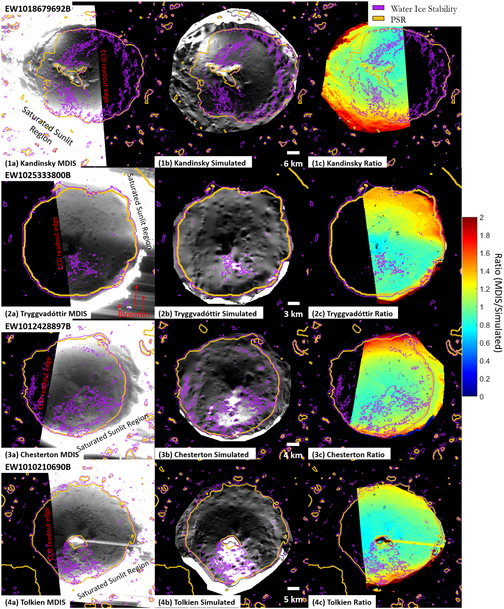
MESSENGER's MDIS Wide Angle Camera (WAC) captured images that revealed the permanently shadowed surfaces within some of Mercury's north polar craters using its broadband filter (Chabot et al. 2014, 2016). These detailed images of the PSRs might allow us to identify boundaries on the volatiles and assess the level of agreement with our models (Figure 2). The WAC broadband filter was designed to obtain calibration images of stars, making it very sensitive to light, with a central wavelength of ∼700 nm and a bandpass of ∼600 nm (Denevi et al. 2018). Since the PSRs are only minimally illuminated by light scattered off of nearby sunlit surfaces, the latter were saturated in these images in order to capture and resolve the details of the surface of the PSRs (Figure 6). When pixels of a charged coupled device (CCD; such as the one used for the MDIS WAC detector) saturate, the charge can spill into adjacent pixels in a process known as blooming. Blooming defaced many of the MDIS WAC images that were attempting to capture the surfaces within the PSRs of the northernmost craters, leaving just a few useful images to examine for each crater. An example of blooming can be seen in Figure 6(2a). Importantly, in these images that were successful at revealing the surface within the PSR, the readout edge of the CCD camera was situated along the PSR, which prevented blooming across the crater floor (Chabot et al. 2014). As a result, though, the whole PSRs could not be captured in a single image.

Figure 6. Comparison of the MDIS WAC broadband and simulated images for each crater. Column (a) depicts the MDIS image of each crater. The unique MDIS image identifier is noted in the upper left corner. The saturated sunlit region and CCD readout edge are labeled in each image. Additionally, we highlight features caused by blooming in panel (2a). Column (b) depicts the simulated image that corresponds to the MDIS image in column (a). Column (c) depicts the ratio between the MDIS and simulated image according to the color bar on the right. The yellow lines in each image outline the PSR of each crater, and the purple lines outline the region where water ice is predicted to be thermally stable at the surface.
Download figure:
Standard image High-resolution imageThe nature of MESSENGER's orbit proved to be simultaneously favorable and detrimental to collecting images to reveal the PSR within Mercury's northernmost craters. MESSENGER's high-eccentricity orbit (Solomon & Anderson 2018) permitted a close-up view of the northern region not obtained for the southern region, which allowed MDIS to acquire high-resolution images of the surface. However, MESSENGER's off-polar inclination diminished the amount of time it spent over the highest-latitude craters, reducing the total number of images ultimately obtained compared to the lower-latitude northern regions. Additionally, near Mercury's pole, the Sun's incidence angle is very near 90°, resulting in a terrain that is heavily shadowed with limited sunlit surfaces to illuminate the PSRs in comparison to lower-latitude locations.
Details of the MDIS WAC broadband images that best revealed the PSR for the four northernmost craters are given in Table 1. Figure 6 shows four of the MDIS images used in this study that best reveal the PSR for each crater in our study, with additional images from Table 1 available in the Appendix. On Figure 6, the yellow lines outline the PSR in each crater, determined by the white region shown in Figure 1(b), while the purple lines outline the region where ice is predicted to be stable at the surface, as described by the white region shown in Figure 1(f).
To aid in examining the MDIS WAC broadband images for evidence of surface volatiles, simulated images were constructed, with the methods from Mazarico et al. (2018) and as used in Hamill et al. (2020). These simulated images were made using the high-resolution DEMs for each crater and the illumination conditions corresponding to the MDIS images in Table 1. Simulated images were produced to predict the radiance (W m−2 sr−1 μm−1) at each imaging time. In these images, a uniform surface albedo is assumed for each crater, allowing us to see how brightness variations emerge from light scattering in the crater owing solely to illumination geometry and topography. This allows us to compare these models to the actual MDIS WAC images and identify inconsistencies in brightness that can only be explained by deviations in surface reflectance, such as those due to the presence of surface volatiles. Figure 6 shows the simulated images and their corresponding MDIS images.
We employed a quantitative approach in our analysis of the MDIS images by finding the ratio of the MDIS images to their corresponding simulated images. With the MDIS images corrected to digital numbers (DN) as described in Hamill et al. (2020) and the simulated images in units of radiance, we first scaled the pixel values of the simulated image to match the values of the MDIS image to achieve a meaningful ratio. We did this by spatially mapping pixels in the MDIS image to the pixels in the simulated image, then with the simulated pixel values on the x-axis and the MDIS pixel values on the y-axis, we found a linear equation for the line of best fit to describe the pixel scaling. Pixels in the MDIS image that were at or near saturation were preemptively removed from the equation calculation in an effort to exclude compromised data. We did this by first excluding saturated pixels and then excluding pixels that were brighter than the mean pixel value. We applied the equation for the line of best fit to the simulated image and then took the ratio between the original MDIS image and the rescaled simulated image. Figure 6 (column (c)) shows the resulting ratio images from this approach. With these ratio maps, we could evaluate how much brighter or darker regions of the MDIS image are compared to regions of the simulated image. In case of a perfect representation, values >1 in the ratio image could be attributed to the presence of surface ice, blooming, or artifacts of the MDIS WAC, while values <1 would hint at low-reflectance volatiles at the surface.
All of the craters in this study have PSRs that cover nearly the entire crater floor, and most are predicted to have ice at the surface in a region that largely overlaps with the PSR. This leaves only a small region for low-reflectance volatiles at the surface, making boundaries between low- and high-reflectance volatiles more challenging to identify. Kandinsky is a special case whose geographic location and topography may allow for a large region of low-reflectance, organic-rich volatile compounds, represented by coronene, to be adjacent to a nearly equally large region of high-reflectance water ice, as shown in Figure 2. However, in these ratio images, we were unable to find conclusive evidence for the presence of high-reflectance volatiles that border low-reflectance volatiles at the surface. We do not observe a significant contrast in brightness along the purple outline in the MDIS images, nor the ratio in Figure 6 for any of the craters, though most notably at Kandinsky, where we would expect this contrast to be most evident.
It is worth noting that in each of the ratio images the ratio tends to be greater along the crater walls than in the center of the images. This brightening effect is likely due to artifacts of the MDIS camera that have been identified as being due to scattered light within the imaging system (Denevi et al. 2018), rather than the presence of exposed, high-reflectance compounds. This phenomenon is more pronounced in the direction that corresponds to the orientation of the readout edge of the CCD (while the readout edge is on the left, we observe a stronger gradient toward the top of the image). This trend of a brightness gradient that is consistent with an MDIS artifact becomes more apparent during these extremely challenging low-light PSR imaging opportunities. So while this feature can be seen in all four images in Figure 6, in Tryggvadóttir (Figures 6(2a) and 11(1a)), it is uniquely abrupt at about midway along the crater and is clearly visible directly in the MDIS WAC broadband image. This feature does not appear to be a consequence of blooming since there are no saturated pixels to the left that could compromise the image. Multiple MDIS imaging orientations would have helped to evaluate if the brightness variation seen within the MDIS WAC broadband images of Figures 6(2a) and 11(1a) of the PSR of Tryggvadóttir is real or rather an anomaly caused by the MDIS camera. However, due to the limited MESSENGER data for Tryggvadóttir, such data are not available.
Our analysis of the other viable MDIS images we identified for each crater (listed in Table 1) showed similar results, which are presented in the Appendix (see Appendix A.2). Our analysis of the MDIS images does not rule out the presence of volatiles on the surface, but rather just shows that there are no obvious features in the available MDIS images that can solely be attributed to the presence of surface volatiles.
3.3. MLA Analysis
MESSENGER's MLA measured the surface albedo at 1064 nm in the northern hemisphere of Mercury (Neumann et al. 2013; Deutsch et al. 2018). At this wavelength, the average reflectance of Mercury's surface is 0.17 (Chabot et al. 2018a). Exposed surface ice on Mercury is observed to be nearly a factor of 2 brighter, with a surface reflectance rs ≥ 0.3 (Deutsch et al. 2017), while low-reflectance volatile materials are observed to be nearly a factor of 2 darker (rs < 0.1; Chabot et al. 2018a).
We used the MLA data (Deutsch et al. 2017) to analyze the brightness variations between the regions where we anticipate ice and low-reflectance volatile compounds, represented by coronene, to be stable at the surface according to the thermal model prediction shown in Figure 2. Barker et al. (2022) found that MLA values that were captured at pulse widths <15 ns, ranges <100 m and >800 m, and emission angles >20° were anomalous or unreliable. We filtered the MLA data according to the pulse width and range constraints identified by Barker et al. (2022). However, due to the lack of data at latitudes >86°N, we chose to remove MLA points at emission angles >35° rather than 20° to retain some MLA data in the northernmost craters of this study for analysis.
All the MLA data between 825 and 90°N latitude with the specified MLA constraints applied are plotted in Figure 7. As is evident from this figure, the data are increasingly sparse with increasing latitude. Additionally, suspect MLA data, especially those due to high emission angles, were abundant at high latitudes where the craters of this study reside, further reducing the already limited data available to reliably examine the craters.

Figure 7. MLA data at pulse widths >15 ns, ranges >100 m and <800 m, and emission angles <35° between 825 and 90°N latitude. The color bar to the right indicates the reflectance value measured at 1064 nm. High-reflectance material is observed to have an rs
≥ 0.3 and would appear red in this figure, whereas low-reflectance volatile material is observed to have an rs
< 0.1 and would appear dark blue in this figure. Note the decrease in density of points with increasing latitude. The northernmost craters examined in this study are labeled.
Download figure:
Standard image High-resolution imageWe plotted the MLA data within the PSR of each of the northernmost craters in Figure 8, where the pink outline represents the region where we predict ice to be stable at the surface. The overall lack of data in these four northernmost craters is apparent in Figure 8. The number of filtered MLA points in the PSR of each crater is given in Table 2. The sum total of MLA points in the four northernmost craters is 485. By comparison, the total number of points in Figure 7 is on the order of 106.

Figure 8. MLA data in the PSR of each crater mapped over the MDIS images from Figure 6. The pink outline represents the region where ice is predicted to be stable at the surface according to the thermal model prediction (Figure 2). The circles (50 m) represent the MLA data and are colored according to their reflectance value as indicated by the color bar on the right.
Download figure:
Standard image High-resolution imageTable 2. Number of MLA Data Points by Crater and Regions Where Volatiles Are Predicted to Be Stable at the Surface
| Crater | Ice Region | Coronene Region | Total |
|---|---|---|---|
| Kandinsky | 244 | 71 | 315 |
| Tolkien | 70 | 2 | 72 |
| Chesterton | 70 | 3 | 73 |
| Tryggvadóttir | 25 | 0 | 25 |
| Total | 409 | 76 | 485 |
Download table as: ASCIITypeset image
While we do not observe a correlation between pixel values in the background MDIS images and MLA reflectance in Figure 8, the MDIS images are not calibrated to reflectance values and, as described in Section 3.2, the extreme low-light conditions make it difficult to image the surface within the PSRs. In looking at the MLA data in Figure 8, we notice that most of the MLA points within the pink outline are very bright (rs > 0.3), consistent with ice being present at the surface, in agreement with our prediction (Figure 2). The MLA data within the region where we predict water ice to be unstable within Kandinsky's PSR do visually appear to be lower reflectance on average (despite the apparent uniformity in the MDIS image), though the number of points in this region, and in comparable regions within the other three craters, is inadequate to determine whether low-reflectance compounds are exposed at the surface.
Figure 9 shows the probability density as a function of the MLA reflectance values for various regions. The purple curve shows the distribution of all of the refined MLA data available between 55° and 90°N latitude. This curve peaks sharply just before 0.2. This is consistent with the average reflectance of Mercury, which we find to be 0.19 with the constrained MLA data set. While the purple curve includes PSRs, the PSRs make up <1% of Mercury's surface between 55° and 90°N latitude, so this curve largely represents the reflectance of Mercury's regolith. By comparison, the yellow curve is the distribution of MLA points in the sunlit region at high latitudes (86°–90°N latitude), which also represents Mercury's regolith, since we anticipate the sunlit regions to be too warm to sustain ice or other volatiles long-term. The relatively enhanced surface reflectance (rs ≥ 0.3) of the adjacent sunlit areas outside the craters, which can be observed in Figure 7, can potentially be ascribed to the presence of small patches of exposed water ice (Deutsch et al. 2017), but the fact that the purple and yellow curves differ substantially, even though both should represent Mercury's regolith, is indicating that care must be taken in interpreting MLA reflectance data acquired at these high latitudes on Mercury owing to the high emission angles prevalent there (Neumann et al. 2013; Deutsch et al. 2017).

Figure 9. Probability density as a function of MLA reflectance. The purple curve represents the distribution of MLA values in the filtered data between 55° and 90°N latitude. This curve largely represents Mercury's regolith since only a small fraction (<1%) of the surface consists of PSRs. The yellow curve represents the distribution of MLA data in the sunlit region surrounding the northernmost craters (86°–90°N latitude). The green curve represents the distribution of MLA in the PSR of the craters, with the red and blue curves representing the MLA distributions of the predicted ice and coronene regions inside the PSR, respectively. Error bars are Poisson errors.
Download figure:
Standard image High-resolution imageIn Figure 9, the green curve is the distribution of MLA points inside the PSR of the northernmost craters. Though subsets of the same purple curve, the green curve entirely excludes sunlit regions, while the yellow curve entirely excludes PSRs in the same latitude range as the green curve. Therefore, comparing the green and yellow curves enables comparison between the MLA data in the PSR, where we expect volatile compounds to be present at the surface, and the MLA data in the surrounding sunlit region, where we do not expect volatile compounds to be at the surface (with the exception of the potential for small patches), with similarly high emission angles.
We find that the PSR of the craters as a whole was found to be brighter than the sunlit region at similar latitudes by a factor of 1.65; this contrast is consistent with an abundance of high-reflectance material at the surface of the PSR rather than artificial brightening caused by the high emission angles in these regions. This result is consistent with the conclusion reached by Deutsch et al. (2017) that demonstrated evidence for high-reflectance surfaces within these four large northernmost craters.
In Figure 9, we also show the results of separating the limited MLA points into regions where ice is predicted to be stable at the surface (red curve) and regions where coronene is predicted to be stable at the surface (blue curve). Unfortunately, the green, red, and blue curves largely overlap, indicating that these regions are statistically indistinguishable owing to the highly limited number of points in the regions where low-reflectance volatiles represented by coronene are predicted to be stable at the surface.
As seen in Figure 8, the points inside the PSR of each crater are primarily contained inside the region where ice is predicted to be stable at the surface, and the blue curve has large error bars and spread, which is consistent with the overall lack of data in the coronene region. In fact, there are only 76 MLA points available for the regions where low-reflectance volatiles like coronene are predicted to be present on the surface, compared to 409 MLA points for the regions where water ice is predicted to be present on the surface as outlined in Table 2. Thus, available MLA data are insufficient to fully test our prediction of precisely where ice or low-reflectance volatiles might be present at the surface within these craters.
4. Summary and Implications
Higher-resolution DEMs (125 m pixel−1) were generated using Shape-from-Shading techniques on the MDIS images obtained by MESSENGER in combination with MESSENGER's MLA data. Following the construction of the DEMs for Kandinsky, Tolkien, Chesterton, and Tryggvaddóttir, we generated illumination and thermal models that support the stability of water ice at the surface within the PSRs of each of these four craters. They also enabled us to predict the stability boundaries of water ice, as well as low-reflectance, complex, organic volatile compounds (represented by coronene in our models) at the surface within these craters.
We found that areas of high radar backscatter are well correlated with areas predicted to host surface and shallow subsurface ice in these four craters. We also identified a class of intermediate radar backscatter intensity within these four craters that occurs near areas of high radar backscatter. Although the thermal environment from these areas would allow surface ice, the much lower radar return suggests significant attenuation or substantially lower abundance of water ice in these regions. This is consistent with heterogeneities within the volatile deposits of Mercury's northernmost craters that are not associated with the thermal environment. These differences may be due to ice purity, mantling of the ice, or uneven ice abundances. As such, this intermediate class of radar backscatter may be the most relevant analog for ice within some lunar PSRs, where impact gardening may have over time efficiently mixed ice with dry regolith (Mitchell et al. 2018; Cannon & Britt 2020).
We examined MESSENGER MDIS and MLA data to search for evidence of water ice and low-reflectance volatiles at the surface within these craters and to evaluate the consistency with our thermal models. We did not find irrefutable evidence for ice or other volatiles at the surface in any of the MDIS images. Our MLA analysis is consistent with previous findings that indicate high-reflectance values present at the surface of these craters (Deutsch et al. 2017), as expected for the presence of water ice at the surface. The limited MLA data >86°N latitude did not enable areas with predicted high-reflectance surface water ice stability and low-reflectance, organic-rich volatile compounds to be distinguished. However, BepiColombo offers an excellent opportunity to revisit these high-interest craters in its upcoming orbital exploration of Mercury, beginning in 2025.
Equipped with the BepiColombo Laser Altimeter (BELA; Thomas et al. 2007, 2021), BepiColombo's Mercury Planetary Orbiter (MPO) will be able to collect laser altimeter data at the same wavelength as MLA. While MESSENGER's orbit had an inclination as low as 825 during its orbital operations (Solomon & Anderson 2018), which limited the observations of the region near Mercury's north pole, BepiColombo's current plans include a polar orbit for MPO that may allow more measurements of Mercury's northernmost craters (Benkhoff et al. 2021). Additionally, MPO is expected to have orbital altitudes ranging from 480 to 1500 km (Benkhoff et al. 2021), compared to the approximately 200–15,000 km orbit of MESSENGER (Solomon & Anderson 2018). Though MPO will be slightly farther than MESSENGER from the northern surface, it will have a less eccentric orbit and a faster orbital period. This may allow the spacecraft to acquire more laser altimeter measurements, particularly in the northernmost craters, in 1 yr than MESSENGER acquired each year of its operations without resulting in a drastic decline in the resolution of data captured in the north. A higher density of altimetry and reflectance data at high latitudes has the capacity to further improve models of the northernmost craters and help to better constrain the water ice and low-reflectance volatiles at the surface.
Additionally, the Spectrometers and Imagers for MPO BepiColombo Integrated Observatory System (SIMBIO-SYS; Flamini et al. 2010; Cremonese et al. 2020) may be able to capture images of permanently shadowed surfaces on Mercury in a similar manner to that accomplished by MDIS, though such imaging by scattered illumination is challenging. Such images could provide a chance to examine the northernmost craters for surface volatiles and to potentially map both high- and low-reflectance materials. In particular, as an imager with distinctly different design and properties than MDIS, a comparison of SIMBIO-SYS and MDIS images of the same crater could offer the opportunity to better distinguish camera artifacts from real features within the PSRs of these four craters. Furthermore, BepiColombo will acquire the first thermal spectral measurements of Mercury with the Mercury Radiometer and Thermal Imaging Spectrometer (MERTIS; Hiesinger et al. 2010, 2020). This instrument may be able to obtain measurements of the mineralogical composition of Mercury's deposits and help us better understand the low-reflectance material that we have modeled as coronene in this study. The results and predictions from this study provide compelling motivation for new measurements of Mercury's northernmost craters during BepiColombo's upcoming mission to further advance the investigation of the distribution of surface ice and volatile compounds on the innermost planet.
Acknowledgments
Support was provided by the NASA Discovery Data Analysis Program grant 80NSSC19K0881 to N.L.C. S.B. acknowledges support by NASA under award No. 80GSFC21M0002. This research made use of the Integrated Software for Imagers and Spectrometers of the U.S. Geological Survey. MDIS and MLA data used in this study are archived at the NASA Planetary Data System. This work made use of data from the NASA-funded Arecibo Observatory planetary radar project. The authors have no conflicts of interest to declare. The data products produced in this study and used to create the figures in this manuscript are available at the JHU-APL Data Archive: https://lib.jhuapl.edu/, specifically at https://lib.jhuapl.edu/papers/investigating-the-stability-and-distribution-of-su/. We express our appreciation for the reviewers whose comments helped to improve this manuscript.
Appendix:
A.1. DEM Data
Table 3 provides a listing of the MDIS images used to create the DEMs for each crater in this study.
Table 3. Catalog of MDIS WAC Images Used to Produce the DEM for Each Crater
| Image | Resolution (m pixel−1) |
|---|---|
| Kandinsky | |
| EW0224424682G | 144.458 |
| EW0246676609G | 174.220 |
| EW0250939615G | 70.797 |
| EW0254280826G | 208.415 |
| EW0254482487G | 178.072 |
| EW0254511306G | 101.533 |
| EW0254540086G | 179.739 |
| EW0254655331G | 178.684 |
| EW0255519506I | 167.814 |
| EW0255548338G | 166.820 |
| EW0255663547G | 172.390 |
| EW0255663560I | 170.480 |
| EW0265572166G | 88.754 |
| EW0265888857G | 222.981 |
| EW1000215185G | 88.452 |
| Chesterton, Tolkien, and Tryggvadóttir | |
| EW0244314682G | 68.710 |
| EW0248865870G | 148.064 |
| EW0248923490G | 145.820 |
| EW0257967850G | 84.988 |
| EW0258054258G | 85.077 |
| EW0258486292G | 84.606 |
| EW0258601500G | 84.497 |
| EW0258803118G | 84.266 |
| EW0258975932G | 83.825 |
| EW0259206354G | 83.416 |
| EW0259580794G | 83.310 |
| EW0259753612G | 83.320 |
| EW0259984039G | 83.645 |
| EW0262000395G | 99.289 |
| EW0262029200G | 99.312 |
| EW0262144418G | 98.957 |
| EW0262230847G | 97.662 |
| EW0263642336G | 91.756 |
| EW0263987991G | 88.898 |
| EW0264247224G | 87.992 |
| EW0264909697G | 88.150 |
| EW0265428154G | 88.489 |
| EW1002317921G | 90.471 |
A.2. Additional MDIS Image Analysis
In addition to the MDIS images shown in Figure 6, we show the other MDIS images that were assessed in this study. Some of the MDIS images presented in this section were more affected by blooming than the ones presenting in Figure 6. While blooming can deteriorate the image quality, we present the images that provide a sufficiently detailed view of the PSR. Only the fraction of images presented in this section, of the more than 50 images that were available for each crater with resolutions better than 200 m pixel−1, were adequate enough for analysis. This is because imaging regions in permanent shadow in an orientation that best prevents blooming is challenging.
Figures 10–13 show the comparison between the MDIS and simulated images for Kandinsky, Tryggvaddóttir, Chesterton, and Tolkein, respectively. The details of the MDIS images can be found in Table 1.

Figure 10. Comparison of the remaining high-quality MDIS WAC broadband and simulated images for Kandinsky. Column (a) depicts the MDIS image, where the unique MDIS image identifier is noted in the upper left corner. Column (b) depicts the simulated image that corresponds to the MDIS image in column (a). Column (c) depicts the ratio between the MDIS and simulated image. The yellow lines in each image outline the PSR of each crater, and the purple lines outline the region where water ice is predicted to be thermally stable at the surface.
Download figure:
Standard image High-resolution image
Figure 11. Comparison of the remaining high-quality MDIS WAC broadband and simulated images for Tryggvadóttir. Column (a) depicts the MDIS image, where the unique MDIS image identifier is noted in the upper left corner. Column (b) depicts the simulated image that corresponds to the MDIS image in column (a). Column (c) depicts the ratio between the MDIS and simulated image. The yellow lines in each image outline the PSR of each crater, and the purple lines outline the region where water ice is predicted to be thermally stable at the surface.
Download figure:
Standard image High-resolution image
Download figure:
Standard image High-resolution image
Figure 12. Comparison of the remaining high-quality MDIS WAC broadband and simulated images for Chesterton. Column (a) depicts the MDIS image, where the unique MDIS image identifier is noted in the upper left corner. Column (b) depicts the simulated image that corresponds to the MDIS image in column (a). Column (c) depicts the ratio between the MDIS and simulated image. The yellow lines in each image outline the PSR of each crater, and the purple lines outline the region where water ice is predicted to be thermally stable at the surface.
Download figure:
Standard image High-resolution image
Figure 13. Comparison of the remaining high-quality MDIS WAC broadband and simulated images for Tolkien. Column (a) depicts the MDIS image, where the unique MDIS image identifier is noted in the upper left corner. Column (b) depicts the simulated image that corresponds to the MDIS image in column (a). Column (c) depicts the ratio between the MDIS and simulated image. The yellow lines in each image outline the PSR of each crater, and the purple lines outline the region where water ice is predicted to be thermally stable at the surface.
Download figure:
Standard image High-resolution image
Figure 10 depicts the comparison of the remaining high-resolution MDIS images that sufficiently detail the PSR of Kandinsky to the corresponding simulated images. In these ratios (Figures 10(1c) and (2c)), we see similar results to Figure 6(1c), in that the brightness appears to increase along the crater walls, likely due to the proximity to the saturated sunlit surface, and that no contrast in brightness that would indicate variations in surface composition is observed, particularly along the purple outline, where we expect to see such variations.
Figure 11 depicts the comparison of the remaining high-resolution MDIS images that sufficiently detail the PSR of Tryggvadóttir to the corresponding simulated images. Much like in Figure 6(2c), Figure 11(1c) depicts an abrupt shift in brightness midway through the crater. While this same shift is not observed in Figure 11(2c), this MDIS image is severely compromised by blooming. Since there are only two images with very similar views of Tryggvadóttir that clearly show this shift in brightness, we cannot make definitive claims about the nature of this feature, and so we look to BepiColombo to investigate further.
Figure 12 depicts the comparison of the remaining high-resolution MDIS images that sufficiently detail the PSR of Chesterton to the corresponding simulated images. In these ratio images (Figures 6(3c) and 12(1–8c)), we observe minor differences. However, we were not able to identify features that could indicate the presence of water ice at the surface in any of them.
Finally, Figure 13 depicts the comparison of the remaining high-resolution MDIS images that sufficiently detail the PSR of Tolkien to the corresponding simulated images. Figures 12(1c) and (2c) show similar results to Figure 6(4c), with little evidence for variations that agree with the prediction (Figure 2).