


Abstract
An internally generated magnetic field once existed on the Moon. This field reached high intensities (∼10–100 μT, perhaps intermittently) from ∼4.3 to 3.6 Gyr ago and then weakened to ≲5 μT before dissipating by ∼1.9–0.8 Gyr ago. While the Moon's metallic core could have generated a magnetic field via a dynamo powered by vigorous convection, models of a core dynamo often fail to explain the observed characteristics of the lunar magnetic field. In particular, the core alone may not contain sufficient thermal, chemical, or radiogenic energy to sustain the high-intensity fields for >100 Myr. A recent study by Scheinberg et al. suggested that a dynamo hosted in electrically conductive, molten silicates in a basal magma ocean (BMO) may have produced a strong early field. However, that study did not fully explore the BMO's coupled evolution with the core. Here we show that a coupled BMO–core dynamo driven primarily by inner core growth can explain the timing and staged decline of the lunar magnetic field. We compute the thermochemical evolution of the lunar core with a 1D parameterized model tied to extant simulations of mantle evolution and BMO solidification. Our models are most sensitive to four parameters: the abundances of sulfur and potassium in the core, the core's thermal conductivity, and the present-day heat flow across the core–mantle boundary. Our models best match the Moon's magnetic history if the bulk core contains ∼6.5–8.5 wt% sulfur, in agreement with seismic structure models.
Export citation and abstract BibTeX RIS

Original content from this work may be used under the terms of the Creative Commons Attribution 4.0 licence. Any further distribution of this work must maintain attribution to the author(s) and the title of the work, journal citation and DOI.
1. Introduction
Paleomagnetic analyses of lunar meteorites and Apollo samples suggest that a high-intensity magnetic field of ∼10–100 μT existed ∼4.25–3.56 billion yr (Gyr) ago, followed by a weakened field of ≲5 μT that persisted until ∼1.9–0.8 Gyr ago (e.g., Tikoo et al. 2014, 2017; Mighani et al. 2020; Strauss et al. 2021; Wieczorek et al. 2022). Generation of an intrinsic magnetic field via dynamo action requires vigorous motion of an electrically conducting fluid, such as the liquid portion of a metallic core (e.g., Bullard 1949; Elsasser 1950; Bullen 1954; Glatzmaier & Roberts 1995; Kageyama et al. 1995). Various observations indicate that the Moon has a metallic core, including seismic data from the Apollo missions (e.g., Garcia et al. 2011; Weber et al. 2011), electromagnetic sounding (e.g., Hood et al. 1999; Shimizu et al. 2013), and gravity data from the Gravity Recovery and Interior Laboratory mission (e.g., Williams et al. 2014), which are all consistent with a core radius of ∼250–430 km. Today, a solid inner core with a radius up to ∼250 km may also exist (Weber et al. 2011; Williams et al. 2014).
Models of the thermal evolution of the lunar core have difficulty reproducing the history of the lunar magnetic field (e.g., Laneuville et al. 2014; Scheinberg et al. 2015; Evans et al. 2018). These models have two goals that often seem incompatible: (1) sustaining a long-lived field (e.g., multiple gigayears) and (2) sustaining an early strong field (i.e., >10 μT, at least for the first ∼1 Gyr). With available energy sources internal to the core (e.g., radiogenic, latent, and chemical energy, plus inner core precession), the Moon can sustain a low-intensity field for long durations (e.g., Laneuville et al. 2014; Scheinberg et al. 2015; Evans et al. 2018; Stys & Dumberry 2020). However, Evans et al. (2018) showed that those energy sources could only sustain a >10 μT field for <50 Myr, assuming that the radius of the core is ≤380 km, as favored by Weber et al. (2011) and Williams et al. (2014). So, sustaining a >10 μT field for ∼1 Gyr is highly improbable without an external mechanism, such as mechanical stirring between the solid mantle and liquid core from precession of the lunar spin axis (e.g., Dwyer et al. 2011; Meyer & Wisdom 2011; Ćuk et al. 2019) and/or impact-induced changes in the rotation rate of the solid mantle (e.g., Le Bars et al. 2011). Another solution to this seeming paradox is to invoke intermittency during the high-intensity epoch. For example, a recent study proposed that foundering of relatively cold material in the lunar mantle may have excited episodes of rapid core cooling that lasted <1 Myr (Evans & Tikoo 2022). Finally, in this study, we explore the idea that the core is not the only potential host for a lunar dynamo, as argued by Scheinberg et al. (2018).
1.1. A Basal Magma Ocean
Almost any scenario for the formation of the Moon involves enough energy to melt much of the newly formed Moon (e.g., Hartmann & Davis 1975; Warren 1985; Elkins-Tanton et al. 2011; Canup 2012; Ćuk & Stewart 2012; Nakajima & Stevenson 2014). The resulting magma ocean is often modeled as solidifying in three primary stages (e.g., Elardo et al. 2011; Wieczorek et al. 2006; Hess & Parmentier 1995; Hamid & O'Rourke 2022). As the lunar magma ocean cooled, dense mafic cumulates (e.g., olivine and pyroxene) formed and sank toward the bottom. Once most of the lunar magma ocean solidified, anorthositic plagioclase with lower density began to crystallize, rising to form the lunar crust. The final, highly evolved liquids, "ur-KREEP" (enriched in uranium, thorium, potassium, rare earth elements, and phosphorus), alongside ilmenite-rich cumulates, would be gravitationally unstable because of their high densities. Some fraction of this ur-KREEP–ilmenite mixture eventually sank to the base of the mantle, ponding as a layer above the core–mantle boundary (CMB). Radiogenic heat from elements present in this fallen ur-KREEP layer, such as uranium, thorium, and potassium (with concentrations up to ∼12 times higher than the bulk mantle), could fully melt this layer (e.g., Scheinberg et al. 2018). The result is a basal magma ocean (BMO) that persists until convective heat loss into the overlying mantle causes solidification. The nominal model of Scheinberg et al. (2018) had a 301 km peak thickness BMO; less conservative models had BMO thicknesses up to 450 km.
Models are equivocal about the lifetime of a BMO. For example, a small compositional density contrast between the BMO and the overlying mantle could make the BMO short-lived (Stegman et al. 2003). In this scenario, thermal expansion of the BMO can overcome the compositional density contrast between the BMO and the overlying mantle, causing the BMO to buoyantly rise and remix with the mantle. Conversely, the persistence of interstitial fluid trapped within the solidified cumulates could leave the BMO sequestered at the CMB (Elkins-Tanton et al. 2011; Scheinberg et al. 2018). Indeed, interpretations of geophysical (Khan et al. 2014), seismic (Weber et al. 2011), and gravity (Williams et al. 2014) data have indicated that a deep-seated zone of partial melt at the CMB may exist today. This partial melt could be the last remnant of a once-thicker BMO.
The lunar BMO could have sustained a dynamo if it was vigorously convecting and had an electrical conductivity, σ, of several thousand siemens per meter (S m−1) (Scheinberg et al. 2018). Such a BMO dynamo would have an advantage over the core in terms of generating strong crustal fields because it is closer to the surface (e.g., Ziegler & Stegman 2013). Magnetic fields attenuate rapidly with distance, so a magnetic field generated in the BMO would appear stronger at the surface than a magnetic field generated with the same strength in the core (e.g., Scheinberg et al. 2018; Stevenson 1983; Christensen 2010). While sufficiently high conductivity is a challenge for this hypothesis, thermal coupling between the BMO and core can fortunately be explored regardless of this uncertainty.
Our study is built on the whole-Moon models presented in Scheinberg et al. (2018). That study focused on the thermal evolution of the solid mantle and BMO to explain the early, strong (i.e., >10 μT) lunar dynamo. Both the BMO and the core were assumed to be well mixed on the timescales of the overlying solid mantle convection and to have an adiabatic temperature gradient, except during the phase in which the magma ocean increases in temperature. That study further tested the sensitivity of their model to the reference viscosity in the solid mantle, the fraction of the KREEP layer that remained near the surface, and the fraction of radioactive material concentrated in the BMO. At the start of their simulations, the BMO exhibited a rapid increase in heat flow from radiogenic heating, followed by a steady decline to its solidus temperature. A detailed model of the core was not included because the core is relatively small and does not strongly affect the thermal evolution of the BMO and solid mantle. In this study, we do not directly model the BMO-hosted dynamo but rather focus on the core to test if models of lunar evolution that feature a BMO as a boundary condition can explain both the strong, early dynamo and the later dynamo that produced much weaker fields (Figure 1).

Figure 1. We study three stages in the coupled evolution of the lunar BMO and core. (Left) Convection in the BMO with the potential to produce an early, high-intensity dynamo ∼4.25–3.56 Gyr ago, while the core was fully liquid. Dashed arrows indicate that in limited scenarios, thermal convection in the core may have occurred in tandem with the BMO-hosted dynamo. (Middle) Compositional convection in the core produced a late, low-intensity dynamo until ∼1.9–0.8 Gyr ago once the inner core started growing and the BMO began to solidify. (Right) The internal field ceased ∼1 Gyr ago; once the BMO solidified sufficiently, the inner core grew too large, and convection ceased in the liquid outer core.
Download figure:
Standard image High-resolution image2. Methods
2.1. Structure of the Metallic Core
We assume that the lunar core is an iron alloy that starts fully liquid with no chemical or thermal stratification. To build our models, we assume that sulfur is the major light element in the core, given its siderophile behavior and cosmochemical abundance (e.g., Pommier 2018; Cameron 1973). Our models also include trace amounts of potassium as a source of radiogenic heating. Other studies have speculated about the possible roles of other light elements in the lunar core, including carbon (e.g., Dasgupta et al. 2009), silicon (e.g., Berrada et al. 2020), and phosphorous (e.g., Yin et al. 2019). However, the complexities of a core with multiple light elements are beyond the scope of this study.
A 1D parameterized description of the structure of the core is the foundation of our models. As described in Appendix A, we used the hydrostatic equilibrium and equations of state detailed in Khan et al. (2018) to calculate the radial profiles of density, pressure, temperature, and gravitational acceleration within the core. Our fiducial structural model assumes that the core contains 6 wt% sulfur and has a central pressure and temperature of 5.15 GPa and 1800 K, respectively, to match the core parameters described in Scheinberg et al. (2018). The radius of the core is then 350 km, which is also the same as in Scheinberg et al. (2018) and in agreement with available observational constraints. However, Scheinberg et al. (2018) used an average density for the core appropriate to a composition of pure iron, which would increase the total mass of the core by ∼20%. Fortunately, most of the structural parameters that are key to our thermodynamic calculations (e.g., K0, K1, Lρ , and Aρ in Table D1) are not sensitive to the bulk composition of the core. Sulfur is most important to the thermal evolution of the lunar core via its effect on the bulk liquidus. Using a fixed sulfur content to calculate other parameters (e.g., ρ0, P0, and MC ) should only introduce inaccuracies that are smaller than the observational uncertainties.
2.2. Energetics of the Metallic Core
The overlying BMO controls the evolution of the core. In the models of Scheinberg et al. (2018), the BMO is initially set to 1700 K at 4.2 Ga, heats up for ∼200 Myr due to radiogenic heating, and subsequently cools until it reaches the initial temperature when the models are stopped. We start tracking the evolution of the core at the time when the BMO starts cooling again. At that time, we assume the core is fully molten and has an adiabatic temperature gradient throughout. We set the "initial" temperature at the top of the core equal to that at the bottom of the BMO. From the results of Scheinberg et al. (2018), we know the total heat flow across the CMB (QCMB) over time:

Here QB
is the heat flow outward from the BMO into the solid mantle,  is the heat associated with secular cooling, and HBMO is the radiogenic heating in the BMO. In order to model the magnetic history of the Moon until the present day (i.e., after the BMO model has stopped), we further assume that QCMB changes linearly to a specified present-day value, which could be the same or (much) less than the value of QCMB when the BMO solidifies. With the boundary condition provided by the BMO model, we then use a well-established method, developed to study Earth's core (e.g., Labrosse 2015), to model the thermodynamic evolution of the lunar core once it starts cooling again. First, we can calculate the global heat budget of the core:

Here QS represents the secular cooling of the core and is proportional to the core's specific heat. We assume that trace amounts of potassium produce radiogenic heating (QR ). The remaining two terms are only relevant once the inner core nucleates: energy from latent heat (QL ) and gravitational energy from the exclusion of light elements into the outer core (QG ) that are released as the inner core grows.
Given the total heat flow, we solve for the rate of change in the CMB temperature. As shown in Appendix B, most of the terms on the right side of Equation (2) are products of d
TCMB/d
t and a term ( ) that depends only on the thermodynamic properties of the core and its structural parameters. Each of those terms is calculable using polynomial functions. We can thus rearrange Equation (2):

The growth rate of the inner core is directly proportional to d TCMB/d t also (see Appendix B). Because Equation (2) does not include any secular cooling of the inner core, we are implicitly assuming that the inner core is perfectly insulating (i.e., with zero thermal conductivity). We could also model a conductive inner core with infinite thermal conductivity, but the associated heat flow is a minor contribution to the global heat budget if the inner core extends to only <75% of the core radius, as expected at the present day. Technically, Equations (2) and (3) are only valid if the liquid portion of the core is convective and thus maintaining a nearly adiabatic thermal profile. This assumption is not valid at the present day since thermal stratification probably exists, because the core heat flux was likely lower than the heat flux that can be conducted along the adiabat for most of the Moon's evolution (e.g., Laneuville et al. 2014).
Our models use a liquidus for the core that depends on the bulk composition. We adapted Equation (29) from Buono & Walker (2011), in which the Fe–FeS liquidus is fit to a polynomial that is fourth order in both pressure and sulfur content. Our model uses an approximation of the liquidus that is first order in both pressure and sulfur content. Specifically, we estimated the approximate pressure derivative (d TL /d P) based on the difference in the liquidus temperatures at 5.15 GPa at the center of the core versus 4.43 GPa at the CMB for 6 wt% sulfur. We found the approximate compositional derivative (d TL /d c) based on the difference in liquidus temperatures for zero versus 25 wt% sulfur at 5 GPa (Table D1).
2.3. Strength of a Core-hosted Dynamo
Vigorous convection in the core can produce a dynamo through the conversion of kinetic to magnetic energy. In general, there are two types of power sources for convection in the core. First, the buoyancy of light elements released from inner core solidification can drive compositional convection. Second, thermal buoyancy from secular cooling of the core, freezing of the inner core, and/or radiogenic heating can power thermal convection. For thermal convection to occur from secular cooling alone, QCMB must exceed the adiabatic heat flow (QAD), which equals the product of the thermal conductivity of the core and the adiabatic temperature gradient (see Appendix B). Once the inner core nucleates, the critical heat flow above which convection occurs is lowered.
We combined the energy and entropy budgets for the core to calculate the total dissipation available to power a dynamo (e.g., Labrosse 2015):

Here ΦL , ΦG , ΦR , and ΦS are the dissipation terms associated with QL , QG , QR , and QS , respectively. The last term (ΦK ) corresponds to the entropy sink associated with thermal conduction in the core. Appendix B contains the polynomial expressions for each dissipation term, which, like the energy terms, depend on the thermophysical properties of the core and its overall cooling rate. Critically, we assume a dynamo exists if the dissipation is positive (i.e., if ΦCMB > 0 W). This criterion yields similar predictions as another often-used criterion, which is that the magnetic Reynolds number (defined below) exceeds a critical value of 50–100 (e.g., Roberts 2007).
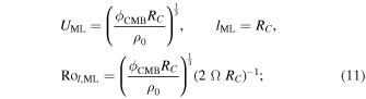
Several scaling laws are available to convert the dissipation (in Watts) into the strength of the magnetic field at the equatorial surface of the Moon (in Teslas). First, we use a scaling law based on core energetics (see Appendix B) to calculate the total dipole moment (DM) of the Moon (units of A m2). In this case, assuming the lunar magnetic field is dipolar, the surface field strength at the magnetic equator is

where RM is the radius of the Moon, and μ0 is the permeability of free space. Additionally, we estimate the magnetic field intensity using three scaling laws that relate the associated convective power to the anticipated convective velocities (e.g., Christensen 2010). These scaling laws use different force balances to calculate the strength of the magnetic field in the core (BC ). First, mixing-length (ML) theory assumes a balance between inertial and buoyancy forces,

where c ∼ 0.63 is a constant of proportionality, ρ0 is the central density in the core, and RC is the radius of the core. Second, assuming a balance of Coriolis, inertial, and gravitational (Archimedes; CIA) forces yields

where Ω is the present-day angular velocity of the Moon, which may underestimate the field strength, since the Moon likely rotated faster in the past. Third, the magneto-Archimedes-Coriolis (MAC) scaling assumes a balance between Lorentz, gravitational, and Coriolis forces:

With these three scaling laws, we calculate the surface field strength of the dipole component as

The ratio of the Moon's core radius to the Moon's radius (RM) accounts for the fact that the dipole field at the surface is smaller than the dipole field at the core (Scheinberg et al. 2018). The prefactor of 1/7 assumes an Earth-like power spectrum for the magnetic field and accounts for the fact that not all of the energy in the magnetic field is partitioned into the poloidal components that can reach the surface (e.g., Christensen et al. 2009; Scheinberg et al. 2018). Note that the core field is assumed to diffuse across an electrically insulating mantle in this approach, thus neglecting the contribution of the BMO. Because the BMO is argued to have a relatively large electrical conductivity, our surface field strength calculations may be considered as lower-bound estimates (discussed further in Section 4.3).
2.4. Local Rossby Number
We further assess the dipolarity of the Moon's magnetic field, particularly whether a dipole-dominated or multipolar dynamo may be preferred. Although there are numerous hypotheses for what controls the breakdown of the dipole (e.g., Soderlund & Stanley 2020), we consider here the local Rossby number,

where Ω = 2π/T is the angular velocity of the Moon, T is the rotation period in seconds, l is the characteristic length scale of the flow, and U is the characteristic fluid velocity. This dimensionless parameter measures the relative importance of inertial to Coriolis forces at convective length scales. Numerical models of planetary dynamos indicate that dipole-dominated solutions tend to be found approximately when Rol < 0.1 (i.e., when inertial effects are relatively weak compared to rotation), with multipolar solutions occurring for larger Rol values (e.g., Christensen & Aubert 2006).
In order to estimate this parameter, we assume a characteristic fluid velocity and length scale following scaling law predictions as done for the magnetic field strengths (e.g., Christensen 2010). The ML scaling yields
the CIA scaling yields
and the MAC scaling yields
Here ϕ = ΦCMB/VOC is the volumetric thermodynamically available power over the fluid core. We could also use these velocity scalings to confirm that the magnetic Reynolds number, which relates the Ohmic diffusion timescale to the convective timescale, exceeds the critical value of ∼50 for magnetic field generation to occur (e.g., Roberts 2007). With the definition

a flow velocity faster than ∼0.1–1 mm s−1 produces Rem > 50 if we assume that the length scale is equal to the core radius and the electrical conductivity is σ ∼ 105–106 S m−1 (e.g., Berrada et al. 2020; Pommier et al. 2020).
2.5. Model Parameters
Our model ingests the BMO model outputs from Scheinberg et al. (2018) and calculates the energy and dissipation budgets for the core to determine when the core may host a dynamo (see Table D2). Following the nomenclature of Scheinberg et al. (2018), naming of the BMO models corresponds to the parameters chosen to describe the mantle and the initial solidification of its magma ocean. For example, V19 indicates a reference mantle viscosity of 1019 Pa s, K50 indicates that 50% of the KREEP layer remained trapped near the surface, and p54 indicates that 54% of the internal radiogenic heating occurs in the sunken KREEP material. We focus on the BMO models that generate magnetic fields with lifetimes of <2.9 Gyr for consistency with the paleomagnetic record (e.g., Mighani et al. 2020). We adopt the nominal BMO case, V19K50p54, as the basis for our nominal model of the core, as it assumes moderate yet reasonable values for the mantle parameters. To test the sensitivity of our models to the properties of the core, we scan across four different parameters: the abundances of sulfur and potassium in the core, the thermal conductivity of the core, and the present-day heat flux at the CMB.
As with other planets, the Moon's core is expected to be an alloy of iron and light elements, such as sulfur (e.g., Steenstra et al. 2016). Properties of the FeS system are relatively well known (e.g., Fei et al. 1997, 2000; Chudinovskikh & Boehler 2007; Morard et al. 2007, 2008; Buono & Walker 2011; Chen et al. 2008; Pommier 2018), and concentrations of sulfur in the lunar core are likely <6–8 wt% based on interpretations of seismic data (e.g., Weber et al. 2011) and models of the lunar core (e.g., Scheinberg et al. 2015; Laneuville et al. 2014). We vary the sulfur abundance, [S], in the bulk core from 1 to 9 wt% in increments of 0.5 wt%.
Potassium is a potential heat source in planetary cores and soluble in iron alloys at planetary conditions (Murthy et al. 2003; Lee et al. 2004). However, the potassium content of the lunar core remains uncertain. Based on previous studies (e.g., Laneuville et al. 2014; Scheinberg et al. 2015), we test a lower limit of 0 ppm, which assumes a complete lack of radiogenic heating in the lunar core. Although the lower pressures and temperatures in the lunar interior might lead to lower amounts of potassium in the lunar core (e.g., Steenstra et al. 2018), we use plausible concentrations of potassium in Earth's core as an upper limit (e.g., Hirose et al. 2013). In our models, we assume that potassium is incompatible in the inner core, meaning that the outer core becomes enriched in potassium as the inner core grows. We vary the bulk potassium abundance, [K], from zero to 50 ppm in increments of 25 ppm.
The thermal conductivity, kC , of iron alloys defines the adiabatic heat flux of the core. We assume that the maximum plausible value of kC is ∼50 W m−1 K−1, cited from thermal conductivity experiments on Fe–FeS alloys in the lunar pressure and temperature range (e.g., Pommier 2018). Small amounts of impurities, such as sulfur, can cause a large reduction in the thermal conductivity. We investigate kC and [S] independently in our models to isolate the effects of each parameter, but they are coupled in reality. A minimum value of 10 W m−1 K−1 is selected to represent relatively large impurities of sulfur (e.g., Pommier 2018). Other proposed compositions for the lunar core, such as Fe–Si alloys, have thermal conductivities that are intermediate between these upper and lower bounds (Berrada et al. 2020). Overall, we vary kC from 10 to 50 W m−1 K−1 in increments of 10 W m−1 K−1.
The present-day heat flux at the CMB is highly uncertain and may have been susceptible to higher heat fluxes out of the lower mantle from the enrichment of water and other incompatible elements during solidification of the lunar magma ocean (e.g., Elkins-Tanton & Grove 2011; Khan et al. 2014; Evans et al. 2014; Weiss & Tikoo 2014; Dygert et al. 2017; Greenwood et al. 2018). To monitor how the core's temperature evolves given a certain heat flow, we test a range of values using thermal evolution models as a guide (e.g., Laneuville et al. 2014). After the BMO solidifies, we assume that QCMB decreases linearly from the final BMO simulation output (∼0.90–3.70 GW) to a heat flux value specified at present. We therefore vary the present-day heat flow, QC , from zero to 2 GW in increments of 1 GW. While the lower limit of 0 GW may represent an extreme scenario, we want to explore a full range of modeling possibilities to account for multiple scenarios for the lunar solid mantle. Furthermore, 1D models for small planetary bodies typically indicate that the heat flux varies slightly during most of the core's evolution (e.g., Laneuville et al. 2014). We find that model outputs from simulations with a QCMB equal to the final BMO simulation output are similar to those from models where the QCMB slightly decreases.
Astute readers will realize that our modeling approach makes the cooling rate of the core seem artificially smooth over time after the BMO solidifies. While the BMO exists, we use QCMB from the 3D solid mantle models of Scheinberg et al. (2018), which contain realistic time variability and fluctuations. Once the BMO has presumably solidified, our parameterized model is effectively 1D and uses a simplified approach for QCMB to capture the average field strength and lifetime of the core dynamo. In reality, some smaller-scale temporal variations in QCMB should be expected, and the very last time step is not necessarily representative of the end of the time series.
We ran a total of ∼800 simulations to test the sensitivity of the core model to [S], [K], kC , and QC using BMO model outputs from Scheinberg et al. (2018) as boundary conditions.
3. Results
3.1. Our Nominal Model for the Evolution of the Core
Our nominal values for the core parameters are [S] = 7.5 wt%, [K] = 25 ppm, kC = 40 W m−1 K−1, and QC = 0 GW for the V19K50p54 BMO boundary condition (Table 1). Figure 2 details the outputs of our nominal model for the core coupled to the nominal BMO model (i.e., V19K50p54). The temperature at the CMB begins at ∼1760 K and quickly spikes to ∼1940 K due to radiogenic heating in the BMO (Figure 2(a)). The BMO then begins solidifying as radiogenic heating declines over time, followed by the core cooling in tandem with the BMO. Once the BMO solidifies, an inner core forms at ∼2.2 Gyr as relatively pure iron crystallizes from the inside out (Figure 2(b)), expelling sulfur into the outer core (Figure 2(c)). Our models assume that the lunar core always contains sub-eutectic amounts of sulfur. We verified that this assumption is consistent with our results, which track the sulfur content of the outer core over time (e.g., Figure 2(c)). The liquidus temperature of the outer core is lowered as it is progressively enriched in sulfur. The result is a molten outer core and a growing inner core. The heat flow is always less than that transported by thermal conduction along the core adiabat, QAD. After the inner core nucleates, most extracted heat from the core arises from the release of QG and QL (Figure 2(d)). The release of QG is nonzero but small compared to QL. Following the release of QG and QL , there is a reduction in the core cooling rate due to these heat sources acting as a buffer to secular cooling. We note that the QCMB is much lower than the heat flow across the upper boundary of the BMO (QB = ∼100 GW at 2.6 Ga) in Scheinberg et al. (2018) because QB includes radiogenic heating in the BMO and the heat associated with cooling the BMO itself.
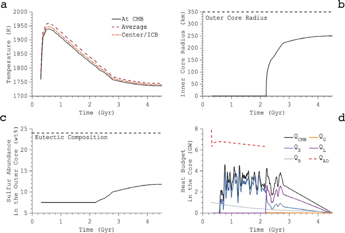
Figure 2. Results of the nominal core model with kc = 40 W m−1 K−1, QC = 0 GW, [S] = 7.5 wt%, and [K] = 25 ppm coupled to the nominal BMO model (V19K50p54). All models began at 4.2 billion yr before the present day. (a) Temperature at the CMB, at the center of the core, or near the inner core boundary (ICB) and the average temperature of the core. (b) Inner core radius with respect to time. (c) Sulfur abundance in the outer core with respect to time. (d) Heat budget given by latent heat, QL ; radiogenic heating, QR ; gravitational energy, QG ; adiabatic heat flow in the core, QAD; heat flow across the CMB, QCMB; and secular cooling, QS .
Download figure:
Standard image High-resolution imageTable 1. Nominal Core Parameters for Each BMO Boundary Condition Used in This Study
| Nominal Core Model Inputs | ||||||
|---|---|---|---|---|---|---|
| BMO boundary condition | V19K50p54 | V19K50p36 | V19K50p27 | V19K25p54 | V18.5K50p54 | V18K00p100 |
| BMO lifetime a (Gyr) | 2.6 | 2.0 | 1.6 | 2.9 | 1.2 | 2.1 |
| BMO thickness (km) | 301 | 301 | 301 | 383 | 301 | 450 |
| [S] (wt%) | 7.5 | 7.0 | 8.5 | 7.0 | 8.5 | 6.5 |
| [K] (ppm) | 25 | 0 | 0 | 50 | 0 | 50 |
| QC (GW) | 0 | 0 | 0 | 0 | 0 | 0 |
| kC (W m−1 K−1) | 40 | 10 | 30 | 40 | 30 | 30 |
Note.
a Values are from Scheinberg et al. (2018).Download table as: ASCIITypeset image
Abundant sulfur influences the core's ability to drive a magnetic field by lowering its solidus temperature and controlling the onset of inner core crystallization (discussed further in Section 3.2.1). The nominal model produces an inner core radius of 250 km at the present day (Figure 2(b)) and is consistent with core radii derived from calculated models of lunar gravity data (Williams et al. 2014) and reanalyzed Apollo seismic data (Weber et al. 2011).
The lunar BMO suppresses convection in the core by lowering its cooling rate. The core produces a dynamo that begins near the cessation of the nominal BMO-hosted dynamo and ends at ∼1 Ga, consistent with the lower estimate on the cessation of the lunar dynamo derived from radiometric dating of Apollo 15 samples (e.g., Mighani et al. 2020; Figure 3(a)). The relatively weak surface magnetic field strength of ≲2.55 μT is also consistent with the paleomagnetic data and intensities from previous models of the lunar core dynamo (e.g., Laneuville et al. 2014; Tikoo et al. 2014, 2017; Evans et al. 2018; Mighani et al. 2020).

Figure 3. (a) Surface field intensities of the nominal core model where core convection is driven by inner core growth relatively late in the Moon's history. The BF, ML, CIA, and MAC scaling laws are used to estimate the surface field intensities of the dipole component. Surface field intensities are compared to the nominal BMO magnetic field intensity assuming the ML scaling law. (b) The dissipation budget of the nominal core model includes the entropy sink associated with thermal conductivity ΦK ; the dissipation associated with secular cooling ΦS , latent heat ΦL , gravitational energy ΦG , and radiogenic heating ΦR ; and the dissipation available for a dynamo ΦCMB. (c) If kC is lowered to 30 W m−1 K−1, purely thermal convection occurs intermittently between ∼0.7 and 2 Gyr. Those resultant surface fields are several times weaker than the BMO-hosted field. (d) Dissipation budget associated with a lower kC of 30 W m−1 K−1.
Download figure:
Standard image High-resolution imageWe next consider different BMO conditions for our core model. Table 1 presents the nominal core input parameters for each BMO boundary condition used in this study. The BMOs with a smaller fraction of KREEP that remained near the surface (i.e., V19K25p54 and V18K00p100 in Table 1) have greater initial thicknesses and tend to require lower sulfur abundances (6.5–7 wt%) in the bulk core to initiate dynamo action during the observed timing of the low-intensity epoch. Because a BMO with a greater thickness will have a longer lifetime (e.g., Scheinberg et al. 2018), the core will begin crystallizing at a later time, when the BMO eventually solidifies. Conversely, models with shallower BMOs (i.e., 301 km) mostly require higher sulfur abundances in the core (7–8.5 wt%) to achieve a core dynamo during the same period. The BMO boundary conditions with greater lifetimes additionally suppress inner core growth for longer periods, resulting in smaller inner core radii at the present day. Furthermore, models that contain shallower BMOs match the estimated timing of the lunar dynamo if balanced by less radiogenic heating in the core (i.e., ≤25 ppm of potassium). In general, BMO boundary conditions typically require the core to have a higher thermal conductivity (i.e., ≥30 W m−1 K−1) to match the estimated timing of the lunar dynamo.
3.2. Sensitivity Tests
3.2.1. Influence of Sulfur in the Core
An inverse relationship exists between the sulfur content and the solidus temperature of the core. As the sulfur content increases, the solidus temperature of the Fe–S system decreases, delaying core solidification until lower temperatures are reached. Therefore, the timing of inner core growth, and thus the start time of compositional convection in our models, depends on the sulfur content of the bulk core (Figure 4(a)). The sulfur concentration is viable when the end of the core-hosted dynamo matches the lower estimate on the cessation of the lunar dynamo at ∼1 Gyr (e.g., Mighani et al. 2020). Initial sulfur abundances of 1–6.5 wt% result in inner core nucleation at higher temperatures, causing the core to solidify rapidly early in its history (Figure 4(b)). Sulfur abundances from 7 to 8.5 wt% result in the inner core nucleating near the cessation of the BMO-hosted dynamo. Increasing the bulk sulfur content to >8.5 wt% further delays inner core growth and generally results in temporal gaps between the BMO- and core-hosted dynamos, a complete lack of core dynamo action, or contradictions with timing estimates derived from paleomagnetic data (Figure 4(c)). However, if the BMO model assumes a lower solid mantle viscosity (i.e., V18.5K50p54), then convective heat transfer is more efficient and results in shorter BMO lifetimes (Scheinberg et al. 2018). As a result, the inner core begins crystallizing earlier, and a bulk sulfur content of up to 12 wt% can produce results consistent with the lower estimate on the cessation of the lunar dynamo (e.g., Mighani et al. 2020). The trends outlined in Figure 4 that arise from variations in kC , [K], [S], and QC continue under all other BMO boundary conditions.

Figure 4. Sensitivities of the nominal core model to core parameters kC , [K], [S], and QC for the nominal V19K50p54 BMO model. (a) The surface magnetic field intensity is most sensitive to kC and [S] and less sensitive to [K] and QC . (b) Our choice of [S] controls the predicted timing of inner core growth and thus a compositionally driven core dynamo. The shaded region represents inner core radii that are probably inconsistent with lunar gravity data (e.g., Williams et al. 2014). (c) The duration of the dynamo is predicted to increase with increasing QC and decreasing kC . High [S] tends to delay the onset of inner core crystallization and result in a shorter field duration. The shaded region represents durations that are likely inconsistent with constraints on the end of the lunar dynamo (e.g., Mighani et al. 2020). The magnetic field intensity and the duration of the core dynamo are given by the MAC scaling law.
Download figure:
Standard image High-resolution image3.3. Influence of the Core's Heat Budget and Thermal Conductivity
The duration and intensity of the core dynamo are also sensitive to kC , QC , and [K] (Figure 4). A potassium abundance of 50 ppm in the core contributes thermal energy to the dynamo but suppresses growth of the inner core, which can decrease the predicted intensity of the magnetic field overall. Decreasing [K] has a minimal effect on the field intensity because radiogenic heating is nearly equivalent to secular cooling in the dissipation budget. In contrast, increasing the total heat flow to 1–2 GW increases the duration and strength of the core-hosted dynamo, unless a low sulfur abundance leads to rapid core solidification. Furthermore, the duration and intensity of the field generally increase with decreasing thermal conductivity values. We find that purely thermal convection typically occurs before the onset of inner core crystallization if the thermal conductivity is low (i.e., 10–30 W m−1 K−1 as in Figure 3(c)). As thermal conductivity decreases, the superadiabatic heat flow increases, leading to a stronger, more long-lived dynamo. Thermal convection–driven dynamos typically occur simultaneously with BMO-hosted dynamos, as the core is still hot and fully molten. Compared to the abundance of sulfur in the bulk core, our simulations reveal that small variations in parameters such as kC , QC , and [K] play an overall negligible role in the onset of a compositionally driven dynamo, whereas a thermal convection–driven dynamo is largely dictated by kC .
3.4. Strength and Timing of the Core Dynamo
Depending on the BMO boundary condition, inner core crystallization can produce fields of ∼0.7–2.3 Gyr in duration, with peak magnetic fields of 0.16, 0.45, 0.77, and 4 μT for the ML, CIA, BF, and MAC scaling laws, respectively (Table 2). A general issue arises in the case of the CIA, ML, and BF scaling laws in which the strengths are not sufficient to reproduce the first period of decline to ∼4–7 μT by 3.19 Ga (e.g., Strauss et al. 2021) or the second period of decline to ∼5 ±2 μT by ∼1–2 Ga (e.g., Tikoo et al. 2017; Mighani et al. 2020). However, intensities ranging from ∼1.7 to 4 μT can be achieved under all BMO boundary conditions if the MAC scaling law is assumed. In particular, an intensity of 4 μT is achieved if the BMO boundary condition contains a lower fraction of radioactive material concentrated in the BMO (i.e., V19K50p36). However, this magnetic field weakens to a maximum of 4 μT ∼2 Gyr after accretion, which is ∼0.7 Gyr later than what is observed in the lunar paleomagnetic record (Strauss et al. 2021).
Table 2. Nominal Core Model Outputs for Each BMO Boundary Condition Used in This Study
| Nominal Core Model Outputs | ||||||
|---|---|---|---|---|---|---|
| BMO boundary condition | V19K50p54 | V19K50p36 | V19K50p27 | V19K25p54 | V18.5K50p54 | V18K00p100 |
| Present-day inner core radius (km) | 250 | 257 | 231 | 226 | 262 | 241 |
| Compositional convection Bmax (μT) | 0.07 (ML) | 0.16 | 0.05 | 0.03 | 0.07 | 0.04 |
| 0.13 (CIA) | 0.45 | 0.09 | 0.04 | 0.13 | 0.08 | |
| 0.36 (BF) | 0.77 | 0.27 | 0.20 | 0.40 | 0.28 | |
| 2.55 (MAC) | 4.0 | 2.27 | 1.7 | 2.6 | 2.0 | |
| Thermal convection Bmax (μT) | 3 × 10⁻⁶ (ML) | 0.001 | 0.002 | 3 × 10⁻⁴ | 0.001 | 0.002 |
| 3 × 10⁻⁷ (CIA) | 3 × 10⁻⁴ | 0.001 | 9.3 × 10⁻⁵ | 2 × 10⁻⁴ | 0.001 | |
| 0.001 (BF) | 0.08 | 0.07 | 0.02 | 0.06 | 0.06 | |
| 0.003 (MAC) | 0.30 | 0.31 | 0.08 | 0.23 | 0.28 | |
| Combined Bmax (μT) | 0.07 (ML) | 0.16 | 0.052 | 0.03 | 0.071 | 0.042 |
| 0.13 (CIA) | 0.45 | 0.091 | 0.04 | 0.13 | 0.081 | |
| 0.36 (BF) | 0.85 | 0.34 | 0.22 | 0.46 | 0.34 | |
| 2.55 (MAC) | 4.3 | 2.58 | 1.78 | 2.83 | 2.28 | |
| Peak local Rossby number | 0.02 (CIA) | 0.03 | 0.02 | 0.02 | 0.02 | 0.03 |
| 0.003 (ML) | 0.004 | 0.003 | 0.003 | 0.003 | 0.003 | |
| 3 × 10⁻⁴ (MAC) | 4 × 10⁻⁴ | 2 × 10⁻⁴ | 2 × 10⁻⁴ | 2 × 10⁻⁴ | 3 × 10⁻⁴ | |
| Compositional convection duration (Gyr) | 1.14 (ML) | 1.83 | 1.90 | 0.66 | 2.23 | 1.42 |
| 1.14 (CIA) | 1.75 | 1.86 | 0.66 | 2.23 | 1.42 | |
| 1.06 (BF) | 1.75 | 1.78 | 0.58 | 2.22 | 1.34 | |
| 1.12 (MAC) | 1.89 | 1.95 | 0.71 | 2.33 | 1.49 | |
| Thermal convection duration (Gyr) | 0.05 (ML) | 0.87 | 0.08 | 0.12 | 0.85 | 1.65 |
| 0.05 (CIA) | 0.87 | 0.08 | 0.12 | 0.85 | 1.65 | |
| 0.05 (BF) | 0.87 | 0.08 | 0.12 | 0.85 | 1.65 | |
| 0.05 (MAC) | 0.87 | 0.08 | 0.12 | 0.85 | 1.65 | |
| Lifetime of core-hosted dynamo (Gyr) | 1.19 (ML) | 2.70 | 1.98 | 0.78 | 3.08 | 3.07 |
| 1.19 (CIA) | 2.62 | 1.94 | 0.78 | 3.08 | 3.07 | |
| 1.11 (BF) | 2.62 | 1.86 | 0.7 | 3.07 | 2.99 | |
| 1.17 (MAC) | 2.76 | 2.03 | 0.83 | 3.18 | 3.14 | |
Note. Compositional and thermal convection in the core sustains low-intensity magnetic fields following the cessation of a BMO-hosted dynamo. Here Bmax is the peak magnetic field intensity at the surface according to the ML, CIA, BF, and MAC magnetic field scaling laws, assuming that the mantle is electrically insulating. The thermal convection Bmax corresponds to the ML, CIA, BF, and MAC scalings. The combined Bmax is the sum of the surface fields generated from thermal and compositional convection. The peak local Rossby number corresponds to the CIA, ML, and MAC scaling laws. The thermal convection duration corresponds to the ML, CIA, BF, and MAC scalings.
Download table as: ASCIITypeset image
Surface magnetic fields are weaker if they are driven by thermal convection rather than inner core crystallization. The peak surface magnetic field driven by thermal convection in the nominal core model is 3 × 10⁻⁶, 3 × 10⁻⁷, 0.001, and 0.003 μT for the ML, CIA, BF, and MAC scaling laws, respectively (Table 2). For all BMO boundary conditions, thermal convection in the core is initiated ∼3.7 Gyr ago (albeit briefly in some models; e.g., Figure 3(a)). Furthermore, depending on the BMO boundary condition, thermal convection can persist intermittently for up to ∼1.7 Gyr, resulting in an overlap with the BMO-hosted field (e.g., Figure 3(a)). Thermal convection produces intensities that are consistent with previous modeled estimates of the core (e.g., Laneuville et al. 2014; Evans et al. 2018; Scheinberg et al. 2015) but inconsistent with paleomagnetic analyses constraining the initial and final decline of the lunar dynamo (e.g., Tikoo et al. 2017; Mighani et al. 2020; Strauss et al. 2021). Furthermore, these results are consistent with a low-intensity epoch that persisted from ∼1.9 to 0.8 Ga (e.g., Mighani et al. 2020; Tikoo et al. 2017, Tikoo et al. 2014; Strauss et al. 2021).
An uneven heat flow across the CMB may make the magnetic field intermittent because dynamos can be sensitive to slight variations in heat flow (Scheinberg et al. 2015). As an artifact of our modeling approach, early magnetic fields produced via thermal convection are discontinuous due to fluctuations in the QCMB from mantle dynamics. In some cases, thermal convection generates fields that are predicted to drop to zero multiple times before rising again from inner core crystallization. The duration of these gaps in the magnetic field is much longer than the magnetic diffusion time (Appendix C). Using the nominal models but with core conductivity lowered to kC = 30 W m−1 K−1 as an example case (i.e., Figure 3(c)), gaps in thermal convection last, on average, ∼140 Myr, whereas the magnetic diffusion time is only a few hundred years. Alternatively, dynamos induced by thermal convection can transition directly into those induced by inner core crystallization, compounding the resultant fields.
3.5. Local Rossby Number
In order to make initial predictions for the magnetic field morphologies in our models, we estimate the local Rossby number as a proxy for whether the core dynamos would be dipole-dominated or multipolar, as has been done for Ganymede's dynamo (Ruckriemen et al. 2015), for example. The CIA scaling law predicts higher values of the local Rossby number (Rol ∼ 10−2) relative to the ML (Rol ∼ 10−3) and MAC (Rol ∼ 10−4) scaling laws, since inertia plays a larger role in the force balance (Christensen & Aubert 2006). However, for the nominal core model, all scaling laws predict that the local Rossby number is below the threshold value of ∼0.1 throughout the lifetime of the core dynamo, suggesting a prevailing dipole-dominated magnetic field (Table 2 and Figure 5).

Figure 5. Predictions of the local Rossby number for the nominal core model estimated from CIA, ML, and MAC scaling laws.
Download figure:
Standard image High-resolution image
4. Discussion
In this study, we demonstrated that a BMO dynamo could naturally dovetail with a core dynamo. Future studies should further explore this hypothesis by addressing the following important issues.
4.1. Other Modes of Crystallization in the Core
Future studies could model more complex modes of crystallization in the lunar core. To recap, we made two relevant assumptions. First, we assumed that the core always contains sub-eutectic amounts of sulfur, which most of our models indeed predict (Section 3.2.1). Second, we assumed that the core solidifies from the center outward. We set the liquidus temperature to increase faster than the adiabatic temperature with pressure (e.g., with gradients of 30 versus ∼23–25 K GPa–1, respectively).
Future studies could relax these two assumptions, which would produce more complicated behavior in models (e.g., Hauck et al. 2006). First, FeS rather than Fe could crystallize from the outer core as it cooled if the sulfur content were supereutectic. Being sulfur-rich compared to the residual liquid, solid FeS would float to the top of the liquid rather than sink to form an inner core like solid Fe. Second, solidification could occur at the top or middle of the outer core, rather than at its bottom. For example, "iron snow" could occur in metallic cores if the liquidus crosses the adiabat above the base of the outer core. This process could help drive a dynamo as the solidified iron sinks and remelts in the warmer fluid below, leading to compositional convection (e.g., Williams 2009; Breuer et al. 2015). Whether the Moon's core entered an FeS crystallization or Fe snow regime at any time remains an ongoing question.
Scientists might make more realistic models of the thermal evolution of sulfur-rich cores if they include these processes. Such models require detailed phase diagrams for the Fe–FeS system. The neglect of Fe snow and FeS crystallization in our models does not change our takeaway message, however, that the presence of a BMO overlying the core may influence the timing and intensity of the core dynamo. Our models may interface with future, more detailed descriptions of Fe snow and FeS in the core.
4.2. Morphology of the Lunar Dynamo
The geometry and paleo-orientation of the Moon's magnetic field remain largely uncertain. Estimates of paleoinclinations from five Apollo samples suggest the existence of a dipolar field and a paleopole located at ∼75°N between 3.8 and 3.3 billion yr ago (e.g., Cournède et al. 2012). These findings are possibly best explained with a paleofield geometry close to the present-day rotation axis of the Moon. Assumptions of the paleopole were made based on the location of the Apollo samples; samples collected from the northern hemisphere were given a positive declination, while samples collected from the southern hemisphere were given a negative declination. However, the sign of the inclination remains largely unknown, and more data are required to confirm interpretations made from lunar samples. Studies of Apollo 17 mare basalts estimated an inclination of ∼34° based on the layering of its parent boulder (Nichols et al. 2021). This inclination is consistent with, but does not require, a dipole in the center of the Moon aligned along its rotation axis.
Conversely, Olson & Christensen (2006) hypothesized that the Moon's magnetic field may have been multipolar rather than dipole-dominated. The critical difference between our studies is the amplitude of buoyancy flux (BF) in the core. Their study assumed that the average BF associated with convection in the lunar core was 0.3 times the terrestrial value. That is, FMoon = 0.3 FEarth, where F = αgQ/(ρ Cp ) with thermal expansivity α, gravitational acceleration g, convective heat flux Q, density ρ, and specific heat capacity Cp . This assumption was based on the idea that tidal dissipation could add several TW of power to the ancient lunar core (e.g., Williams et al. 2001). This larger heat flow leads to larger estimates of the local Rossby number (e.g., Rol ∼ 2), which would shift the lunar dynamo into a multipolar regime. In contrast, our models do not include tidal heating in the lunar core. So the total power available for convection is only several GW in our models, as shown in Figure 2(d).
It is also possible that the directional magnetization of lunar rocks does not record a long-term orientation of the lunar magnetic field, since differential rotations between the mantle and core would cause a core dipole field to drift across the lunar surface (e.g., Ćuk et al. 2019). Relative motions of the core and mantle or misalignment between the lunar dynamo and spin axis may further explain the great variability in the inferred orientation of the lunar dynamo from proposed paleopole locations (e.g., Oliveira & Wieczorek 2017; Nayak et al. 2017). Future missions sampling the lunar bedrock along varying latitudes will allow for more precise geometric determinations of the Moon's magnetic field.
4.3. Electromagnetic Core–Mantle Coupling
The effects of an electrically conducting lower mantle on the core dynamo is not considered in our study. This limitation is significant for several reasons. First, as noted in Section 2.3, the relatively large conductivity of the BMO, especially when it is fully liquid, will likely cause our estimates of surface magnetic field strengths to be artificially small compared to if this conductivity were taken into account. Our estimates for the core field strength assume that the entire mantle, including the BMO, is electrically insulating such that the core-generated magnetic field becomes a potential field that diffuses upward through the mantle. Given the anticipated higher conductivity of metalliferous silicate melts compared to solid mantle rocks (e.g., Scheinberg et al. 2018), the top of the dynamo region may effectively be the top of the BMO, rather than the top of the core, even if the BMO is subcritical for dynamo action.
Second, fluid flows within the BMO may also modulate the core field itself (e.g., Gómez-Pérez et al. 2010). Conversely, if the BMO fluid is stably stratified, its presence may still filter out small-scale components of the core field that rapidly vary via the magnetic skin effect (e.g., Christensen 2006). Third, the BMO may have resulted in a larger magnetic coupling between the core and mantle in the past, relevant to studies of the Moon's rotational dynamics over time (e.g., Dumberry & Wieczorek 2016). Further work, such as numerical dynamo modeling, is needed to better understand the full degree of coupling between the BMO and core of the Moon.
4.4. Thermal Stratification in the Core
The effects of thermal stratification in the lunar core are not considered in this study. The inclusion of thermal stratification can have several effects on the heat flux at the CMB. Studies of Mercury's core (e.g., Knibbe & van Westrenen 2018; Knibbe & Van Hoolst 2021) found that thermal stratification can lead to an increased inner core size, higher temperatures, and a larger heat flux at the CMB, which together result in an early start to the magnetic field. Subsequent heat released upon core solidification would enable slow core growth and an active magnetic field until the present day. Future work could apply these models of Mercury to the Moon.
4.5. The Early Evolution of the Moon
Thermal stratification is probably inevitable at the present day but could also exist early in the Moon's history. In this study, we assume that the core was initially fully molten and had an adiabatic temperature gradient. If radiogenic heating in the BMO ever made the bottom of the BMO hotter than the top of the core, then heat would move from the BMO into the core, which would cause thermal stratification at the top of the core that might delay the start of a core-hosted dynamo. However, the Moon could have formed with "superheat" (such that the core was initially hotter than the BMO; e.g., Evans et al. 2018), in which case the core could deliver heat to the BMO even while the BMO heats up radiologically. Neither our study nor Scheinberg et al. (2018) modeled these two countervailing possibilities in detail. Further work is thus needed to better understand the formation and early evolution of the Moon.
5. Conclusions
Our model for the coupled evolution of a basal magma ocean (BMO) and the core places estimates on the abundance of sulfur in the core (i.e., 6.5–8.5 wt% in Table 1) and can explain the timing and relative intensity of the lunar magnetic field consistent with other models of the lunar core (e.g., Laneuville et al. 2014; Evans et al. 2018; Scheinberg et al. 2015). The BMO does not need to be electrically conductive to explain the results presented here, even if it was required to explain the results of Scheinberg et al. (2018). While that may mean that the early, intense lunar dynamo remains unexplained, we find that the predicted timing of the lunar dynamo in our models is most consistent with observational constraints of the long-lived low-intensity period when moderate abundances of sulfur and potassium are assumed in the core, the core's thermal conductivity is high, and the present-day CMB heat flow is assumed to be low (or even zero). Excessively high values of QCMB at the present day (i.e., 1–2 GW) tend to increase the duration of the magnetic fields longer than is consistent with timing constraints on the end of the lunar dynamo (e.g., Mighani et al. 2020). Modeled intensities are most consistent with paleomagnetic analyses constraining the initial and final decline of the lunar dynamo (e.g., Tikoo et al. 2017; Mighani et al. 2020; Strauss et al. 2021) when the BMO boundary condition is assumed to have less radiogenic heating concentrated in the BMO or the MAC scaling is assumed. Other scaling laws (i.e., CIA, ML, and BF) predict that magnetic field intensities would be ∼1–2 orders of magnitude weaker at the surface than inferred from paleomagnetic data (although recall that our intensities may be higher if electrical conductivity of the BMO is taken into account).
Thermal convection can briefly exist with the BMO but is generally short-lived (Figure 3(a)) or intermittent (Figure 3(c)), generating magnetic field intensities of up to ∼0.3 μT that persist for ≲1.7 Gyr (Table 2). Near the cessation of the lunar BMO dynamo, the heat flows are too low for purely thermal convection, and later dynamo action requires inner core crystallization. Magnetic fields generated from the onset of inner core crystallization can reach intensities of up to ∼4 μT and persist for ≲2.3 Gyr (Table 2). Temporal gaps may arise between dynamos powered by different types of energy in the core (i.e., thermal versus compositional), which are neither confirmed nor excluded by extant data. Temporal gaps in the magnetic field can lead to complications in interpretations of the paleomagnetic record and may indicate that a portion of Apollo samples with null paleointensities (e.g., Tarduno et al. 2021) may not result from poor magnetic recording properties.
Estimates of the core sulfur abundance from our model can further translate into predictions of the radius of the inner core. These predictions can be verified with future missions, such as the Farside Seismic Suite (e.g., Panning et al. 2021), which will provide new constraints on the internal structure of the Moon, and the Lunar Geophysical Network (e.g., Weber et al. 2021), which aims to understand the size, state, and composition of the lunar core and the chemical and physical stratification of the mantle. Together, these findings will help discriminate between hypotheses that seek to explain the high–low intensity epoch. Research on the Moon's magnetic history should remain fruitful for decades.
This material is based upon work supported by the National Science Foundation Graduate Research Fellowship under grant No. 026257-001. We thank Aaron Scheinberg for providing the complete outputs of published simulations.
Appendix A: Radial Structure of the Lunar Core
We approximated the lunar core as a mixture of liquid Fe and liquid Fe-10 wt% S to make structure models. We followed the procedure detailed in Khan et al. (2018), especially their Appendix A, to calculate radial profiles of density, pressure, and temperature. We use the mass-weighted averages of the depth-dependent values of the Grüneisen parameter and the coefficient of thermal expansion. We then performed a least-squares fit to parameterize the radial density using a fourth-degree polynomial,

where ρ0 is the density at the center of the core, Lρ is a length scale, and Aρ is a constant. The effective bulk modulus is then K0 = 2π G(Lρ ρ0)2/3, where G is the gravitational constant. The derivative of the effective bulk modulus is K1 = (10Aρ + 13)/5. Finally, the adiabatic thermal gradient in the core is then Ta (r) = T(0)[ρ(r)/ρ0]γ .
Appendix B: Energetics of a Dynamo in the Lunar Core
Section 2.2 describes the heat budget of the lunar core. For completeness, we list here the polynomial equations used to calculate the different terms. Analogous equations that were developed to model Earth's core can be found in Labrosse (2015), albeit with slightly different notation and additional complexities added to the analytic formulation, and in the Supporting Information for Blaske & O'Rourke (2021).
In our models, the total heat flow across the CMB can be partitioned into four different terms, each of which is proportional to the overall cooling rate of the core (d TCMB/d t). First, we have the heat flow associated with secular cooling of the fluid portion of the core. Before the inner core nucleates, we have

where
After the inner core nucleates,
where TL (RI ) is the liquidus temperature evaluated at the inner core boundary given by

Here c0 is the mass fraction of sulfur in the outer core, which increases as the inner core grows. Differentiating this equation yields the slope of the liquidus at the inner core boundary:

Following Nimmo (2015), we use this slope and the adiabatic thermal gradient to calculate the growth rate of the inner core:

The growth of the inner core also releases latent heat,

where ΔSC = 200 J K–1 kg–1 is the entropy of melting for the inner core (Nimmo 2015). Next, we compute the gravitational energy related to the exclusion of sulfur from the inner core as it freezes,
where αI = 2.3 is the coefficient of compositional expansion for enriching the outer core in sulfur (Nimmo 2015). Here we leverage another useful function:

Last and easiest, the radiogenic heat in the core is

where λK = 1.76 × 10⁻¹⁷ s−1 and HK = 4.2 × 10⁻¹⁴ W kg–1 ppm–1 are the decay constant and heat production rate at t = 0 for potassium-40, respectively.
The energy budget by itself does not reveal whether a dynamo might exist in the lunar core. We must compute the dissipation budgets, again following Labrosse (2015) and studies such as Blaske & O'Rourke (2021). First, we expand Equation (3) in the main text as

Here we use the average temperature in the outer core:
The effective temperature associated with dissipation from secular cooling is almost identical to TD but slightly hotter:

Finally, we can calculate the dissipation sink associated with the thermal conductivity of the core fluid,

where our last useful function is
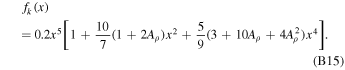
Note that we can then write the total adiabatic heat flow in terms of ΦK ,
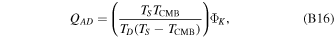
which is an energy-based definition that is basically equivalent to the usual formula, QAD ∼ 4π RC 2 kC (d Ta /d r), derived from Fourier's law.
Appendix C: Magnetic Diffusion Time
We determine the time it takes for the field to decay after convection ceases following the procedure detailed in Stevenson (2003) to approximate the magnetic diffusion time:
Here RC is the radius of the electrically conducting region (i.e., the core), and λ is the magnetic diffusivity given by

where μ0 is the permeability of free space, and σ is the electrical conductivity. We assume λ ∼ 1 m2 s–1, appropriate for terrestrial planets with a liquid iron alloy core (e.g., Schubert & Soderlund 2011), such that the magnetic field will diffuse across the core in τ ∼ 400 yr.
Appendix D: Tables
Tables D1 and D2 define the constants and variables used in our models.
Table D1. Description of Model Constants
| Term | Description | Value |
|---|---|---|
| μ0 | Permeability of free space | 1.257 × 10⁻⁶ H·m−1 |
| G | Gravitational constant | 6.67 × 10⁻¹¹ m3 · kg−1·s−2 |
| R | Universal gas constant | 8.3145 J · K−1 · mol−1 |
| RM | Radius of the Moon | 1737 km |
| RC | Radius of the core | 350 km |
| Ω | Angular velocity of the Moon | 2.66 × 10⁻⁶ rad · s−1 |
| K0 | Effective modulus | 121.4 × 10⁹ Pa |
| K1 | Effective derivative of effective modulus | 5.787 1 |
| Aρ | Constant in density profile | 1.59 |
| ρ0 | Central density | 6477 kg · m−3 |
| P0 | Central pressure | 5.15 × 10⁹ Pa |
| MC | Mass of the core | 1.16 × 10²¹ kg |
| VC | Volume of the core | 3.95 × 10¹⁶ m3 |
| g | Gravitational acceleration near the CMB | 0.6311 m · s−2 |
| γ | Grüneisen parameter for the core | 1.65 |
| Cc | Specific heat of the core | 835 J · kg−1 · K−1 |
| ΔSC | Entropy of melting for the inner core | 200 J · K−1· kg−1 |
| αI | Coefficient of compositional expansion for enriching the outer core in sulfur | 2.3 |
| λK | Average decay constant for potassium-40 | 1.76 × 10⁻¹⁷ s−1 |
| HK | Heat production rate for potassium-40 | 4.2 × 10⁻¹⁴ W · kg−1 · ppm−1 |
| c | Constant of proportionality in Equations (5)–(7) | 0.63 |
| dTL /dc | Compositional dependence of liquidus temperature | −2500 K |
| dTL /dP | Pressure dependence of liquidus temperature | 3 × 10⁻⁸ K · Pa−1 |
Download table as: ASCIITypeset image
Table D2. Definition of Model Inputs and Outputs
| Variable | Definition | Values |
|---|---|---|
| Input Parameters | ||
| [S] | Abundance of sulfur in the core a | 1–6 wt% |
| [K] | Abundance of potassium in the core b | 0–50 ppm |
| kC | Thermal conductivity of the core c | 10–50 W m−1 K−1 |
| QC | Present-day heat flow across the CMB d | 0–2 GW |
| Energy budget outputs of the core | ||
| QCMB | Heat flow across the CMB | GW |
| QL | Latent heat from inner core nucleation | GW |
| QG | Gravitational energy released from inner core nucleation | GW |
| QR | Radiogenic heating in the core | GW |
| QS | Secular cooling of the core | GW |
| Entropy Budget Outputs of the Core | ||
| ΦCMB | Dissipation available to power a dynamo | MW |
| ΦL | Dissipation associated with latent heat | MW |
| ΦG | Dissipation associated with gravitational energy | MW |
| ΦR | Dissipation associated with radiogenic heating | MW |
| ΦS | Dissipation associated with secular cooling | MW |
| ΦK | Dissipation sink associated with thermal conductivity | MW |
Notes.
a Weber et al. (2011). b Laneuville et al. (2014); Scheinberg et al. (2015); Hirose et al. (2013). c Pommier (2018). d Laneuville et al. (2014).Download table as: ASCIITypeset image