Constraining the Venus Interior Structure with Future VERITAS Measurements of the Gravitational Atmospheric Loading

The next decade will be the decade of Venus. The missions recently selected by NASA and ESA (VERITAS, DAVINCI, and EnVision) aim to radically advance our understanding of Earth's neighboring planet. The questions of the scientific community pushing for renewing and updating the available data sets of Venus are compelling. For instance, Venus' interior structure has not been probed by a planetary mission since the conclusion of the Magellan mission in 1994. The data sets gathered by Magellan were revolutionary for the time, but now fall far behind in terms of accuracy, resolution, and detail when compared to our knowledge of the other terrestrial bodies of the solar system and the capability of current planetary missions instrumentation. Venus and its remaining mysteries represent a central comparative case toward understanding the key elements determining (exo)planetary habitability (Way et al. 2016; Kane et al. 2019).

VERITAS (Venus Emissivity, Radio science, InSAR, Topography, And Spectroscopy; Smrekar et al. 2022) will conduct a gravity science investigation mainly devoted to the measurement of the gravity field, the solid-body tidal response, and the rotational state of Venus. It is ultimately aimed at refining our understanding of the interior structure of the planet. The radio tracking system of VERITAS, enabling the gravity science experiment, is designed to deliver a sensitivity that is improved by orders of magnitude with respect to what NASA's Magellan was able to achieve. This improved sensitivity gives access to dynamical effects that were already present in the Magellan data, but were below the noise floor. As recently pointed out by Goossens et al. (2018) and Bills et al. (2020), a reduced noise floor in the tracking data would reveal the gravitational signature of the complex interplay between the thick Venusian atmosphere and the solid planetary body through the mechanism of the atmospheric thermal tides. This global atmospheric mechanism manifests itself (gravitationally speaking) both directly in the net gravity anomaly that is produced by the displacement of atmospheric mass, and indirectly with the response of the solid planet to this moving gravitational normal load on its surface. Petricca et al. (2022) showed that the gravitational response to the atmospheric loading strongly depends on the interior properties of the planet through the loading Love numbers, and suggested that its measurement will provide significant constraints on the inversion of Venus' interior structure.

It has previously been shown that VERITAS gravity measurements will be sensitive to this phenomenon (Cascioli et al. 2021). This previous study, however, concentrated on demonstrating that an imperfect knowledge of the atmospheric thermal tides would not compromise the scientific objectives of VERITAS. Here, we change our perspective and investigate whether VERITAS could take advantage of its sensitivity to the atmospheric dynamics. We assess the capability and quality of a measurement of Venus' response to the atmospheric loading (i.e., the loading Love numbers ${k}_{l}^{{\prime} }$) and evaluate the importance of these measurements for producing additional constraints on the interior structure of Venus.

Precise knowledge of Venus' interior structure is essential to solving major outstanding questions about the evolution of rocky planets. Key questions include the following: What is the composition of initial accretionary material? Why does Venus lack a dynamo-driven magnetic field? How did early differentiation processes affect the core size and state and the mantle structure? Absent Earth-like plate tectonics, what is Venus' geodynamic system? Specifically, how do interior structure and heat loss couple to observable surface geology and atmospheric composition and evolution?

The composition, phase, and convective state of the core govern how much heat is lost from the core into the mantle. A better knowledge of the core and the core-mantle boundary is needed to discriminate between hypotheses to explain why Venus has no measurable dynamo today (Jacobson et al. 2017). Nimmo (2002) proposed that Venus lacks core convection and a dynamo because heat is not lost rapidly enough through the mantle and lithosphere due to the absence of plate tectonics. O'Rourke et al. (2018) hypothesized that Venus could have a basal magma ocean that suppresses heat flow from the core. The nature of the core-mantle boundary and core heat loss is also critical for understanding the origin of the ∼10 large mantle plumes that appear to be active today (e.g., Smrekar & Sotin 2012). An additional major question is why Venus exhibits two scales of mantle plumes. The large volcanic rises are similar in scale and surface features to Earth's mantle plume features, e.g., on Hawaii. Hundreds of smaller-scale features called coronae, with an average diameter of a few hundred kilometers, also occur, however. Could they also originate at the core-mantle boundary (Jellinek 2002), or do they require an additional, shallower transition zone or interface? Why are they unique to Venus?

On Earth, plate tectonics shapes Earth's long-term climate and volatile budget via volcanic outgassing and recycling of material into the mantle via subduction. An essential question for Venus is whether surface volcanism is largely constant over time or if there was a past "catastrophic" event. Catastrophic resurfacing motivates the hypothesis of episodic plate tectonics (or mobile lid convection), which would allow for past periods of mobile lid activity and high heat flow, leading to a current period of stagnant lid convection and lower heat flow. Mantle viscosity and lithospheric strength, a function of mantle heat flow, are the driving parameters for mobile lid versus stagnant lid behavior, as well as for volcanism. Many have advocated for an episodic mobile lid (e.g., Rolf et al. 2018; Weller & Kiefer 2020), but other styles of a stagnant lid convection are possible, such as a sluggish lid (Davaille et al. 2017) or squishy lid regimes (Lourenço et al. 2020), incorporating evidence for likely active subduction and volcanism. Constraints on mantle viscosity and structure are needed to refine these hypotheses and discriminate between geodynamic models.

The aim of this work is to demonstrate that VERITAS will be able to measure the Venus loading Love numbers and to assess the importance of their retrieved values for gaining more information on the planet's interior structure. To this end, we review the latest published models of the Venus deep interior and use them to compute the range of expected values of the tidal and loading Love numbers of Venus under different assumptions regarding core state, radius, mantle viscosity, and temperature profile. We simulate the mission scenario by embedding several sources of possible model errors to determine VERITAS' sensitivity to the load Love numbers in a robust manner. Finally, we assess the relevance of these estimates for providing improved constraints on Venus' interior.

This manuscript is structured as follows: in Section 2 we discuss the gravitational signature of the atmospheric thermal tides and their modeling. In Section 3 we detail the method we used to compute the tidal and loading Love numbers of Venus and discuss their relation to the interior structure. Section 4 follows with a discussion of how the loading Love numbers can be measured by VERITAS and the description and results of the numerical simulations we used to assess the sensitivity to these parameters. Section 5 comments on the implication of VERITAS measurements in terms of constraints on Venus' interior structure, and finally, Section 6 provides concluding remarks.

Venus rotates in a retrograde direction with a period of ∼243 days and has an orbital period of ∼224 days. The difference between these two periods gives rise to a solar day with a duration T_S = 116.752 days. The radiative input of the Sun on the atmosphere determines a hotter zone in proximity of the subsolar point and a cooler zone in the opposite hemisphere. This temperature dichotomy of the atmosphere gives rise to a mass transport phenomenon known as atmospheric thermal tide. The atmosphere near the subsolar point is hotter than the average and thus expands (i.e., the density is lower), while on the opposite hemisphere, the opposite occurs (Gold & Soter 1971; Dobrovolskis & Ingersoll 1980). Thus, in principle, the solar input creates a stable atmospheric thermal tide that rotates with respect to the body-fixed frame with a period equal to the solar day. The phenomenon, however, is more complex than this simple description, as the pressure field strongly depends on the topography of the Venus surface (see Figure 1). Moreover, the total gravitational perturbation is affected by other small-scale atmospheric waves. However, the contribution of the planetary-scale thermal tides to the gravity field is by far the largest (Bills et al. 2020; Petricca et al. 2022). The total gravitational signal is due to both the direct contribution (net transport of mass) and the modification of the solid-body gravitational potential due to atmospheric loading on the surface (Wahr et al. 1998). To correctly compute the gravitational signal due to the atmospheric dynamics, then, a precise global circulation model (GCM) is needed. In this work, we use the same atmospheric gravity field model as Goossens et al. (2017, 2018), which is derived from pressure field simulations by Garate-Lopez et al. (2018). Since we are interested in the estimation of the low-degree (i.e., large spatial scale) loading Love numbers, we assume that the total gravitational perturbation is only due to thermal tides. Admittedly, the current Venus GCMs are not necessarily tailored to deliver a fine description of the surface pressure anomalies, the main quantity driving our modeling of the gravitational signal of the tides, mainly because of the scarcity of in situ measurements and of the strong effect that poorly constrained parameters such as the shortwave heating rate of the lower haze below the cloud deck, the ground thermal inertia, or the cloud-top altitude at high latitudes can have on the low-atmosphere dynamics (e.g., Garate-Lopez & Lebonnois 2018; Navarro et al. 2023). Indeed, in our work we rely on the GCM predictions, but try to mitigate the model dependence of the results by exploring different perturbed realizations of the surface pressure fields (see Section 4.1), allowing for a more robust interpretation.

Zoom In Zoom Out Reset image size

The GCM model has been evaluated with a sampling of 1 Venus hour (i.e., 24 total samples over 116.752 Earth days) in a 1° × 1° grid. We define the pressure anomaly ΔP as

$$\begin{eqnarray}&&{\rm{\Delta }}P\left(t,\vartheta ,\varphi \right)=P\left(t,\vartheta ,\varphi \right)-\left\langle P\left(t,\vartheta ,\varphi \right)\right\rangle ,\end{eqnarray} \tag{ 1 }$$

where P denotes the pressure field, t, ϑ, and φ are the time, latitude, and longitude, respectively, and $\left\langle \cdot \right\rangle$ is the time-average operator. Figure 1 shows the pressure anomaly field at local solar times (LST) of 12 hr, 18 hr, 24 hr, and 6h at the prime meridian (0° longitude). The pressure anomaly field shows peaks on the order of 1kPa, corresponding to ∼103ppm of the average surface pressure of Venus (96 atm). For a convenient comparison with the static gravitational potential, it is useful to represent the pressure anomaly field in a spherical harmonics series expansion. We use the standard spherical harmonics 4π normalization (e.g., Kaula 1966), defined by the inner product (over the unitary sphere Ω) between two spherical harmonics base functions Y_lm of degree l and order m such that

$$\begin{eqnarray}&&\int \,{Y}_{{lm}}{Y}_{{l}^{{\prime} }{m}^{{\prime} }}d{\rm{\Omega }}=4\pi {\delta }_{{{ll}}^{{\prime} }}{\delta }_{{{mm}}^{{\prime} }}\end{eqnarray} \tag{ 2 }$$

where δ_ij denotes the Kronecker delta operator.

Using this procedure, we can obtain the Stokes coefficients of the spherical harmonics representation of the pressure anomaly ${\rm{\Delta }}{C}_{{lm}}^{\mathrm{atm}}$ and ${\rm{\Delta }}{S}_{{lm}}^{\mathrm{atm}}$ for each time sample, and thus build a time series of the variation of each individual coefficient.

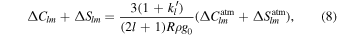
The transformation from atmospheric pressure anomaly to its gravitational potential counterpart is obtained through Wahr et al. (1998; we refer to Petricca et al. (2022) for a thorough discussion of the topic),

$$\begin{eqnarray}&&{\rm{\Delta }}{C}_{{lm}}\left(t\right)=\displaystyle \frac{3\left(1+{k}_{l}^{{\prime} }\right)}{\left(2l+1\right)R\rho {g}_{0}}{\rm{\Delta }}{C}_{{lm}}^{\mathrm{atm}}\left(t\right)\end{eqnarray} \tag{ 3a }$$

$$\begin{eqnarray}&&{\rm{\Delta }}{S}_{{lm}}\left(t\right)=\displaystyle \frac{3\left(1+{k}_{l}^{{\prime} }\right)}{\left(2l+1\right)R\rho {g}_{0}}{\rm{\Delta }}{S}_{{lm}}^{\mathrm{atm}}\left(t\right),\end{eqnarray} \tag{ 3b }$$

where R, ρ, and g₀ are the planetary radius, mean density, and surface gravity acceleration, respectively. ${k}_{l}^{{\prime} }$ are called the loading Love numbers of degree l. Similarly to tidal Love numbers (k_l ), these are nondimensional coefficients relating the forcing potential and the planet's response (Love 1911). While the tidal Love numbers relate a perturbing gravitational potential (forcing) to the modification of the gravitational potential of the perturbed body (response), the loading Love numbers relate the application of a gravitational normal load to the induced modification of the perturbed body gravitational potential. It is clear then from Equations (3a) and (3b) that the atmosphere-induced gravitational perturbation can be seen as acting in two different ways. We can identify a direct effect that is due to the redistribution of atmospheric masses (the 1 in the $\left(1+{k}_{l}^{{\prime} }\right)$ term in Equations (3a) and (3b), and an indirect effect that is due to the response of the planetary body to the normal loading (${k}_{l}^{{\prime} }$ in the $\left(1+{k}_{l}^{{\prime} }\right)$ term in Equations (3a) and (3b)). To assess the magnitude of the gravity anomaly induced by the atmospheric mass redistribution, it is convenient to compute the amplitude spectrum of the time-variable atmospheric anomaly gravity field (C_l in Equation (2.39) of Bertotti et al. 2003). Being a periodic phenomenon, as pointed out by Bills et al. (2020), the spectrum of the atmospheric anomaly gravity field is time-invariant; indeed, it will convey the same information regardless of the time stamp chosen for its computation. Figure 2 reports the comparison between the amplitude spectrum of Venus' static gravity field, as measured by Magellan (MGN180U; Konopliv et al. 1999) and its associated uncertainty, the uncertainty attainable by VERITAS (as simulated by Mazarico et al. 2019), and the computed spectrum of gravity anomalies induced by atmospheric mass redistribution.

Zoom In Zoom Out Reset image size

Figure 2 clearly shows that the gravitational signal of the atmosphere was beyond Magellan's reach, but will be above the noise floor attainable by VERITAS. This fact justifies the efforts made to study this phenomenon and assess whether the atmospheric signal, if not properly modeled, might bias the gravity science experiment results. It must be noted, however, that the comparison between spectra is not an exact measure of what will be effectively measurable. While it is generally true that a phenomenon whose amplitude spectrum is orders of magnitude above the uncertainty will surely be detectable, this approach cannot be used for definitive quantitative estimates in more subtle cases like that of VERITAS, thus justifying and motivating the need of detailed numerical simulations. In previous work (Cascioli et al. 2021), it has been shown that VERITAS will be sensitive to the atmospheric signal and that with proper data-analysis strategies, the errors due to an imperfect knowledge of the atmospheric dynamics can be absorbed in the data reduction process without impacting the objectives of the gravity science experiment. More interestingly, because the expected gravitational signal is higher than the measurement noise floor of VERITAS, it could be possible to probe the main dynamical processes generating it. Equations (3a) and (3b) show the strong dependence of the gravitational signal to the loading Love numbers, which in turn depend on the interior structure of the planet (see Section 3). Measured loading Love numbers, in combination with the measurement of the tidal Love number k₂ (real and imaginary parts) and the moment of inertia factor (MOIF), could then impose new and tighter constraints on the interior knowledge.

To determine theoretical values for the Venus' loading Love numbers and tidal Love numbers, we must first find a solution to the viscoelastic-gravitational problem within the planet (Takeuchi & Saito 1972). This method has been employed in the study of icy moons (Tobie et al. 2005; Beuthe 2015), Mercury (Mazarico et al. 2014; Goossens et al. 2022), Earth (Martens 2016), and exoplanets (Bolmont et al. 2020). It assumes spherical symmetry (parameters such as density may only vary with radius) and can describe self-gravitating deformations from a variety of sources (tides, surface loading, quakes, or centrifugal flattening). Both the equations of motion and Poisson's equations can be cast into a set of four (for liquid layers; see Equations (11)–(14) of Kamata et al. 2015) or six (for solid layers; see Equations (4)–(9) of Kamata et al. 2015) ordinary differential equations that are solved as a system starting from the center of the planet. It is common practice to introduce radial functions, y_i (i ∈ [1, 6]), to perform these calculations. y₁ and y₃ are associated with the radial and tangential displacements, respectively, while y₂ and y₄ are used to find the radial stresses. The total gravitational potential inside the planet is provided by scaling the surface-applied potential by y₅. Finally, y₆ is defined to assist in the application of the surface boundary conditions while maintaining a continuous gravitational potential. The Love numbers are found using the following relations on these functions, calculated for either the tidal or loading surface conditions (e.g., Beuthe 2015),

$$\begin{eqnarray}&&h={{gy}}_{1}\left(R\right)\end{eqnarray} \tag{ 4a }$$

$$\begin{eqnarray}&&l={{gy}}_{3}\left(R\right)\end{eqnarray} \tag{ 4b }$$

$$\begin{eqnarray}&&k={y}_{5}\left(R\right)-1,\end{eqnarray} \tag{ 4c }$$

where g is the acceleration due to gravity at the surface, and h, l, and k are the radial, tangential, and gravitational Love numbers, respectively (Love 1911). For a viscoelastic planet, the radial y_i functions are complex-valued; their imaginary parts exist due to the dissipation of energy via frictional heating during tidal or surface loading (see Bagheri et al. 2022, and references therein). These imaginary parts are passed along to the Love numbers and can be used as additional observational constraints if the phase (i.e., the angular representation of its complex part) of a given Love number can be measured with reasonable precision (e.g., Dumoulin et al. 2017; Cascioli et al.2021).

3.1. Solving the Viscoelastic-gravitational Problem

Several methods have been developed to find the solutions for y_i within a planet, such as the propagator matrix method (e.g., Jara-Orué & Vermeersen 2011; Sabadini & Vermeersen 2004) and the shooting method (e.g., Bolmont et al. 2020; Tobie et al. 2005). We choose to use the latter approach as it readily allows for the effects due to compressibility (determined by a finite bulk modulus) to be explored in a computationally stable way (e.g., Beuthe 2015; Martens 2016; Bolmont et al. 2020). We have found compressibility to be an important consideration for a planet like Venus, especially for the calculation of the loading Love numbers. For example, Figure 3 shows the tidal versus loading Love number ${k}_{2}^{{\prime} }$ calculated for the suite of interior models explored in this work (described in Section 3.2) under the compressible and incompressible assumptions. Previous studies such as Petricca et al. (2022) did not consider the effect of compressibility. By considering compressibility, we observed tidal Love numbers that are larger by ∼4% on average and loading Love numbers that are lower by ∼23%. These differences are larger than the expected measurement uncertainty we calculate in Section 4.2 (see also Table 3).

Zoom In Zoom Out Reset image size

Performing the Love number calculations using the shooting method requires first finding a set of solutions to the viscoelastic-gravitational differential equations starting with initial values at the planet center. These initial values are provided, for example, by Equations (100)–(103) in Takeuchi & Saito (1972) and depend on the local density as well as the shear and bulk moduli of the central core. For solid layers, only three of the solutions are regular at r = 0, requiring three different starting solutions. For static ⁶ liquid layers, there is only one regular solution, and its starting values are provided by Equation (19) of Saito (1974). Numerical integration of these equations is performed until a phase interface is reached. Interfaces between liquid and solid layers require the multiple solutions to be connected through unknown constants of integration, as well as knowledge about the physical properties of the layers, as described in Section 3 of Takeuchi & Saito (1972). These unknown constants are then propagated through the superposition of solutions up to the surface where they are determined by boundary conditions. These boundary conditions vary depending on whether we are calculating the tidal or loading Love numbers (see Table 1).

Table 1. Surface Boundary Conditions Used to Calculate the Tidal and Loading Love Numbers (Beuthe 2015)

	Tidal Love Numbers	Loading Love Numbers
y2(R)	0	$-\tfrac{2l+1}{3}{\rho }_{\mathrm{bulk}}$
y4(R)	0	0
y6(R)	$\tfrac{2l+1}{R}$	$\tfrac{2l+1}{R}$

Note. In addition to the planet's mean radius, R, and the planet's bulk density, ρ_bulk, the Love numbers also depend on the harmonic degree, l, which in the context of tidal dissipation and surface loading is a positive valued integer greater than 0.

Download table as:  ASCIITypeset image

We performed these numerical integrations using the TidalPy software package (Renaud 2022), which uses a fifth-order Runge–Kutta ordinary differential equation integrator with adaptive step sizing.

3.2. Interior Structure of Venus

Before these calculations can be made, we must first define the interior structure and physical properties of Venus, including the density and shear and the bulk moduli as a function of radius. In the case of a viscoelastic planet, the moduli may take the form of complex numbers. In this work, we focus on the effects of shear dissipation and assume that the bulk modulus is purely real valued. ⁷ To calculate the complex shear modulus, we use the Andrade rheology (Andrade 1910; Castillo-Rogez et al. 2011; Renaud & Henning 2018), which relates the complex shear modulus $\tilde{\mu }$ to the static shear μ, viscosity η, forcing frequency ω, and material properties,

$$\begin{eqnarray}&&\displaystyle \frac{1}{\tilde{\mu }}=\displaystyle \frac{1}{\mu }-\displaystyle \frac{i}{\eta \omega }+\displaystyle \frac{{\left(i\eta \zeta \omega /\mu \right)}^{-\alpha }}{\mu }{\rm{\Gamma }}\left(\alpha +1\right),\end{eqnarray} \tag{ 5 }$$

where i is the imaginary number, and Γ is the Gamma function. The forcing frequency in the case of surface loading is largely driven by atmospheric changes occurring at a period of 116.752 Earth days. Additional material properties of a planet's bulk are parameterized in the Andrade rheology via two dimensionless variables α and ζ (Efroimsky 2012). α in part describes the slope of the shear response versus forcing frequency and viscosity, while ζ is the ratio of the characteristic timescales of anelastic and viscoelastic creep (Renaud & Henning 2018). Much more experimental work is required to better understand these parameters and any additional dependences they may share. However, for the silicate materials of which we expect the bulk of Venus' interior to be comprised, studies have found that α and ζ to range between 0.2–0.6 and 0.1–10, respectively. We use the values of α = 0.3 and ζ = 1 for our calculations, which represent reasonable midpoints in the experimental literature (see Renaud 2019, and the references therein for a review). In Section 5.1 we briefly discuss the impact that the Sundberg–Cooper rheology (Sundberg & Cooper 2010) may have on Venus' response. We refer to Renaud & Henning (2018) for a detailed description of this model, but note that the key difference between it and the Andrade model described by Equation (5) is an additional Debye-like dissipation peak in both frequency and viscosity space.

Either rheology requires Venus' mantle and core viscosity and shear modulus as inputs, but these properties are currently unknown. Prior work has attempted to model them by performing extrapolations from the preliminary Earth reference model (PREM; Dziewonski & Anderson 1981; Aitta 2012) as well as using equations of state on the anticipated interior composition and thermal state of Venus. In this work, we use the interior profiles produced by Xiao et al. (2021; hereafter X21), who considered many different interior configurations, including the presence or lack of a solid inner core, and the data produced by Dumoulin et al. (2017; from now on D17; the data were provided by the authors; see the Acknowledgment) assuming a purely liquid core. X21 explored 12 main variations on Venus' interior based on whether a solid inner core was present, a cold versus hot mantle (the main difference being the presence of a thick basalt layer in the mantle for the cold case; see O'Rourke et al. 2018), and three different parameters used to calculate the mantle viscosity. Each model then had 100 (solid inner core) or 300 (purely liquid core) simulations, where each simulation explored variations in the core-mantle boundary (CMB) temperature (3200–4600 K), the thermal boundary layer thickness (10–200 km), the mantle transition layer thickness (solid inner core only; 10–200 km), the core sulfur (0–11.8 wt%) and silicon content (0 to 1-χ_Fe12S), and the CMB radius (3047–3310 km). D17 also explored a hot and cold mantle for Venus as well as differences in internal composition (see Tables 1 and 2 in D17) and CMB radius (2941–3425 km). We use six cases explored by D17, all of which consider a purely liquid core. Unlike X21, D17 does not prescribe a mantle viscosity for their simulations. For these models, we instead use a viscosity that is constant throughout the mantle, and we rerun the Love number calculations with a different constant viscosity chosen from the range 10¹⁸–10²² Pa s. As with D17 and X21, we do not consider the case that Venus' core is entirely solid in this work.

Table 2. The Average Value and Overall Spread of the Tidal k_l and Loading ${k}_{l}^{{\prime} }$ Love Numbers Are Based on Calculations Performed on the X21 Simulation Results for Purely Liquid Core and Solid Inner Core Models

		Tidal				Loading
		Re$\left[{k}_{l}\right]$		-Im$\left[{k}_{l}\right]$		Re$\left[{k}_{l}^{{\prime} }\right]$
Purely Liquid Core	l = 2	${0.3045}_{-0.0324}^{+0.0719}$	34.3%	${0.0182}_{-0.0157}^{+0.0504}$	362%	$-{0.3129}_{-0.0973}^{+0.0373}$	43.1%
	l = 3	${0.0950}_{-0.0115}^{+0.0268}$	40.3%	${0.0076}_{-0.0066}^{+0.0023}$	395%	$-{0.2051}_{-0.0816}^{+0.0297}$	54.3%
	l = 4	${0.0434}_{-0.0049}^{+0.0117}$	38.1%	${0.0037}_{-0.0031}^{+0.0108}$	378%	$-{0.1420}_{-0.0556}^{+0.0199}$	53.2%
	l = 5	${0.0258}_{-0.0025}^{+0.0057}$	31.9%	${0.0020}_{-0.0016}^{+0.0051}$	333%	$-{0.1120}_{-0.0368}^{+0.0139}$	45.2%
Solid Inner Core	l = 2	${0.2805}_{-0.0246}^{+0.0385}$	22.5%	${0.0095}_{-0.0072}^{+0.0172}$	256%	$-{0.2857}_{-0.0390}^{+0.0240}$	22.1%
	l = 3	${0.0869}_{-0.0081}^{+0.0133}$	24.6%	${0.0036}_{-0.0027}^{+0.0066}$	259%	$-{0.1839}_{-0.0302}^{+0.0179}$	26.2%
	l = 4	${0.0404}_{-0.0033}^{+0.0055}$	21.8%	${0.0019}_{-0.0014}^{+0.0031}$	234%	$-{0.1294}_{-0.0205}^{+0.0116}$	24.8%
	l = 5	${0.0246}_{-0.0017}^{+0.0028}$	18.5%	${0.0012}_{-0.0008}^{+0.0017}$	202%	$-{0.1049}_{-0.0144}^{+0.0086}$	21.9%

Note. The ranges are estimated by using the 5th and 95th percentile of simulation results, such that 90% of the findings lie within the provided ranges. The percentages were calculated as the difference between these percentiles divided by the average value to give a sense of the relative spread in values.

Download table as:  ASCIITypeset image

3.3. Loading Love Numbers of Venus

Using the methods described in Section 3.1, we calculate Venus' tidal (see Figures 4(a)–(d)) and loading Love numbers (see Figures 4(e)–(f)) for harmonic degrees l = 2 to l = 10. In this section, we differentiate by models that do and do not contain a solid inner core, as the analysis of the observed Love numbers, along with moment of inertia measurements, may help to constrain whether an inner core is present in modern Venus (in analogy to what has been done for Mars; e.g., Rivoldini et al. 2011). To perform a comparison between these core models, we choose to only show the simulations conducted by X21 and do not analyze the data from D17, who did not consider a solid inner core. This choice was also made as the X21 simulations use a self-consistent viscosity profile for the mantle (see Xiao et al. 2021 Equation (3)), rather than the constant and prescribed values used for D17. This allows us to look at the statistics of multiple simulation runs that range over various model inputs, as described in Section 3.2. The average and spread of the 600 X21 simulations (for a purely liquid and a solid inner core with varying size) are shown in Table 2.

Zoom In Zoom Out Reset image size

We find that the Love numbers, particularly at low harmonic degree, show moderate variations. We define the relative spread as the separation from the 5th to the 95th percentile of all the model values divided by the average value. The relative spread of k₂ for the liquid core models is higher than 34% (with a range of 0.272–0.376). This spread decreases slightly when a solid inner core is considered with a relative spread of 22.5% and a range of 0.256–0.319. The loading Love number ${k}_{2}^{{\prime} }$ is found to range between −0.410 to −0.276 (average value of −0.313 and relative spread of 43.1%) for a purely liquid core and between −0.325 to −0.262 (average value of −0.286 and relative variation of 22.1%) for a solid inner core. Petricca et al. (2022) found that for a liquid core, the loading Love numbers ranged between −0.340 to −0.210. Our lower ranges are consistent with the compressibility correction discussed in Section 3.1. Other differences, such as the larger spread in values, arise from our use of the X21 data compared to the use of D17 simulations in Petricca et al. (2022).

We confirm the findings of Petricca et al. (2022) that a lower mantle viscosity leads to lower loading Love numbers. The large spread in the values of the imaginary portion of the tidal Love number (200%–390% relative spread; see Table 2) suggests that a precise measurement of its value may go a long way to constrain the mantle viscosity, with less degeneracy than the real portion alone would provide. We also find that the loading Love number has a semiasymptotic relation with harmonic degree. It converges near −0.08 at high l with only a slight positive slope (see Figures 4(e) and (f)). These high degrees are thus not sensitive to and diagnostic of the interior structure.

To quantify the sensitivity of the VERITAS radiometric measurements to the loading Love numbers, we have run an extensive set of numerical simulations of the VERITAS gravity experiment aiming to assess the sensitivity of the tracking system and the robustness of the solution to possible uncertainties in the mismodeling of the atmospheric pressure field. The gravity science experiment is based on the collection of two-way coherent X- and Ka-band radiometric measurements. The radio tracking system of VERITAS has heritage from ESA's BepiColombo and will obtain an end-to-end accuracy ranging between 0.015 and 0.038 mm s⁻¹ at 10 s integration time (Cappuccio et al. 2020; Iess et al. 2021). In this work, we have implemented a noise model that accounts for all the main noise sources (solar plasma, Earth troposphere, ground station frequency stability, antenna mechanical noise, etc.) reflecting the latest results of BepiColombo. The model has been tuned to reflect the VERITAS requirement of an end-to-end noise of 0.033 mm s⁻¹ over 10 s integration times outside of solar conjunctions (Sun–Venus–Earth angle >15°). VERITAS will also collect radar tie points (repeated observations of the same surface feature) from the interferometric synthetic aperture radar VISAR (Hensley et al. 2020). The radar tie points will greatly contribute to the scientific return of the mission by strongly tying the motion of the probe to the rotational state of the planet, thus significantly increasing the sensitivity of the experiment to the planet's moment of inertia (Cascioli et al. 2021). The expected noise level for radar tie points is 10 HZ and 3 m for their Doppler and range components, respectively (see Cascioli et al. 2021, Appendix 1 for additional details). The numerical simulation setup, based on NASA-JPL MONTE (Evans et al. 2018), is identical to the one used in our previous works. We summarize the main features here. The orbit-determination (OD) problem is formulated in its multi-arc form (Milani & Gronchi 2009), meaning that the solved-for parameters are divided into two groups: local and global. The local parameters are those that influence a single data arc, while the global parameters have influence over the whole mission (e.g., the Venus gravity field). We subdivide the nominal mission time span (about four Venus sidereal days corresponding to ∼2.7 yr) into 324 arcs lasting three days each. We estimate the gravity field of Venus up to degree and order 50 (as higher degrees do not affect the estimate of long characteristic-time phenomena such as those we are interested in here), the tidal Love number k₂ (both real and imaginary), and the planetary body-fixed spin axis orientation and orientation-rate (precession) in addition to the atmospheric gravity field-related parameters discussed in the next section. We also estimate the sidereal period as a local parameter to account for possible short-term variability (Margot et al. 2021) and a scale factor per arc for the solar radiation pressure, and we model (and estimate) the drag coefficient as a stochastic parameter with an update time of 30 minutes. For a more details on the simulation and filter setup, we refer to Cascioli et al. (2021).

4.1. Measuring the Loading Love Numbers

The core of the gravity science experiment of VERITAS relies on the solution of an OD problem. An OD problem consists in finding the set of parameters of the dynamical model of the spacecraft (the state of the problem) that minimizes the discrepancy between the actual measurements collected by the ground station and radar (observed observables) and the measurements predicted through the chosen dynamical model (computed observables). In its linear least-squares formulation (for a detailed description, see Tapley et al. 2004 or Cascioli & Genova 2021), the minimum variance estimator of the state correction $\hat{x}$ is given by

$$\begin{eqnarray}&&\hat{x}=\left({H}^{T}{R}^{-1}H+{\overline{P}}^{-1}\right)\left({H}^{T}{R}^{-1}y+{\overline{P}}^{-1}\overline{x}\right),\end{eqnarray} \tag{ 6 }$$

where R is the covariance matrix of the measurement noise, $\overline{P}$ is the a priori covariance matrix of the state, $\overline{x}$ is the vector of a priori values of the state, and y is the vector of observation residuals (the difference between observed and computed observables). H is the so-called mapping matrix, which collects the partial derivatives of the observations with respect to the state. To include the estimation of the loading Love numbers in the OD filter, a suitable mathematical representation of the gravitational anomalies due to the atmosphere must be developed.

Leveraging the periodic nature of the atmospheric thermal tides, the time series of the pressure anomaly Stokes coefficients ${\rm{\Delta }}{C}_{{lm}}^{\mathrm{atm}}\left(t\right)$ and ${\rm{\Delta }}{S}_{{lm}}^{\mathrm{atm}}\left(t\right)$ can be expanded in Fourier series,

$$\begin{eqnarray}&&{\rm{\Delta }}{C}_{{lm}}^{\mathrm{atm}}(t)=\displaystyle \sum _{f}{A}_{{lm}}^{C}\cos \left(2\pi {ft}\right)+{B}_{{lm}}^{C}\sin \left(2\pi {ft}\right)\end{eqnarray} \tag{ 7a }$$

$$\begin{eqnarray}&&{\rm{\Delta }}{S}_{{lm}}^{\mathrm{atm}}(t)=\displaystyle \sum _{f}{A}_{{lm}}^{S}\cos \left(2\pi {ft}\right)+{B}_{{lm}}^{S}\sin \left(2\pi {ft}\right).\end{eqnarray} \tag{ 7b }$$

The summation is performed over harmonics of the forcing period T_s , i.e., at frequencies $f=\tfrac{1}{{T}_{S}},\tfrac{2}{{T}_{S}},\ldots ,\tfrac{N}{{T}_{S}}$. The Fourier expansion is limited by the number of samples extracted from the time series of the pressure grids. The harmonic representation of the gravity anomalies is very convenient for forward modeling the phenomenon, leaving the modeler the ability to easily disentangle and select the different frequency contents of the signal.

Since the same ${k}_{l}^{{\prime} }$ holds for both ΔC_lm (t) and ΔS_lm (t), Equations (3a) and (3b) can be summed together,

$$\begin{eqnarray}&&{\rm{\Delta }}{C}_{{lm}}+{\rm{\Delta }}{S}_{{lm}}=\displaystyle \frac{3\left(1+{k}_{l}^{{\prime} }\right)}{\left(2l+1\right)R\rho {g}_{0}}\left({\rm{\Delta }}{C}_{{lm}}^{\mathrm{atm}}+{\rm{\Delta }}{S}_{{lm}}^{\mathrm{atm}}\right),\end{eqnarray} \tag{ 8 }$$

from which the partial derivative of the measurement y with respect to the loading Love number of degree l is computed applying the chain rule,

$$\begin{eqnarray}&&\displaystyle \frac{\partial y}{\partial {k}_{l}^{{\prime} }}=\displaystyle \sum _{m}\displaystyle \frac{\partial y}{\partial {\rm{\Delta }}{C}_{{lm}}}\displaystyle \frac{\partial {\rm{\Delta }}{C}_{{lm}}}{\partial {k}_{l}^{{\prime} }}+\displaystyle \frac{\partial y}{\partial {\rm{\Delta }}{S}_{{lm}}}\displaystyle \frac{\partial {\rm{\Delta }}{S}_{{lm}}}{\partial {k}_{l}^{{\prime} }},\end{eqnarray} \tag{ 9 }$$

where

$$\begin{eqnarray}&&\displaystyle \frac{\partial {\rm{\Delta }}{C}_{{lm}}}{\partial {k}_{l}^{{\prime} }}=\displaystyle \frac{3}{\left(2l+1\right)R\rho {g}_{0}}{\rm{\Delta }}{C}_{{lm}}^{\mathrm{atm}}\end{eqnarray} \tag{ 10a }$$

$$\begin{eqnarray}&&\displaystyle \frac{\partial {\rm{\Delta }}{S}_{{lm}}}{\partial {k}_{l}^{{\prime} }}=\displaystyle \frac{3}{\left(2l+1\right)R\rho {g}_{0}}{\rm{\Delta }}{S}_{{lm}}^{\mathrm{atm}}.\end{eqnarray} \tag{ 10b }$$

The terms $\tfrac{\partial y}{\partial {\rm{\Delta }}{C}_{{lm}}}$ and $\tfrac{\partial y}{\partial {\rm{\Delta }}{S}_{{lm}}}$ can be computed by observing that the instantaneous partial derivative of the observable with respect to ΔC_lm and ΔS_lm is identical to the partial derivative with respect to static C_lm and S_lm . The latter are very well known and already implemented in the majority of OD codes (e.g., Moyer 2003).

Equation (9) has to be evaluated at the epoch of each observation, which in general will differ from the time samples of the pressure grids obtained from the GCM. The values of ${\rm{\Delta }}{C}_{{lm}}^{\mathrm{atm}}$ and ${\rm{\Delta }}{S}_{{lm}}^{\mathrm{atm}}$ on the right-hand side of Equation (10a) and (10b) are thus computed from their Fourier series expansion.

With this procedure, we add the loading Love numbers up to degree 5 to the OD filter as global parameters. We choose degree 5 as a cutoff after having verified through preliminary simulations that higher degrees are not measurable due to the low signal-to-noise ratio (see also Figure 2). As evidenced by Equations (3a) and (3b), the gravity anomalies induced by the atmospheric mass redistribution do not depend on the loading Love numbers alone and are strongly driven by the underlying forcing atmospheric pressure field. The assumption that the uncertainty of the estimated ${k}_{l}^{{\prime} }$ matches their formal errors extracted from the OD filter might lead to an underestimation of the propagation of GCM uncertainties. Recent studies show a good match between the structure of the thermal tides predicted by GCMs and the in situ measurements collected by Venus Express VIRTIS (Scarica et al. 2019) for altitudes >60 km. However, the amplitude of the uncertainty or error expected in atmospheric pressure anomaly fields at the surface has not been similarly ascertained. For this reason, in our simulations, we perturb both the atmospheric pressure field and the static body gravity field. This implies that we use the nominal models to generate the synthetic observables used as truth in the orbit determination procedure and the perturbed models in the retrieval process. In the following, we will report both the formal uncertainty and the estimation error (difference between estimate and truth), which more realistically reflects the true attainable uncertainty.

In our simulation, the static gravity field measured by Magellan has been perturbed from its measured covariance (Konopliv et al. 1999). For what pertains to the atmospheric pressure field, we have run different cases to quantify the effect of possible GCM mismodeling. We identified two main ways of perturbing the atmospheric pressure anomaly field: perturbing the pressure grid prior to its expansion into spherical harmonics and Fourier series, and directly perturbing the Fourier series coefficients. Comparisons between GCM predictions and in situ observations have shown thermal anomaly differences on the order of 5–10 K at an altitude of ∼60 km (Scarica et al. 2019). These differences map into relative variations in the pressure anomalies on the order of 1%. Because of the very different mechanisms regulating the surface pressure and the cloud region (∼60 km), a direct extrapolation of these comparison studies cannot be adopted. Thus, we have chosen a conservative approach and adopt perturbations of 10% on the pressure anomaly grids for our simulations.

Because of their different nature, the two perturbation methods lead to different magnitudes of the resulting perturbed gravity anomalies. To obtain the same effect of perturbing the pressure grid at the 10% level, the Fourier coefficients need to be perturbed at the 2% level. Figure 5 shows the relative difference in the gravity anomalies using the two perturbation methods. It is interesting to highlight the difference between the two methods: directly perturbing the pressure grid (Figure 5, top panel) consists of applying a near-white noise over the whole grid, thus locally perturbing the atmospheric value while maintaining the underlying pressure anomaly geospatial structure. On the other hand, perturbing the Fourier expansion coefficients results in a modification of the spatio-temporal structure of the pressure anomaly field, which may better mimic mismodeling of the physical processes embedded in the GCM models.

Zoom In Zoom Out Reset image size

4.2. Results

We run the numerical simulations for the two distinct perturbation cases discussed in the previous paragraph. From now on, we refer to the pressure grid perturbation as Solution P (SOL-P) and to the Fourier coefficient perturbation as Solution F (SOL-F). We first simulate the gravity experiment using Doppler tracking only (no radar tie points) to prove the capability of measuring the loading Love numbers with Doppler data alone. A discussion of the attainable results when performing a combined Doppler and tie points analysis will follow shortly after.

We have run a full recovery study (not a covariance analysis) to probe the systematic errors introduced after perturbing the atmospheric input and other parameters such as the loading Love numbers and the static gravity field coefficients. In a covariance simulation, only the formal estimation uncertainty of the parameters is recovered; in a full simulation, all the parameters are initially perturbed, and thus the estimation errors are also obtained, which account for the effect of systematic effects and correlations. Table 3 reports the simulation results in terms of formal uncertainty and estimation error on the parameters of interest. The orbit determination solution is shown to be robust to this magnitude of atmospheric perturbation, as testified by the generally good quality of the fit. We find that the estimation errors are comparable with the formal uncertainties. As expected, the radiometric observables are mainly sensitive to the degree 2 loading Love number ${k}_{2}^{{\prime} }$, whose expected error, which we choose as the maximum between the formal uncertainty and estimation error for SOL-P and SOL-F, corresponds to a spread of 9.7% compared to the ${k}_{2}^{{\prime} }$ range (5th–95th percentile) predicted by the various interior models we tested (see Table 2). The degrees 3 and 4 are less strongly recovered, while ${k}_{5}^{{\prime} }$ is not resolved as its uncertainty is larger than the modeled range (>100%). These results suggest that the measurement of ${k}_{2}^{{\prime} }$ (and more marginally, ${k}_{3}^{{\prime} }$ and ${k}_{4}^{{\prime} }$) could help in discriminating between plausible interior structure models.

Table 3. Formal Uncertainties and Estimation Errors on the Main Parameters of Interest in the Two Simulated Doppler- only Cases (SOL-P and SOL-F) and Formal Uncertainties in the Doppler + Tie Points Case.

	Doppler only				Doppler + Tie Points
		Solution P	Solution F
Parameter	Formal Uncertainty	Estimation Error	Estimation Error	Percentage of max. Variability	Formal Uncertainty	Percentage of max. Variability
$\mathrm{Re}[{{\rm{k}}}_{2}]$	4.0 × 10−4	5.3 × 10−4	7.1 × 10−4	⋯	1.2 × 10−4	⋯
$\mathrm{Im}[{{\rm{k}}}_{2}]$	3.9 × 10−4	4.6 × 10−4	3.9 × 10−4	⋯	1.2 × 10−4	⋯
MOIF	4.3 × 10−3	9.0 × 10−4	8.5 × 10−4	⋯	5.0 × 10−4	⋯
${k}_{2}^{{\prime} }$	1.3 × 10−2	8.0 × 10−3	6.3 × 10−3	9.7%	5.0 × 10−3	3.7%
${k}_{3}^{{\prime} }$	5.0 × 10−2	4.2 × 10−2	4.8 × 10−2	45%	4.0 × 10−2	35%
${k}_{4}^{{\prime} }$	3.2 × 10−2	2.0 × 10−3	4.7 × 10−2	62%	1.3 × 10−2	17%
${k}_{5}^{{\prime} }$	6.8 × 10−2	8.8 × 10−2	9.6 × 10−3	170%	4.0 × 10−2	79%

Note. We also report the expected uncertainty (the maximum between the formal uncertainty and the estimation error P and F) as a percentage of the maximum expected variability of the loading Love numbers (defined as the width of the 5th–95th percentiles, as discussed in Section 3 ).

Download table as:  ASCIITypeset image

As discussed in previous work (Cascioli et al. 2021), the combined analysis of Doppler tracking and radar tie points can substantially augment the sensitivity to the rotational state of the planet, leading to a reduction in the uncertainty on the moment of inertia factor (MOIF) of nearly an order of magnitude. The inclusion of tie points in the analysis has the beneficial effect of strengthening the trajectory reconstruction of the probe through a better determination of the parameters related to nongravitational forces in the filter, particularly by bringing new measurements outside of the radio tracking periods (Cascioli et al. 2022). This process has been proven to benefit the retrieval of the Love numbers as well, with a reduction in the uncertainties of the tidal Love number and the associated tidal lag of a factor of 2–3. Having demonstrated that the OD filter can consistently recover perturbations in the atmospheric model, we report in Table 3 the results of a covariance simulation using the combination of Doppler and tie points (because of the dramatic increase in computational expense of a full perturbed inversion when using tie points, we only performed a covariance simulation, with resulting formal uncertainty values, but no derived biasing errors). The inclusion of tie points enables a reduction of the uncertainty of ${k}_{2}^{{\prime} }$ by a factor of ∼2.5, which is in line with the improvement on the tidal Love number of degree 2 (see Table 1 in Cascioli et al. 2021). The reduction in uncertainty is particularly significant for ${k}_{4}^{{\prime} }$, which under these assumptions can now be determined at the 17% level. From these results, we can conclude that VERITAS will be able to reliably measure ${k}_{2}^{{\prime} }$ in a Doppler-only configuration, but also ${k}_{3}^{{\prime} }$ and ${k}_{4}^{{\prime} }$ using the combined analysis of Doppler and radar tie points.

The observational constraints described in Section 3.2 will define a three-dimensional measurement in the phase space of Venus Love numbers, namely the real and imaginary portions of the degree 2 tidal Love number at the tidal forcing period of 58.3 days (frequency ω_T ), and the real portion of the loading Love number. Since the diurnal thermal tides are the principal contribution to the atmospheric loading, the loading Love numbers are assumed to be measured at the solar forcing period of 116.75 days (frequency ω_S ). In concert, these three values (along with other measurements of, e.g., the moment of inertia factor, ${k}_{3}^{{\prime} }$, ${k}_{4}^{{\prime} }$) can be used to determine the most likely interior and thermal state of Venus in both a structural and rheological context. In Figure 6 we show how measurements made by VERITAS can narrow down the most likely mantle viscosity for the planet. The small observational uncertainties (shown as error bars in the figure) calculated in Section 4.2 for the real and imaginary tidal Love numbers are small enough for future VERITAS measurements to isolate a small number of likely interior models from those considered by X21 and D17. These two parameters cannot capture the entire spectrum of possible models alone because, as shown in Figure 6, this would correspond to projecting the whole model cloud onto the (Re[k₂], Im[k₂]) plane, losing information from the third dimension provided by the loading Love number. The uncertainty in the loading Love number, although substantially larger, can further constrain the likely composition and viscosity, as well as other rheological parameters. As we discuss in Section 5.1, it provides additional and independent information especially in a low-viscosity scenario, where the incompleteness of the Re[k₂], Im[k₂] pair in describing the full model space becomes more evident.

Zoom In Zoom Out Reset image size

In general, we find that higher -Im[k₂], higher Re[k₂], and lower Re[${k}_{2}^{{\prime} }]$ correspond to lower mantle viscosities. We also see in Figure 7 that this configuration suggests a larger core size. The loading Love number is a particularly useful tool in constraining core size, which is more degenerate in the tidal Love number space, but the larger observational errors may prove too large to accurately constrain the core size from the loading Love number alone. Future work using a Monte Carlo Markov chain examination of various input parameters will be performed to determine quantitatively how the addition of the loading Love number can narrow the phase space of possible interior configurations and thermal states. These studies will also help to quantitatively understand whether a measurement of the higher-degree loading Love numbers (e.g., l = 3–5) at the level of uncertainty reported in Table 3 can be useful in providing additional constraints in the interior structure inversion process.

Zoom In Zoom Out Reset image size

5.1. Loading Love Numbers as a Tool for Probing the Planet Response at Different Forcing Frequencies

There exist well-determined relations between different sets of Love numbers. For example, Saito (1974) gives

$$\begin{eqnarray}&&{k}_{l}^{{\prime} }={k}_{l}-{h}_{l},\end{eqnarray} \tag{ 11 }$$

where h is the vertical displacement tidal Love number, relating the tidal gravitational perturbation to the radial displacement of the surface of the body (for a given degree l). Petricca et al. (2022) suggested that a combined measurement of k₂ and ${k}_{2}^{{\prime} }$ will provide an indirect measurement of h₂. However, this relation may have limited applicability if the viscosity of the mantle is low, as we show in the following. When considering the viscoelastic-gravitational problem, this relation is formally correct only at a given forcing frequency ω,

$$\begin{eqnarray}&&{k}_{l}^{{\prime} }(\omega )={k}_{l}(\omega )-{h}_{l}(\omega ).\end{eqnarray} \tag{ 12 }$$

At Venus, this means that the loading Love number (measured at the loading frequency ω_S ) and the tidal Love numbers (measured at the tidal frequency ω_T ) cannot be directly tied via Equation (11), as they are driven at two different forcing periods. We compared ${k}_{2}^{{\prime} }$ with k₂ − h₂ from our model computations, and the disagreement with Equation (11) is particularly clear for low values of the mantle viscosity, as shown in Figure 8, where the frequency-dependent dissipation plays a major role. Inferring the value of h₂(ω_T ) from the estimates of k₂(ω_T ) and ${k}_{2}^{{\prime} }({\omega }_{S})$ using Equation (11), as suggested by Petricca et al. (2022), is not formally correct, although we recognize that in practice, Equation (11) may appear to hold if the measurement uncertainties are large or if the Venus mantle viscosity is high (>10²¹ Pa s). The deviation of the viscoelastic interior model values from the linearity given by Equation (11) for low viscosity values makes explicit the importance of an accurate measurement of ${k}_{2}^{{\prime} }$ as the full spectrum of possible interior models cannot be described with two parameters (linear relation between real and imaginary Love numbers).

Zoom In Zoom Out Reset image size

So far, we have discussed the direct comparison between k₂(ω_T ) and ${k}_{2}^{{\prime} }\left({\omega }_{S}\right)$, but we show here that Equation (12) can be exploited to obtain further information on the frequency-dependent response of the planet.

Using Equation (12), we can obtain an estimate of the loading Love number at the tidal frequency ${k}_{2}^{{\prime} }({\omega }_{T})$ from the measurements of k₂(ω_T ) and h₂(ω_T ),

$$\begin{eqnarray}&&{k}_{2}^{{\prime} }({\omega }_{T})={k}_{2}({\omega }_{T})-{h}_{2}({\omega }_{T}).\end{eqnarray} \tag{ 13 }$$

Indeed, we have already discussed the fact that VERITAS will measure the tidal Love number k₂(ω_T ), and it is worth recalling now that based on the combined Doppler and radar tie points analysis, VERITAS will be sensitive to the Love number h₂(ω_T ) with an accuracy of 5 × 10⁻² (1σ, under very conservative assumptions; Cascioli et al. 2021). To first approximation, we can assume that $\sigma \left({k}_{2}^{{\prime} }({\omega }_{T})\right)\,\cong \sigma \left({h}_{2}({\omega }_{T})\right)=5\times {10}^{-2}$, thus resulting in an estimate of ${k}_{2}^{{\prime} }({\omega }_{T})$ with an accuracy of ∼35% in the expected range. ⁸

It is important to underline that the measurement of ${k}_{2}^{{\prime} }({\omega }_{T})$ is completely model independent, relying only on the very general assumptions needed to obtain Equation (12).

It is also worth highlighting that the $\sigma \left({h}_{2}({\omega }_{T})\right)$ reported here has been obtained with very conservative assumptions, both in terms of modeling and for the number of considered radar tie points (<10% of the predicted total number of tie points detectable by the onboard radar). We can plausibly foresee that substantially lower h₂ uncertainties will be attained by VERITAS.

The power of the concurrent measurement of ${k}_{2}^{{\prime} }({\omega }_{S})$ and ${k}_{2}^{{\prime} }({\omega }_{T})$ is the ability to constrain two points on the amplitude-frequency curve for the loading Love number (see Figure 9). We argue that this may help discriminate different rheological laws and ascertain parameters governing a given rheology. The precise quantification of the constraining power of these measurements, in combination with other key geophysical parameters estimates (e.g., the MOIF), would require a full inversion of the interior structure model of Venus (e.g., using Monte Carlo Markov chain techniques). This task goes beyond the scope of this work and will be part of future focused follow-on investigations.

Zoom In Zoom Out Reset image size

In this work, we have investigated the capability of the VERITAS gravity science investigation to measure the Venus loading Love number. As demonstrated in previous studies, VERITAS will be sensitive to the thermal tides arising in the Venus atmosphere due to the solar radiative input. The gravitational signal of this phenomenon depends on the interior structure of the planet through the loading Love numbers, and we have conducted an extensive set of numerical simulations showing that VERITAS will be able to reliably determine the low-degree loading Love numbers. We have compared the predicted measurement uncertainties with the latest models of Venus interior available in the literature and showed that a concurrent measurement of the tidal and loading response of the planet could indeed provide useful information to distinguish between different classes of Venus interiors, especially in the case of a low mantle viscosity. We have further described how the frequency dependence of the tidal response of the planet can be leveraged to probe the rheology (and its defining parameters). In particular, we have shown that the frequency dependence of ${k}_{2},{k}_{2}^{{\prime} }$ and h₂ can be leveraged to constrain the response of the planet at two different forcing periods, the loading frequency and the tidal frequency, by making use of known relations between the Love numbers. Important information about the interior of Venus may be obtained by the combination of all these parameters, which the VERITAS mission is uniquely placed to measure in the near future. A more quantitative assessment of the contribution of these measurements in the inversion of the full interior structure of Venus will require a focused follow-on study (e.g., using Monte Carlo Markov chain estimation techniques).

The expansion of the surface pressure grids into spherical harmonics cofficients has been performed with the pyshtools Python library (Wieczorek & Meschede 2018). Tidal and load number calculations were performed using the TidalPy and CyRK (Renaud 2022, 2023) software packages. The authors would like to thank Flavio Petricca (Sapienza University) for useful discussions and suggestions. We would like to thank Caroline Dumoulin for providing the data from Dumoulin et al. (2017) that we used in this work, and the authors of Xiao et al. (2021) for publicly releasing the full data set associated with their manuscript (which can be found in Xiao 2019). G.C. and J.P.R. would like to acknowledge support for this work from NASA under award number 80GSFC21M0002. G.C. and E.M. acknowledge support from the VERITAS mission. J.P.R. and S.G. acknowledge support from the Planetary Geodesy Internal Scientist Funding Model work package funded by the NASA Planetary Science Division. D.D and L.I. would like to acknowledge support for this work from the Italian Space Agency (ASI) under contract number 2022-15-HH.0.

The software used for computing the Love numbers and the values of the computed Love numbers (tidal and loading) for each of the analyzed interior structure models is available at Zenodo (10.5281/zenodo.7668227) and at the NASA Goddard Planetary Geodynamics Data Archive (PGDA) website (https://pgda.gsfc.nasa.gov/products/89).

The authors declare that they have no conflict of interest.