


Abstract
The Apollo astronauts deployed seismic experiments on the nearside of the Moon between 1969 and 1972. Five stations collected passive seismic data. Apollo 11 operated for around 20 days, and stations 12, 14, 15, and 16 operated nearly continuously from their installation until 1977. Seismic data were collected and digitized on the Moon and transmitted to Earth. The data were recorded on magnetic reel-to-reel tapes, with timestamps representing the signal reception time on Earth. The taped data have been widely used for many applications and have previously been shared in various formats. The data have slightly varying sampling rates, due to random fluctuations of the data sampler and also its sensitivity to the significant temperature variations on the Moon's surface. Additionally, there were timing errors. Previously shared versions of the Apollo data were affected by these problems. We have reimported the passive data to SEED (Standard for the Exchange of Earthquake Data) format, and we make these data available via Incorporated Research Institutions for Seismology and the Planetary Data System. We have cleaned the timestamp series to reduce incorrectly recorded timestamps. The archive includes five tracks: three components of the mid-period seismometers, one short-period component, and a time track containing the timestamps. The seismic data are provided unprocessed in their raw format, and we provide instrument response files. We hope that the new archive will make it easier for a new generation of seismologists to use these data to learn more about the structure of the Moon.
Export citation and abstract BibTeX RIS

Original content from this work may be used under the terms of the Creative Commons Attribution 4.0 licence. Any further distribution of this work must maintain attribution to the author(s) and the title of the work, journal citation and DOI.
1. Introduction
As part of the Apollo lunar missions, the Apollo astronauts deployed seismic experiments on the nearside of the Moon between 1969 and 1972. Five stations collected passive seismic data (Figure 1). Apollo 11 operated for around 20 days, and stations 12, 14, 15, and 16 operated nearly continuously from their installation until 1977, forming a lunar network. Figure 2 shows the data availability from the passive seismic experiments. The passive seismic experiments were part of the Apollo Lunar Surface Experiment Package (ALSEP). The principal investigator was Gary Latham, initially of Colombia University and later of the University of Texas (Latham et al. 1969, 1970). The original team comprised John Derr, Frederik Duennebier, James Dorman, Maurice Ewing, Yosio Nakamura, Frank Press, George Sutton, Nafi Toksöz, and Ralph Wiggins.

Figure 1. The locations of the seismic stations. The plot shows the locations of the stations included in the archive. The background shows lunar topography from Araki et al. (2009).
Download figure:
Standard image High-resolution image
Figure 2. Seismic data availability. The experiments included three-component mid-period instruments (MHZ, MH1, and MH2), which operated in either peaked mode (green lines) or flat mode (light blue lines), and short-period instruments (SHZ; dark blue lines). We exclude S12's SHZ component (which was inoperative throughout the mission) and we partially exclude S14's MHZ component (which was inoperative for much of the mission).
Download figure:
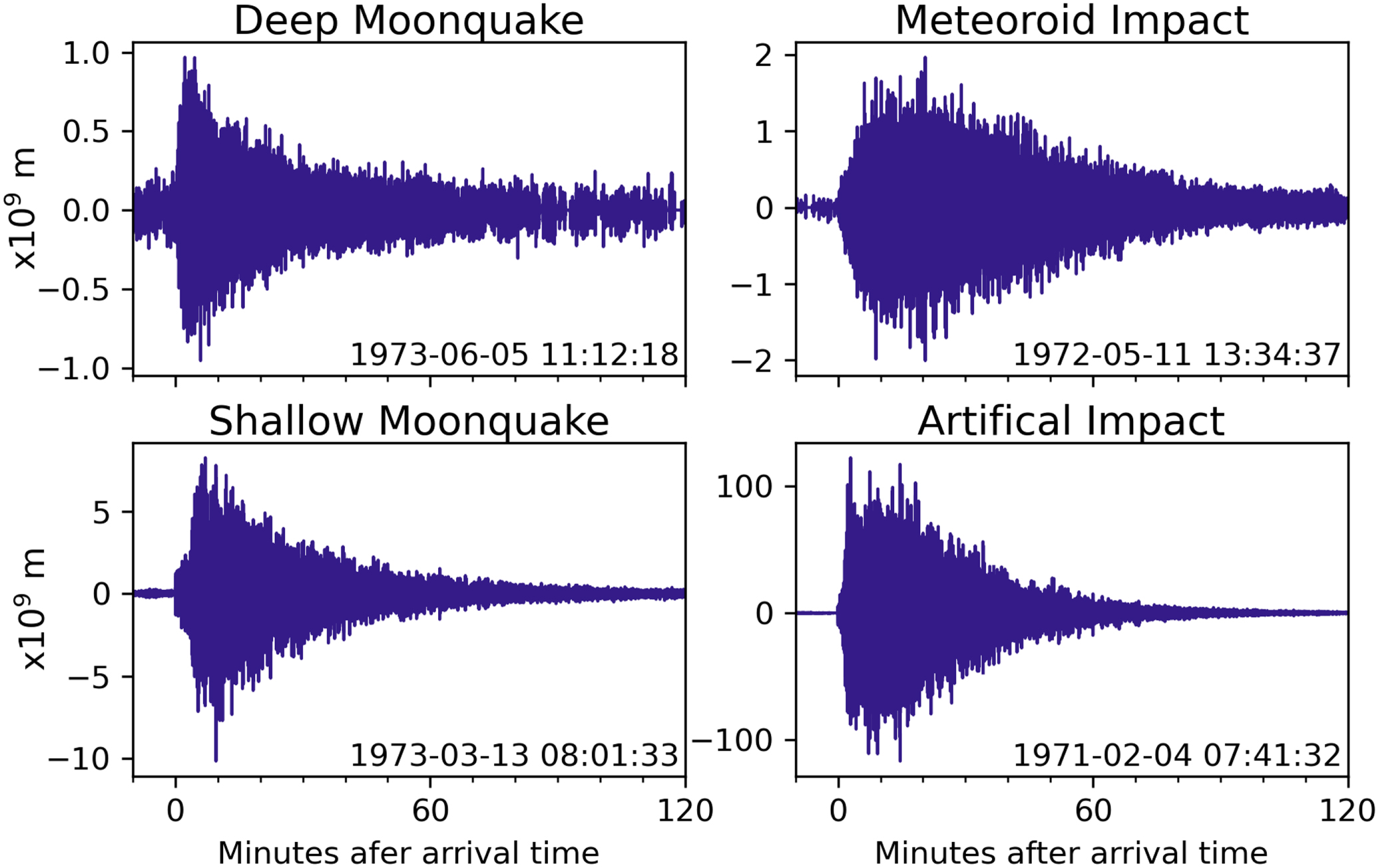
Standard image High-resolution imageThe analysis of the seismic data from the Moon yielded many surprises. Figure 3 shows the different types of lunar events. Deep moonquakes, located to depths of 700–1200 km (Nakamura et al. 1982; Nakamura 2005), were probably the most surprising. The peaks in deep moonquake activity had a periodicity of ∼27 days. Consequently, researchers associated the quakes with tides acting on the Moon (Lammlein et al. 1974; Lammlein 1977; Nakamura 2005).
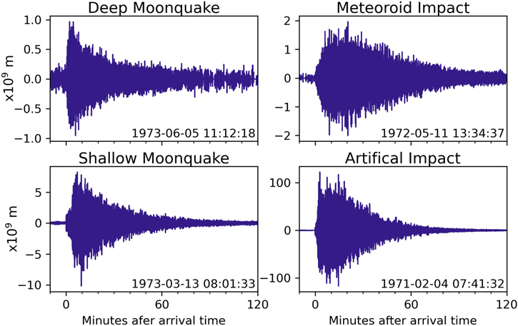
Figure 3. Examples of a deep moonquake, a meteoroid impact, a shallow moonquake, and an artificial impact. The events were recorded on seismic station S12 on the vertical component (MHZ). The timing for each event is in minutes and relative to the arrival time. The traces are displayed in displacement (in meters), with different scales for each event. The amplitude of the artificial impact signal exceeded the range of the instrument.
Download figure:
Standard image High-resolution imageShallow moonquakes, with possible depths between 50 and 220 km (Khan et al. 2000) and estimated equivalent body wave magnitudes of 3.6–5.8 (Oberst 1987), were also surprising. They may have a tectonic origin, since they are similar to intraplate quakes on Earth (Nakamura 1980). Figure 3 also shows examples of meteoroid strikes and artificial impacts.
The characteristics of the signals were also surprising when compared with terrestrial seismograms. Events of all types show long slow rise times and very slow decay of energy. The energy is strongly scattered, consistent with a highly fractured environment, especially near the surface. Even quite small events can last for 1 h, and the largest recorded event lasted for 5 h, which requires very low attenuation compared to Earth. In total, Nakamura et al. (1981, updated 2018) cataloged over 12,000 events recorded on the mid-period seismometers (the catalog is available in Nakamura (1981) and Nunn et al. (2020, Electronic Supplement)).
Although seismic phases associated with the lunar core are challenging to see, recent work using stacked traces has indicated a small lunar core (∼330–420 km in radius; Garcia et al. 2011; Weber et al. 2011). Recent observations from the GRAIL gravity mission have suggested an average crustal porosity of 12%, which is higher than previous estimates, and consistent with a highly fractured crust (Wieczorek et al. 2013). Using the higher estimates of porosities, the team modeled the average crustal thickness to be 34–43 km.
Various space agencies are planning future lunar missions, including seismic missions. NASA's Farside Seismic Suite, which is due to fly in the mid-2020s, would visit Schrödinger Crater. One of its mission objectives is to determine whether the Moon's farside is as seismically active as the nearside (Panning et al. 2022). The Lunar Geophysical Network is currently in formulation for NASA's New Frontiers 5 Announcement of Opportunity (Neal et al. 2020). The mission would contain a network of seismometers and geophysical instruments spread around the Moon at up to four landing sites. Existing observations from the Apollo network will continue to be useful to compare with these future missions.
This project to archive the data in SEED (Standard for the Exchange of Earthquake Data) format initially began with another project, which required an accurate understanding of the relative timing between data samples taken at the different Apollo stations. However, a clear sense of the timing was difficult with the available data. A version of the Apollo data, extracted to SEED format by researchers at the Institut de Physique du Globe de Paris, was formerly available at the Incorporated Research Institutions for Seismology (IRIS), but has been removed because the data users found serious timing inconsistencies. Apollo data were also available from the Japanese Aerospace Exploration Agency (JAXA), which included timing information. In this version, each record had been extracted to a database. This version did not correct for the timing inconsistencies already present in the original tapes. Additionally, the timing errors were difficult to rectify. Since the data were recorded in real time, the original tapes were sequential, so if they contained timing errors, the errors were easy to spot and sometimes possible to rectify. However, in the database version, if the timing was incorrect, the record was out of sequence, making it difficult to correct the timing. To deal with these errors, we reextracted the data from copies of the tapes provided by JAXA and made corrections to the timing. We processed the data into the widely used SEED format, and we decided to share the new archive with other users.
There are two major obstacles to formatting the data in a modern format. The first problem is that the data have slightly varying sampling rates, mainly due to the sensitivity of the data sampler to the significant temperature variations on the Moon's surface. The second problem is that the timestamp records when the signal arrived on Earth, rather than when the instrument took the measurement. This problem introduces a delay and adds an additional time variation relating to the rotation of the Earth, the libration of the Moon, and the Moon–Earth distance. Modern formats, such as SEED, require constant sampling rates. We solve this problem with a compromise. We give the data a constant sampling interval (the mid-period and short-period data have nominal sampling intervals of 0.150 943 4 s and 0.018 867 9 s, respectively). However, we retain a separate track that contains the timestamps. We see a slight positive or negative drift of a few seconds after 24 h, which is different for different stations. The time track contains information about the actual sampling interval at any given time. We provide the data in the original raw format, so that users can control the data processing that they apply.
We begin this paper with a description of the Apollo seismometers. Next, we describe the steps to extract the data. We follow with a description of the data in the new archive. We end with a summary of how to access the archive.
2. Description of the Apollo Seismometers
Our data archive covers the passive experiments, which included mid-period and short-period instruments. The mid-period seismometer contained three matched sensors, aligned orthogonally to measure one vertical (MHZ) and two horizontal components (MH1, MH2) of surface motion, and the short-period instrument contained a vertical sensor (SHZ). Note that we use the current naming conventions. In many earlier papers, the mid-period seismometers were called the long-period seismometers, and the channels were named LPX, LPY, LPZ, and SPZ (these correspond directly to MH1, MH2, MHZ, and SHZ).
Here, we provide a brief description of the seismometers (see Nunn et al. 2020 for more information). The mid-period seismometer made measurements proportional to displacement, unlike most modern seismometers covering these frequencies, which make measurements proportional to velocity. The nominal sampling interval was 0.150 943 4 s.
The instrument could operate in one of two modes: peaked-response or flat-response. Figure 4 shows the transfer functions for the two modes. In peaked-response mode, the transfer function was sharply peaked at 2.2 s. The seismometer acted as an underdamped pendulum (Latham et al. 1973). The engineers also designed a flat mode, to be sensitive to a broader range of frequencies, and used a positive feedback filter in the circuit. In the flat-response mode, the seismometers had natural periods of 15 s and could detect ground motions as small as 0.3 nm over the frequency range from 0.1 to 1 Hz (Latham et al. 1973). The maximum sensitivity in the peaked mode was 5.6 times greater than that in the flat mode, but the low-frequency sensitivity was reduced (Latham et al. 1973). Unfortunately, the flat mode was not very stable, and the seismometers were mainly commanded to operate in peaked mode. Figure 2 shows the times when the seismometer operated in peaked or flat mode.
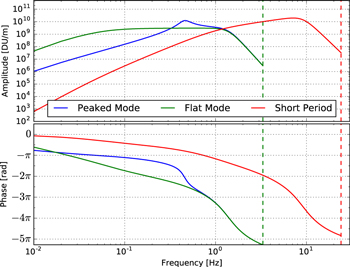
Figure 4. Transfer functions. Displacement amplitude (top) and phase (bottom) transfer functions for the flat and peaked modes of the mid-period seismometer and the short-period seismometer. The plots show the nominal responses up to the Nyquist frequency (dashed lines). The units of amplitude are the DUs per meter. The phases show the counterclockwise angle from the positive real axis on the complex plane in radians. The transfer functions in velocity and acceleration are available in Nunn et al. (2020).
Download figure:
Standard image High-resolution imageThe short-period sensor was a vertical sensor with a standard coil magnet velocity transducer. It had a displacement response peaked at approximately 8 Hz (Figure 4), and the nominal sampling interval was 0.018 867 9 s.
3. Importing to SEED Format
In this section, we describe how the data were recorded, and the processing required to archive the data in SEED format.
3.1. Data Recording and Preservation
The data were digitized on the Moon, transmitted in real time, and recorded at one of the Deep Space Network ground stations. The data were recorded on an analog tape, known as a range tape, in pulse-coded modulation, a type of frequency modulation. Standard time was recorded on a separate track. The ground stations were spaced around the Earth, and at least three stations would operate over 24 h, to maintain a good line of sight to the Moon. Often, during the transition from one station to another, there was a brief overlap where two stations were recording simultaneously, although gaps were also common.
Until the end of 1976 February, the range tapes were sent to the Manned Spacecraft Center (now the Johnson Space Center, or JSC). At JSC, the data and the standard timestamp recorded on the range tapes were read, and the data relevant to each experiment were recorded on 7-track reel-to-reel digital tapes, called PI tapes, with timestamps corresponding to the beginning of each frame.
From the beginning of 1976 March, the range tapes were sent to Galveston Geophysics Laboratory, at the University of Texas Medical Branch, and the full data on the range tapes were read and recorded on 9-track reel-to-reel digital tapes, called work tapes, with timestamps corresponding to the beginning of each frame.
In the early 1990s, as significantly higher-capacity digital recording media became available, the data from all the passive seismic experiment PI tapes (7200 7-track tapes) and work tapes (1486 9-track tapes), together with other tapes, such as the passive seismic experiment event tapes and tapes from the Viking project, were reformatted and copied to 80 exabyte cassette tapes (Nakamura 1992). Copies of these cassette tapes were sent to the Institute of Space and Astronautical Science, now a part of JAXA, which funded the tape copying process, and to IRIS, for archiving. Copies of the exabyte tapes are available from IRIS, the NASA Space Science Data Coordinated Archive (NSSDCA 1992, Dataset ID: PSPG-00739) and JAXA (JAXA 2012).
The user should be aware that there have been many steps in preserving and sharing these data. At each step, including the latest, which we outline below, there were possibilities of errors being introduced or data being lost.
3.2. Step 1—Extracting the Data from the Tape Copies
We extracted the binary data from digital copies of the exabyte tapes using the data schema described in Nakamura (1992). The data sampler on the Moon recorded the data in blocks (physical records) of 90 frames each. Within each frame, the data were arranged into 64 10-bit ALSEP words, evenly spaced in time. Each frame is equivalent to around 0.603 77 s (64 words per frame, 10 bits per word, and a sample rate of 1060 bits per second), and each block of 90 frames has a length of around 54.3 s. Each component of the mid-period seismometers (MH1, MH2, and MHZ) recorded four samples per frame. SHZ used the even words within the block, except for words 2, 46, and 56, which were reserved for other tasks. Additionally, word 24 on S15 was reserved for another experiment. Thus, the SHZ timing is evenly spaced, but with three or four missing data samples per frame. The nominal sampling interval is 16/106 s or 0.150 943 4 s for the mid-period instruments and 2/106 s or 0.018 867 9 s for the short-period instruments.
3.3. Step 2—Error Checking
We checked the extracted data for errors, beginning with checking the Barker code. The transmission contained a Barker code, which is a code with a series of zeros and ones in a preset pattern. An intact Barker code indicates that the receiver has read the transmission correctly. The traces show that when the Barker code was incorrect, the corresponding data samples were meaningless. We rejected all data with damaged Barker codes (approximately 0.3% of all the available data). We also examined the traces to determine whether we could extract data from a damaged trace (for example, by shifting the zeros and ones to find a match to the Barker code). However, this did not seem possible. Transmission errors usually occurred in blocks. The blocks could begin or end at any point in the frame, and affect all data between the endpoints. Damaged traces could run consecutively for minutes or hours or be more sporadic. Our despiking algorithm (see Step 3 below) includes code to deal with this problem of frames that are partially damaged.
The data were recorded alongside a frame number, which ranges from 0 to 89. The frame was recorded by the sampler and transmitted with the data. This number helps to correctly determine when traces overlap (due to recording at two ground stations). When the reel-to-reel tape recorder could not read the data correctly from the range tape, it often inserted a second or third frame with the same frame number. A repeated frame number with timestamps close to each other indicates this problem. It is clear that these are repeated frames, rather than extra ones, because the frame number is the same and the subsequent frame has the correct frame number and approximately the correct timing. We found cases where the sampler reset the frame number to zero before finishing the previous physical record, although these cases are not particularly common.
When two ground stations received data simultaneously, the timestamps did not match exactly. We expect slight timestamp differences, because the lines of sight from the seismic station on the Moon to the two different ground stations were not the same. Additionally, the distances from the standard time transmitter to each of the ground stations were not the same. These systematic time differences are in addition to errors caused by unsynchronized reference clocks at the stations or difficulties in reading the clocks. We take advantage of the fact that the data are transmitted in real time to test for errors in the transmission. For example, the timestamp is probably incorrect if it suddenly jumps forward or backward in time. The binary data could be damaged either during transmission or later, as the tapes deteriorated. Therefore, flipped bits could damage the timestamp, the frame number, the station code, the ground station, or the sensor data.
Although the data did not have constant sampling intervals, most sample intervals fell within a narrow range. A nominal frame is 0.603 773 584 9 s. Nearly all sample intervals are either 0.603 s or 0.604 s (we expect this because the precision of the timestamp is only 0.001 s). We made the following corrections to the data. We amended single frame numbers that were out of sequence but had the correct timestamps. We also amended single timestamps that were out of series but had the correct frame numbers. Next, we determined the sections of traces with "good" records—those that had a single increment of the frame number and that had a timing gap greater than 0.600 9 s and smaller than 0.607 s (that is, close to the nominal frame interval of 0.603 773 584 9 s). We checked for blocks of these consecutive "good" records. We tried to amend the timestamps by using the last record of a consecutive block and the first record of the next consecutive block. Where there were data gaps, we inserted the correct number of empty samples between frames (using a combination of the time and the frame gap). We ignored small errors in the sampling interval at this stage. Finally, we dropped any remaining records that were in sections that did not contain at least 180 consecutive frames of good records.
To reduce the timing errors, we kept only the sections of traces with at least 180 consecutive frames (∼109 s). These sections may contain gaps in the sampling, but we require interpolated timestamps and frame numbers that fit the correct number of frames and the sampling interval. This precaution prevents random timing errors and allows us to use an algorithm to check the entire mission for timing errors. Unfortunately, our approach sometimes excludes potentially valid data when the sampler was running particularly fast or slow. We relaxed the criterion of at least 180 consecutive frames to 10 frames, when we found that the original algorithm had missed some valid data for some large events. We then checked these imports manually.
The time when the signal arrived on Earth was usually determined by a standard time signal received at the ground station. However, when the computer could not read the standard time signals recorded on the range tapes, it would generate a timestamp (Nakamura 2011; Knapmeyer-Endrun & Hammer 2015, supplement). The "software clock" could lead to offsets of more than 1 minute, in comparison with the standard time (Nakamura 2011). From 1973, a flag was set by the data processor at JSC to indicate the use of the software clock. When the flag was set, we corrected the timestamps by interpolation, resulting in no offsets.
The operators noticed that the MHZ component of S14 was inoperative on 1972 March 20, and concluded that the problem was either a component failure or a wire connection problem. The problem was eventually resolved on 1976 November 17, when the z-axis responded to leveling. Additionally, we noticed several issues in the days leading up to the initial error. We therefore exclude data from the MHZ component on S14 from 1972-03-12T00:00 to 1976-11-17T00:00. Similarly, the SPZ component of S12 was inoperative throughout the mission.
In the tape copies, we found examples of data being attributed to the wrong station. For example, we found a section of the traces being swapped from S12 to S15 within the tape from approximately 19:47 on 1976-04-01 to 03:25 the following day (a figure is included on the GitHub site). When viewing the copied traces, we find a section of the MHZ trace on S12 that jumps from being centered around 526 digital units (DU) to one centered around 505 DU. We see the opposite change on the S15 trace. We also found a second error type, where the data from one station were copied to another station. Both errors were usually only a few minutes in duration. We systematically searched for the copies and excluded these sections. We also looked for swapped data, although we cannot be certain that we have found all the swapped sections. If we have missed any affected traces, then the symptoms of this problem would be discontinuous jumps in the centerline or sudden changes in the noise profile. We swapped the data from 1976 April 1 and 1976 April 2 back to the correct stations, and excluded the other short sections that we found.
3.4. Step 3—Making the MiniSEED Files
In the final step, we make miniSEED files from the cleaned data. MiniSEED files are the subset of the SEED format for time-series data. Where possible, we try to construct traces with continuous sampling. Although these traces may contain missing samples, the timing trace is continuous. As explained in the previous section, we use the frame numbers combined with the timestamps to determine where these gaps should be.
When constructing the miniSEED files, there is a sample time and a timestamp time. The sample time is based on the nominal sampling interval and the number of samples. The timestamp is based on the time when the sample was received on Earth. To estimate the start time of any trace, we estimate the number of samples since midnight using the actual sampling interval. We can then calculate the sample time using the nominal sampling interval. At midnight, these times are the same, but they diverge during the day.
To construct the continuous trace, we check for an overlap and try to match the frame number. A perfect match has the same frame numbers and data in the old and new traces. If we can match the frame number, we set the start time of the new trace at this time. If we cannot match the frame number in the overlapped trace, this is an error with either the new or old trace. We start the new trace at the new time and record an error in the log. If there is no overlap, we try to fit a gap with the exact number of frames between the end of the previous trace and the beginning of the following trace. If matched, we start the new trace at the correct time to take account of the gaps. If we cannot fit an exact gap, we estimate the start time of the sample.
The output miniSEED file is a one-day record from a few milliseconds after midnight until the following night. Note that the trace will not finish at exactly midnight, because we reconstruct a continuous trace with a nominal sampling rate that does not precisely match the actual sampling rate (which will also vary during the day). Data samples may overrun into the next day (rarely by more than ∼6 s). When using the automatic download from IRIS, the data that overrun into the next day are truncated. The full one-day records, including the overruns, can be accessed at the Planetary Data System.
We run a despiking algorithm on the trace (Figure 5). We designed the algorithm to remove single digital spikes only. These occur when a single data point is incorrectly recorded (probably caused by a flipped bit during transmission). We remove these spikes at this stage because they are relatively easy to remove and are not related to the function of the seismometer. Figure 6 shows the process of data cleaning. The top trace shows the original data. The bottom trace shows the data imported, excluding the data damaged in transmission (we excluded data if the Barker code was incorrect). The bottom trace has also been despiked.
We felt that entirely excluding the damaged data (as identified by the incorrect Barker codes) was the best solution. The sequence of digits is meaningless unless their positions are known. As the Figure 6 shows, the start of the event is contaminated by high values, and the end is contaminated by both high and low values. Often, the data nearer to the average also become erratic, although these are harder to see. Removing the damaged data can make traces clearer and make it possible to interpolate across the damaged sections.

Figure 5. Digital spike removal. The top panel shows test data with added digital spikes, while the bottom panel shows the data after the spike removal process. The algorithm removes single spikes, spikes before a gap, and spikes after a gap. Up and down spikes and double spikes (which have two data points within the spikes) are not removed by the algorithm.
Download figure:
Standard image High-resolution image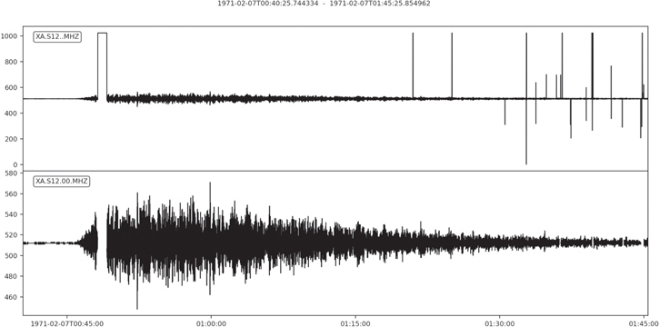
Figure 6. Data cleaning. The top panel shows the original data imported from the tape. The bottom panel shows the same data reimported, but excluding data with incorrect Barker codes (incorrect Barker codes indicate data frames that were not transmitted correctly). We have also removed single digital spikes from the trace (Figure 5 shows examples of these spikes).
Download figure:
Standard image High-resolution imageFinally, we made some corrections to the timing errors. The "software clock", described above, introduced errors of several seconds to the timing of the traces. After 1973, the error was flagged, but the error was present from the start of the mission. We searched for the affected sections, marked the sections of the timing traces to be interpolated, and corrected the timing, where possible.
There was a second problem, mainly affecting the work tapes, which we correct for. There was a tape head wiring error that caused a shift in the recording data streams for some stations, resulting in a time shift of either 400 or 800 ms, at some range stations at some times. We add 400 or 800 ms to the timestamps during this step. We also corrected for some systematic offsets of 1 or 2 s that occurred occasionally throughout the mission.
Third, we found some some sections where we are unable to reconstruct the timing correctly, where the timing trace is too fast or slow. There are also some sections that may have missing or extra data samples. This is probably related to the data sampler occasionally resetting itself to zero during the middle of a record (normally 90 frames per record). Although we dealt with this problem on continuous traces, it was not possible to deal with it on traces with gaps. The GitHub site includes logs of the timing corrections (TimeErrorIntervals.csv) and the sections that we flagged with potential errors and visual representations of the timing before and after our corrections.
4. Description of the Archived Data
This section describes how to understand the data. We provide five tracks of data (Figure 7): three components on the mid-period seismometers (MH1, MH2, and MHZ), the short-period sensor (SHZ), and a timing trace, ATT. Each data track is in raw format. We name the mid-period channels MH1, MH2, and MHZ, to be consistent with the IRIS naming conventions. The "M" reflects the mid-period data and a sampling rate between 1 and 10 Hz. The "H" is for a high-gain seismometer. Finally, since the horizontal channels do not always point north or east, we use 1 and 2 to indicate the channel orientations. The correct orientations are in the metadata. The mid-period seismometers ran in either flat or peaked mode. We split the files into locations "00" for the peaked mode and "01" for the flat mode. The location field is blank for SHZ and the timing trace ATT.

Figure 7. Data tracks provided in the miniSEED files. The top four traces show the components MHZ, MH1, MH2, and SHZ. The x-axis is the time in seconds after the P-arrival (1971-02-07 00:45:45) and the y-axis is in DU. The fifth trace, ATT, shows the timestamp. The y-axis is the number of seconds since 1970 January 1 (it is displayed with an offset of 34735545.6 s between 1970 January 1 and the arrival time).
Download figure:
Standard image High-resolution imageAs described above, there are missing samples for the SHZ traces. We substitute a value of –1 for each of these missing values on the traces. We also do this for the missing samples on the mid-period traces. The traditional approach to missing samples is to mask the traces in the miniSEED file. However, we found that the missing samples were so frequent that the data files were significantly larger and there were performance issues when using this traditional approach. We stress that users should read the traces and replace the –1 values with masks or interpolate the data. There is a code snippet on our GitHub repository to do this. 4 Users may also find it helpful to remove glitches before beginning their analysis, since our despiking algorithm removes only single digital spikes.
The ATT tracks contain the timestamp, measured in seconds from 1970 January 1 (the timestamps from 1969 are negative). The time can easily be recovered with ObsPy (Beyreuther et al. 2010), using the class UTCDateTime (e.g., the command UTCDateTime(-14182916.0) will recover 1969-07-20T20:18:04.000000Z). Note that the original data recorded on the tapes used a different convention for the timestamps. The sampling interval for the timing trace is 0.603 773 584 9 s, because the timing was recorded once per frame. When the ground station changes, the timing trace takes the timestamp from the new station.
The data were recorded with DU, with values from 0 to 1023. The values lay somewhere in the middle of the range when the seismometer was at rest, although the rest position varies with the time of lunar day. One DU corresponded to ∼0.08 nm of ground displacement in the peaked-response mode and ∼0.3 nm in the flat-response mode at 0.45 Hz. Users can transform the data into displacement, velocity, or acceleration with the provided metadata files.
The samples for each of the mid-period sensors were not taken simultaneously, which has implications when comparing the signals of the three components. The first MH1 sample (ALSEP word 9) was sampled 10/1060*8 = 0.075 s after the head of the frame. MH2 and MHZ were sampled 0.094 and 0.113 s after the head of the frame, respectively. SHZ is sampled at every even position and so begins at 10/1060 = 0.009 s after the head of the frame (note that the first position was blank, but is included in the timing). We provide the MH1, MH2, MHZ, and SHZ traces with time shifts of 0.075, 0.094, 0.113, and 0.009 s relative to the ATT traces. Particular care should be taken when considering wave polarization. Additionally, users should note the orientations of the horizontal components, which are available in the metadata.
We constructed the miniSEED files with a nominal sampling rate. There can be a positive or negative time shift of up to a few seconds after 24 h, as shown in Figure 8. In many situations, data users may find removing the drift necessary, by using the information provided on the timing trace ATT.
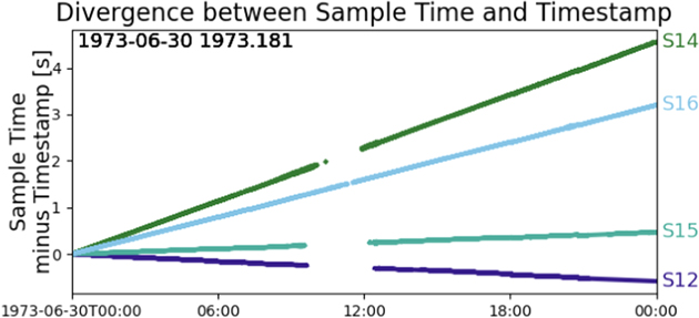
Figure 8. Divergence between sample time and timestamp. Each of the data samplers controlling the sampling on the seismometers had a slightly different sampling rate that varied over time. As far as possible, the data are provided as continuous traces. Therefore, there is some divergence between the time estimates from the continuous sampling and the recorded timestamps. Data users should be aware of these differences and may need to correct for them. The divergence lines are curved. Additionally, the traces show some gaps where data were not recovered due to timing issues.
Download figure:
Standard image High-resolution imageWe chose a single nominal sampling rate for all stations for all days. Although we could have defined a rate for each station, the rate for each station varied considerably over the course of the mission. Therefore, there was no obvious choice for any one station. On average, the sampling rate was slightly lower than the nominal rate. Considering that there was no obvious choice for each station, we decided to have all stations use the same rate.
There is a 1.2–1.4 s delay time when transmitting from the Moon to Earth, which we do not correct for. Additionally, we do not correct for the apparent variations in the sampling rate that are caused by changes in the orbital parameters of the Moon–Earth system, such as by the rotation of the Earth, the libration of the Moon, or changes in the Moon–Earth distance.
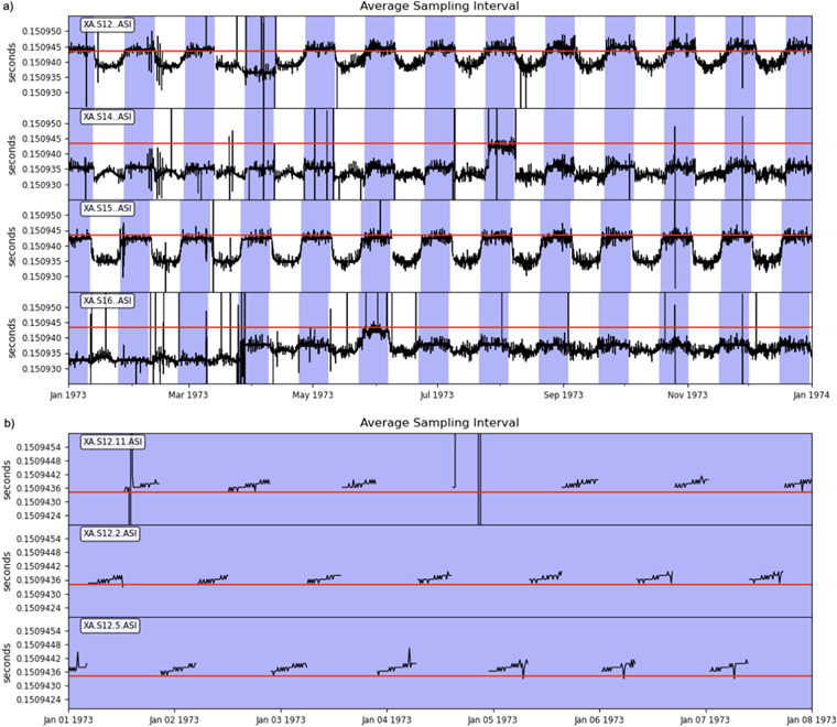
The sampling interval was strongly dependent on whether it was lunar day or night (Figure 9(a)). Sampling was reasonably constant during lunar night, but strong variations occurred during the day, especially at sunrise and sunset. This variation was probably caused by strong temperature fluctuations on the lunar surface. This was because the oscillator that controlled the sampling was not temperature-compensated. In addition, there were short-term fluctuations in the sampling interval. The rotation of the Earth also had a small effect on the apparent sampling interval (Figure 9(b)).
Figure 9. Variation in the sampling interval. (a) The variability of the sampling interval for each of the stations during 1973. (b) The variability of the sampling interval from 1973 January 1 to 7 for station S12, recorded at different ground stations (02: Ascension Island; 05: Guam; 11: Corpus Christi, Texas). The rotation of the Earth has a small effect on the apparent sampling rate (it does not affect the real sampling rate). The increase in the apparent sampling rate while a ground station is recording on (b) is due to the rotation of the Earth. The apparent sampling rate is lower when a new ground station starts recording. In both plots, we averaged the sampling over approximately 15 minutes. The plots show alternating periods of lunar night (purple) and lunar day (white). The red lines show the nominal sampling interval (0.1509434 s).
Download figure:
Standard image High-resolution image
There are therefore many errors associated with the timing: the variability of the sampling on the Moon, reception errors, recording errors, the distance from the source of the standard time signal to the ground station, and the variation introduced by the rotation of the Earth, the libration of the Moon, and the distance from the Moon to the Earth. Only the first of these errors affected the actual sampling rate. The others only affect the apparent sampling rate. Therefore, the recorded sampling interval is only a guide to the actual sampling interval.
The team were able to send commands to the seismometers. The commands included options to change the seismometer gain, to send calibration pulses, and to change the mode of the mid-period seismometer from flat to peaked, or vice versa. The timing of these commands is included in our GitHub site, along with an example calibration pulse. 5
We provide the nominal instrument responses in the metadata files. Horvath (1979) evaluated the differences between the nominal transfer functions provided by the engineers (and provided within the response files) and the actual transfer functions. The actual transfer functions had some differences between the stations and over the lifetime of the instruments. The team sent calibration pulses to the seismometers. A step of current equivalent to a known step of ground acceleration was applied to the coil for each of the seismometer components (Latham et al. 1973). Additionally, the engineers controlled the gain from Earth, and were able to cycle through the options (from maximum gain, −10 dB, −20 dB, −30 dB, and back to maximum). The timing of the gain commands is known, and provided on our GitHub site, but the resulting gain can only be found by checking the seismograms. 6 The metadata files use the highest gain, but there are periods when lower gain was used. In general, the seismometers operated at maximum gain.
We provide a Getting Started notebook on our GitHub site. 7 The notebook includes some example seismograms, with the instrument response removed. It also provides code to view and correct the timing divergence.
5. Data Archive
The data described within this paper are archived at IRIS with the following DOI:10.7914/SN/XA_1969.
We have archived the data on the Geosciences Node at the Planetary Data System. 8 Table 1 shows the percentage of data recovered and placed into the archive.
Table 1. Data Recovery
| Data Recovery | |
|---|---|
| Valid Records | 96.5% |
| Not Recovered (Damaged Records) | 0.3% |
| Not Recovered (Timing Issues) | 1.1% |
| Not Recorded | 2.0% |
Note. For the duration of the mission at stations S12, S14, S15, and S16, the percentages of valid records, records that were damaged during transmission, records that were not recovered by us due to timing issues, and records that were not recorded by the mission. Note that periods of time when the seismometers were transmitting data but not sending back valid seismic records are not excluded from the estimation of valid records.
Download table as: ASCIITypeset image
6. Data and Resources
Our GitHub repository includes the following additional information: the locations of the seismic stations; the operational status of the instruments (originally from Bates et al. 1979); the timing of the commands sent to the instruments; the times when the mid-period seismometers were operating in flat mode; the codes for the ground stations receiving the signals; and example calibration pulses. 9
If use is made of this work, authors should cite Latham et al. (1970), and Yamada et al. (2012), as well as this paper.
We used ObsPy extensively during this project (Beyreuther et al. 2010). Figures have been produced with the Python tool Matplotlib (Hunter 2007). Figure 1 was produced with Cartopy (Met Office 2010), using topographic data from Araki et al.(2009).
This work was finalized with a grant from the National Aeronautics and Space Administration's Planetary Data Archiving, Restoration, and Tools (PDART), proposal No. 19-PDART19_2-0052, task No. 811 073.02.37.01.99, and also supported with strategic funds from the Jet Propulsion Laboratory, California Institute of Technology, under a contract with the National Aeronautics and Space Administration. The work was initially funded with the European Union's Horizon 2020 research and innovation program, under the Marie Skłodowska-Curie grant agreement No. 659773. This work benefited from discussions at the workshop "An International Reference for Seismological Data Sets and Internal Structure Models of the Moon" supported by the International Space Science Institute in Bern, Switzerland. The authors would like to thank the editor, Dr. Edgard G. Rivera-Valentín, and two anonymous reviewers for their helpful comments, which led to improvements to the manuscript.
© 2022. All rights reserved.
Software: ObsPy (Beyreuther et al. 2010; Megies et al. 2011); Matplotlib (Hunter 2007).
Footnotes
- 4
- 5
- 6
- 7
- 8
- 9