


Abstract
Quantifying the volumes and geologic nature of lunar volcanic eruptions is important for constraining the thermal and geologic evolution of the Moon. Cryptomaria are effusive, basaltic lava flows on the Moon that were subsequently buried, and therefore hidden, by higher-albedo basin and crater ejecta. Radar offers the ability to probe the subsurface for geologic units not otherwise apparent at the surface. We use Arecibo/Green Bank Observatory and Lunar Reconnaissance Orbiter Mini-RF radar data sets to characterize maria and cryptomaria within the Schiller–Schickard region. We find significant variability in the radar backscatter across the region that does not correspond to previously mapped boundaries of maria and cryptomaria in the literature. We use the characteristic low backscatter (due to the attenuating nature in radio waves of some basaltic minerals) to analyze the distribution of cryptomaria. We use the reduction in radar backscatter to estimate burial depths of cryptomaria across the area. We present a new map of Schiller–Schickard cryptomaria and the local variability in the thicknesses of the light plains that bury the basalts. We find burial depths ranging from >100 m in the deepest areas to just a few to tens of meters in areas with shallow cryptomaria (particularly prominent in the southeast). These areas are generally contiguous with maria, allowing us to track mare lava flow units into the subsurface at mare/highland margins. We propose that ∼67% of the region contains surface or buried basaltic volcanism, which represents over twice (2.7× increase) the areal extent of cryptomaria reported in previous studies.
Export citation and abstract BibTeX RIS

Original content from this work may be used under the terms of the Creative Commons Attribution 4.0 licence. Any further distribution of this work must maintain attribution to the author(s) and the title of the work, journal citation and DOI.
1. Introduction
Maria are low-albedo and effusive basaltic lava flows concentrated on the nearside of the Moon (e.g., Head 1976). Cryptomaria (cryptomare in the singular) are a subset of these lava flows that were emplaced early in lunar history and have been subsequently buried by higher-albedo basin/crater ejecta (e.g., Head & Wilson 1992; Antonenko et al. 1995). Thus, cryptomare deposits are an enigmatic and often invisible portion of the lunar upper crust, being veiled by generally unknown periods of lunar history and corresponding stratigraphy. Understanding the distribution of cryptomaria, therefore, provides crucial information toward a more complete understanding of the spatial and temporal history of volcanism on the Moon.
Cryptomaria have been identified in a variety of ways, but perhaps most common is through the presence of dark-halo craters (DHCs) in visible images (Bell & Hawke 1984; Antonenko et al. 1995). DHCs (which are distinct from radar-dark halos; Ghent et al. 2005) have a characteristic ring of low-albedo ejecta that consist of materials from the dark, subsurface basalts excavated by these small (<10 km) craters. These dark basalts are thought to underlie the higher-albedo surface materials at depths of meters to hundreds of meters (e.g., Schultz & Spudis 1983; Bell & Hawke 1984). Additional criteria, such as spectral mixing and geochemical analyses of the composition of surface materials to look for basaltic signatures in the regolith, as well as proximity to maria, are also used in the identification of cryptomaria (e.g., Antonenko et al. 1995). Maxwell & Andre (1981) argued that mass concentrations observed in gravity data may identify candidate cryptomaria regions as well, and Sori et al. (2016) used data from the Gravity Recovery and Interior Laboratory (GRAIL) mission (Zuber et al. 2013) to find positive Bouguer gravity anomalies coincident with proposed cryptomaria along an arc in the southern lunar nearside extending across Schiller–Schickard, Maurolycus, and Mare Austale, as well as in the Lomonosov–Fleming region on the farside.
The light plains materials that bury the cryptomaria are higher-albedo (compared to the mare), relatively smooth ejecta material generated from basin-forming (and other impact) events, impact melt deposits, and perhaps non-mare volcanism in the case of the Apennine Bench Formation (Meyer et al. 2020). Whitten & Head (2015a) combined a variety of imaging, spectral, thermal, and altimetry data sets to investigate and characterize 25 locations previously proposed to be cryptomaria. They argued that 20 of these 25 locations contain cryptomaria using color composite data in the visible to near-infrared from the Moon Mineralogy Mapper (M3) instrument on board Chandrayaan-1 to search for pyroxene bands at 1 and 2 mm within DHCs in order to find those that excavated basalt. Cryptomare sites were confirmed and mapped based on the distribution of the DHCs and extent of the pyroxene-rich regolith. Based upon visible images from the Lunar Reconnaissance Orbiter Camera (LROC) and topography from the Lunar Orbiter Laser Altimeter (LOLA), they refined the areal boundaries of the cryptomare at each site to include contiguous areas of the same morphology (surface texture, albedo, and elevation) as the pyroxene and DHC-rich terrain. After mapping boundaries associated with each cryptomare unit, they characterized the topography, surface roughness, rock abundance, albedo, and geologic/geographic relationships to craters for each site. Whitten & Head (2015a) concluded that mapped cryptomaria and non-cryptomare light plains could not be distinguished from each other on the basis of those properties, although they predicted that the basin ejecta distributions and stratigraphy of 27 lunar impact basins could contribute to light plains thicknesses of 27–247 m. The cryptomare regions they mapped cover a total of ∼2% of the Moon, which increased the known extent of the lunar surface that mare volcanism has been emplaced upon (either through exposed surface mare or cryptomare) to ∼18% (Whitten & Head 2015a).
Radar wavelengths that have been utilized to observe the Moon to this point offer the ability to probe the near subsurface on decimeter to decameter scales, which can therefore be used to look for previously unknown cryptomare deposits that may either be (a) too deep to have been incorporated into surface materials characterizable by spectral signatures, (b) not at the depths or locations exposed by impact craters (e.g., DHCs), and/or (c) too small or of insufficient mass to be detectable by GRAIL gravity data. The composition of the basalt strongly affects the radar signal, and ilmenite (an iron titanium oxide mineral, FeTiO3), in particular, affects the bulk loss tangent, leading to greater attenuation of the radar signal (e.g., Carrier et al. 1991; Campbell et al. 2014). Campbell & Hawke (2005) observed a decline in radar backscatter with increasing TiO2 and FeO abundances in regions sampled north and northwest of Schickard. These relationships between the composition and radar properties of lunar rocks and minerals have been leveraged to map the stratigraphy of volcanic flows within Mare Imbrium (e.g., Morgan et al. 2016). Knowledge of this phenomenon enabled Morgan et al. (2016) to determine that Mare Imbrium contains four major volcanic units that are comprised of 38 individual units (in this case, a stratigraphy of multiple mare units rather than maria buried by highlands ejecta/light plains). The 70 cm wavelength radar data from Arecibo Observatory (AO) and Green Bank Observatory (GBO) were also previously utilized by Campbell & Hawke (2005) to find and map cryptomaria east of Orientale basin (0°–45°S, 55°–105°W). Based upon the low radar scattering returns to GBO, Campbell & Hawke (2005) determined that these deposits extend into the subsurface beyond the mare boundary areas evident with multispectral observations of the lunar surface. Their results demonstrated that the region between Cruger and Oceanus Procellarum, as well as some patches west/northwest of Humorum basin, had also been flooded in lava flows (Campbell & Hawke 2005). These flows extend in the subsurface over an area of 178 × 103 km2 and were estimated to be buried by up to tens of meters of highlands ejecta material. This augmented the areal extent of known lunar mare basalts by 2.7% at the time of that study (Campbell & Hawke 2005).
Distinguishing light plains that are not overlying mare basalts from light plains that are atop maria (i.e., cryptomaria) is difficult, and ultimately, the main distinguishing features for regions of cryptomaria have been the presence of DHCs with spectral features indicative of greater mafic proportions. Here we build upon previous lunar volcanic studies of the Schiller–Schickard region by utilizing radar observations to discern areas of light plains obscuring cryptomaria (Figure 1). Schiller–Schickard is one of the most studied locations of cryptomaria, with previous studies utilizing a combination of spectral mixing analyses (e.g., Head et al. 1993; Blewett et al. 1995; Mustard & Head 1996; Hareyama et al. 2019), DHCs and their nearby geologic context (e.g., Schultz & Spudis 1983; Hawke et al. 1985; Whitten & Head 2015a, 2015b), and gravity signatures (Sori et al. 2016). We augment these studies by utilizing data from bistatic ground-based (AO and GBO) and monostatic orbital (Lunar Reconnaissance Orbiter Miniature Radio Frequency Instrument, LRO Mini-RF) radar observations to map mare units from surface exposure to within the subsurface (thus becoming "cryptomaria") based upon contiguous regions of low radar backscatter. We perform a regional analysis to estimate upper limits of the thicknesses of the overlying ejecta. We then use this information to propose our interpretation of the stratigraphy, with corresponding burial depths, across the Schiller–Schickard region.

Figure 1. Maps of the Schiller–Schickard region of interest. (a) Global mosaic from the LRO WAC, with the red box indicating the location of the study region (and spatial extent of Figures 1(b), 2, 3, 9, 10, and 12). (b) Schiller–Schickard region that we consider (30–60°S, 40–70°W) with previously mapped units from the literature. Amber units indicate surface mare as mapped by Nelson et al. (2014). Bold black lines outline the boundaries of cryptomaria as mapped by Whitten & Head (2015a). Areas of white with purple speckles (and with 50% transparency) indicate light plains materials as mapped by Meyer et al. (2020). Orientale is to the northwest. The base map is the LRO WAC global mosaic. White dashed boundaries with number labels indicate the five locations highlighted in Section 3.1 (Figures 4–8). The map is shown in a plate carrée cylindrical projection; for scale, the distance between 10° latitude grid lines is ∼300 km, and the distance between 10° longitude grid lines is ∼260 km at a latitude of 30°S and ∼150 km at a latitude of 60°S.
Download figure:
Standard image High-resolution image2. Methods
We primarily conduct our analyses using ground-based P-band (70 cm; 430 MHz) radar data of the Moon, which has complete data coverage across the Schiller–Schickard area (∼30–60°S, 40–70°W). We also inspected S-band (12.6 cm; 2380 MHz) radar data from ground-based and orbital spacecraft data sets, although there are gaps (i.e., gores) in these data across the region, so they were used primarily for local scale comparisons rather than regional analysis. The wavelength for the S-band data is a factor of ∼6 shorter than that of the P-band, so comparing these different data sets illuminates similarities and/or differences in the shallow subsurface structure (with the Pband able to penetrate deeper but being sensitive to larger materials and interfaces as compared to the S band).
Ground-based data sets (both P- and S-band) were collected by transmitting a circularly polarized signal from the 305 m diameter dish of AO in Puerto Rico and receiving the lunar echoes at the 105 m diameter Robert C. Byrd Green Bank Telescope in West Virginia (Campbell et al. 2007, 2010). The ground-based configuration is bistatic but has a very small bistatic angle of ∼0.35° (Thompson et al. 2016), which is assumed to be monostatic for the purposes of this analysis. The orbital spacecraft-based S-band data set was collected by the Mini-RF instrument, a hybrid-polarized, side-looking synthetic aperture radar (SAR) on board NASA's LRO, which is capable of operating in both the S (12.6 cm; 2380 MHz) and X/C (4.2 cm; 7140 MHz) bands. Initially, Mini-RF transmitted a circularly polarized signal and received the backscattered signal in orthogonal linear polarizations (Raney et al. 2011). This monostatic configuration was used until 2010 December, when the transmitter malfunctioned. Since then, Mini-RF has been reconfigured to collect bistatic lunar echoes in concert with a transmitted signal from ground-based observatories. We utilize the global monostatic data set collected before the transmitter malfunctioned. Sufficient coverage of bistatic data across the Schiller–Schickard region is not yet available.
Monostatic radar backscatter is a measure of the total signal reflected back from the direction it was transmitted. The intensity of the backscattered return is related to the composition (dielectric properties), as well as the presence of embedded rocks, fractures, and roughness at the wavelength scale (e.g., Cambell 2012; Jawin et al. 2014). For example, absorptive minerals (like ilmenite, FeTiO3) cause attenuation of the signal, yielding shallower penetration depths and lower backscatter returns (e.g., Carrier et al. 1991). However, lower backscatter returns can also be caused by smooth, flat surfaces that reflect signal away specularly (forward scattering) rather than back toward the radar. The radar wave changes polarizations with each reflection. Specular, forward-scattered waves thus have opposite sense ("OC") polarization as compared to the original transmitted signal. Diffuse reflections, caused by scattering in all directions, which often leads to multiple bounces, generates a mix of OC and same sense ("SC") polarizations (e.g., Campbell 2012) and, consequently, higher returned backscatter. In this study, we analyzed radar images of the SC backscatter across Schiller–Schickard to look for areas of low SC backscatter that may be indicative of higher proportions of absorptive minerals generally associated with lunar basaltic materials (e.g., Carrier et al. 1991).
In ESRI's ArcGIS software, we created mosaics of the P- and S-band ground-based radar data available in the region. In the P-band, we used level 2 image files from the Planetary Data System (PDS) for the following four lunar "quads" that cover the Schiller–Schickard region: "zucc," "orie," "humo," and "cata." The 32 bit floating point values in each image represent the relative backscatter power from the lunar surface normalized to the effective scattering area. These level 2 data were already adjusted for the beam pattern, calibrated to absolute backscatter coefficients, and normalized to the average lunar power scattering behavior such that the values are unity (corresponding to 0 dB) at zero incidence angle (Campbell et al. 2007). For the S-band data, we used level 5 derived image products for the following nine sets of files with coverage over our area of interest (with file naming given by the center latitude and longitude of the radar pointing target): "49s315," "57s325," "57s270," "20s270," "20s290," "29s275," "33s270," "38s275," and "48s270" (Campbell et al. 2010). More details about the data products and their processing are available in Campbell et al. (2010) and as part of the PDS data distributions.
We georeferenced the ground-based AO/GBO radar images to the LROC Wide Angle Camera (WAC) 100 m pixel−1 global mosaic in a simple cylindrical projection (Speyerer et al. 2011; Wagner et al. 2015). We georeferenced the P-band radar images (resolution of ∼400 m pixel−1) to the LROC data set using the Project Raster tool in ArcGIS and a series of ground control tie points created at sites where a feature (such as a distinct part of a crater rim) was easily identifiable in both the AO/GBO and LROC rasters. Six sets of X, Y ground control tie points were used for georeferencing the "zucc" radar image; seven for "orie," 15 for "humo," and six for "cata." The average adjustment between the source and target ground control points for each raster was, respectively, 11.0 ± 4.45, 9.99 ± 1.53, 18.8 ± 5.64, and 8.78 ± 3.78 km. Additionally, Nypaver et al. (2021) made ∼5500 measurements of the offset distance between crater center points within nearside mare in the Mini-RF 100 m pixel−1 circular polarization ratio mosaic and the LROC WAC mosaic and found an average offset of ∼900 m. Therefore, we interpret our geospatial analysis to be reasonable to within a scale of kilometers, or a few pixels, in the radar data sets.
We also imported the 100 m pixel−1 semi-orthorectified global mosaic of Mini-RF monostatic data (Cahill et al. 2014) into the project. Within our ground-based P-band mosaic, we computed the average SC backscatter signal of all areas associated with maria (Nelson et al. 2014). Using the LOLA (Smith et al. 2017) 256 pixel-per-degree (ppd) Digital Elevation Model, we also generated a hillshade map in ArcGIS to qualitatively simulate the shadowing in the radar images. The hillshade was created using an azimuth of 65°, altitude of 7°, and z-factor of 1 and was displayed as an 8 bit image (pixel values 0–255) with a contrast set to 56, brightness set to 16, and gamma of 2.51. Hillshade pixel values ≤20 were assigned as shadowed (and pixel values ≥70 were assigned as brightly illuminated). We extracted all raw unitless SC backscatter pixel values lower than the mean mare value and eliminated the points that are within our simulated shadows (indicating low backscatter because of the lack of signal reaching those areas, rather than being due to surface and subsurface properties). We then created a density map based on the pixels with low backscatter (in this paper, we use "low backscatter" to mean pixel values as low as or lower than the mare average). We used this density map to find "hot spots" of low backscatter, which we then divided into quartiles to map overall trends across the area.
For each of these quartile "units," we computed the average SC backscatter values (using only pixels falling within areas not marked as shadowed or brightly illuminated in the simulated hillshade) in the P-band mosaic, as well as the S-band data sets for comparison, noting that we do not have complete areal coverage in S-band data from either AO/GBO or Mini-RF. However, this comparison of S-band to P-band still allows us to investigate if the two wavelengths are observing the same trend in backscatter or if regions of low and high S-band backscatter are uncorrelated with areas of low and high P-band signatures (which would indicate that they are fundamentally most sensitive to different processes or materials at the different wavelength scales). The radar data sets used here are intrinsically noisy and exhibit radar "speckle," leading to large standard deviations (on the order of the measurements themselves), so we report the standard error of the mean of our measurements. The standard error is a measure of the precision of our sampled mean compared to the population's true mean and offers a more meaningful value for comparison of our average backscatter values.
No filter was applied to the AO/GBO and Mini-RF radar data, as filtering down-samples the data. The speckle noise in the data contributes to a high standard deviation, but having more samples contributes to a lower standard error, effectively providing the accuracy of our mean pixel values from the actual mean of a population. Given that the study mostly provides a comparison of mean values, that there is a lack of complete areal coverage, and because the data still have considerable speckle noise, even with the use of filtering, we used the unfiltered radar data in order to maximize the number of samples in order to statistically improve our measurement of the accuracy of the mean value.
We also performed qualitative local scale analyses comparing the P-band radar data to the S-band radar data (ground-based AO/GBO and Mini-RF), derived TiO2 abundances from the WAC 321/415 nm band ratio (Sato et al. 2017), derived weight percent FeO abundances (Lawrence et al. 2002) from the Clementine UVVIS multispectral camera, rock abundances (Bandfield et al. 2011) derived from model fitting of predicted temperatures to data from the LRO Diviner thermal infrared radiometer (Paige et al. 2010), and geological boundaries from previous mapping from the literature (Figure 1) of the locations of maria (Nelson et al. 2014), cryptomaria (Whitten & Head 2015a), and light plains units (Meyer et al. 2020). Figure 2 shows the data sets used in this study, including the mosaics created with the ground-based P- and S-band radar images of the Schiller–Schickard region.
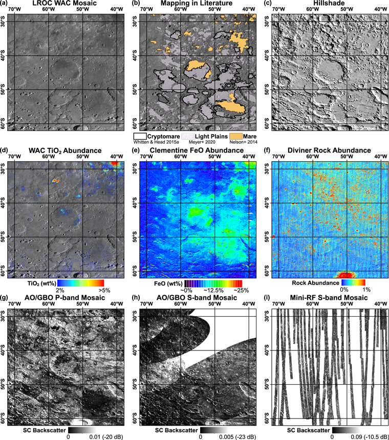
Figure 2. Primary data sets used in this study. (a) LROC WAC global mosaic. (b) Mapped units from the literature (also displayed in Figure 1(b) and included here for ease in comparing data sets) over the WAC mosaic base map. (c) Hillshade created from the LOLA DEM, with simulated shadowing to match ground-based radar images. (d) LROC WAC TiO2 abundances from the 321/415 nm band ratio over the WAC base map (where pixels of no TiO2 data displayed indicate values below the detection threshold of 2%). (e) Derived FeO abundances from the Clementine UVVIS multispectral camera. (f) Rock abundances from the LRO Diviner Radiometer in areal percent. (g) P-band SC backscatter mosaic made from AO/GBO ground-based data. (h) S-band SC backscatter mosaic made from AO/GBO ground-based data. White patches of no data show the areal extent of the gores in this data set. (i) Mini-RF S-band monostatic mosaic, and white patches of no data show the areas of the gores in this data set. The color stretch displayed for each data set remains constant throughout all of the figures in the paper. The maps are shown in a plate carrée cylindrical projection; for scale, the distance between 10° latitude grid lines is ∼300 km, and the distance between 10° longitude grid lines is ∼260 km at a latitude of 30°S and ∼150 km at a latitude of 60°S.
Download figure:
Standard image High-resolution imageWe modeled the thicknesses of the highlands ejecta covering candidate cryptomaria in the region utilizing the radar scattering model from Campbell & Hawke (2005) assuming that the SC radar backscatter varies due to the burial depth of the lava flows (e.g., that the lava flow(s) in the region are all of the same composition and thus that lower radar returns are due to lava flows being closer to the surface and thus occupying more of the subsurface volume sensed by the radar). This calculation (Equation (1) here; Equation (10) in Campbell & Hawke 2005) allows us to estimate the thickness of the highlands-rich ejecta (h) overlying the cryptomare by comparing the raw unitless SC radar backscatter values in areas of possible cryptomaria to the backscatter associated with pure highlands. This calculation assumes that there is a layer of low-loss pure highlands ejecta (of a given dielectric loss tangent, tanδ) overlying either mare basalt or a mixed zone of highland-containing mare.
We perform the calculations using a range of loss tangents from 0.001 (used by Campbell & Hawke 2005 as a rough average lunar loss tangent of pure highlands ejecta) to 0.0002 (lowest-measured lunar loss tangent; Olhoeft & Strangway 1975; Campbell & Hawke 2005). We assume that the lunar regolith has a real component of the dielectric constant (ε') of 2.8 (Campbell & Hawke 2005). The depth to the lossy (i.e., basalt-rich) layer that is calculated is an upper limit, as this equation assumes that there is no significant echo from the surface or losses due to subsurface scattering. Higher rock content in the subsurface lossy layer would cause the calculated depth to decrease. More scattering from the surface or embedded rocks, or a higher loss tangent of the basalts, would lead to shallower burial depths. We used a wavelength (λ) of 70 cm (P-band) and incidence angle (θ) of 30° for the ground-based Arecibo configuration:

3. Results
While areas with known visible maria are associated with areas with low SC radar backscatter, as expected, there are often distinct radar boundaries that do not follow previously proposed mare and cryptomare boundaries from the literature (Figure 3). In some places, the S- and P-band SC backscatter boundaries differ from each other as well.
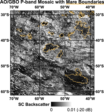
Figure 3. The AO/GBO P-band SC mosaic (Figure 2(d)), with amber boundaries marking the extent of mare locations (Nelson et al. 2014). Note that areas of maria exhibit low SC backscatter, but also that there are additional patches of distinctly low backscatter outside of the areas of known maria. The map is shown in a plate carrée cylindrical projection; for scale, the distance between 10° latitude grid lines is ∼300 km, and the distance between 10° longitude grid lines is ∼260 km at a latitude of 30°S and ∼150 km at a latitude of 60°S.
Download figure:
Standard image High-resolution imageThe mean P-band SC radar backscatter for mare in our mosaic is −27 dB (i.e., a raw unitless value of 0.002, with a standard error of 2.96e-06). While the low SC backscatter areas correspond extremely well to areas mapped by Nelson et al. (2014) to be mare, we find many areas with just as low values of backscatter that extend beyond the boundaries associated with the surface mare (observable in Figure 3; elaborated in the following section). The distribution of low backscatter values suggests that the flow units are more widespread than in previous mapping, and that radar (particularly at P-band) can detect these flows as they extend into the subsurface.
In this section, we first highlight local examples (Section 3.1) where the radar shows clear boundaries of low P-band SC backscatter, including areas where we can visibly track mare units into the subsurface (thus becoming "cryptomaria") based on contiguous regions of low backscatter. Then, we provide results from the regional backscatter density analysis and ejecta thickness calculations (Section 3.2). In the discussion, we propose a stratigraphy with estimates of burial depths across the region.
3.1. Local Examples
3.1.1. Example 1: Extended Cryptomare West of 60°E
In this region (Figure 4), we find a unit of contiguous low backscatter extending toward the northwest and southwest (Figure 4(j), red boundaries with lobes labeled "NW" and "SW", respectively) from a previously mapped mare deposit (Figure 4(b)). The low-backscatter unit occurs in both the P- and S- bands (Figures 4(g)–(i)) and tends to lack elevated TiO2 (Figure 4(d)) or FeO (Figure 4(e)) abundances compared to the nearby mare (except perhaps in the "SW" lobe of the low-backscatter unit, just west of the small mare-infilled crater ∼60°W). This comparison of TiO2 and FeO abundances between areas inside and outside of known maria suggests that there has been little widespread mixing of mafic material (e.g., through regolith gardening) into surface materials here. The Diviner rock abundances tend to be low, particularly in the patch emanating to the northwest (Figure 4(f)), which likely contributes to the lower radar SC backscatter (fewer surface rocks lead to less surface scattering).

Figure 4. Example 1 of a localized area showing the data sets and our interpretation of a cryptomare "flow unit" of low radar backscatter emanating into the subsurface to the northwest ("NW" in Figure 4(j)) and southwest ("SW" in Figure 4(j)) from the surface mare. (a) LROC WAC global mosaic. (b) Units as mapped previously in the literature over the LROC WAC base map; regions of mare from Nelson et al. (2014) are displayed in amber, proposed cryptomare boundaries from Whitten & Head (2015a) are displayed as bold black outlines, and regions of light plains from Meyer et al. (2020) are displayed in white with purple speckles and 50% transparency. (c) Simulated hillshade. (d) LROC WAC-derived TiO2 abundances over WAC base map. (e) Clementine UVVIS-derived FeO abundances. (f). Rock abundances from the LRO Diviner Radiometer. (g) Ground-based AO/GBO P-band SC backscatter mosaic. (h) Ground-based AO/GBO S-band SC backscatter mosaic. (i) Mini-RF S-band monostatic mosaic over the WAC base map. (j) Ground-based P-band SC backscatter mosaic with red markings to draw attention to our new qualitative interpretations based on P-band SC backscatter values. (k) Comparison of the boundaries of mare (amber lines) and cryptomare (black lines) units as mapped previously in the literature (Figure 4(b)) compared to units derived from our regional-scale P-band backscatter analysis in the following section (Section 3.2), with darker blue indicating shallower basalts, and lighter blue (or no blue) indicating deeper basalts.
Download figure:
Standard image High-resolution imageDetection of DHCs and pyroxene led previous investigators (Whitten & Head 2015a) to suggest cryptomare nearby (Figure 4(b)). The contiguous nature of the low-backscatter unit in conjunction with these previous observations suggests that cryptomare is a plausible explanation here. Although the relative contributions of surface rockiness versus subsurface composition on the observed low backscatter are unknown, it is possible that the two factors are related. For example, in the case of a shallowly buried basalt, the thin coating of light plains and/or ejecta material may bury some of the blocky basaltic rocks, leading to lower rock abundances than where the basalts are exposed at the surface. Relatively smooth light plains deposits could provide an alternative explanation for the low rock abundance; however, Meyer et al. (2020) did not map the area associated with the "NW" part of the unit to be light plains (Figure 4(b)), even though it is contiguous with the "SW" part of the unit that is covered in light plains.
The "NW" lobe exhibits low radar backscatter at both P- and S-band as well as low rock abundances, which could also be consistent with a pyroclastic deposit (e.g., Zisk et al. 1977; Gaddis et al. 1985; Campbell et al. 2008). In this area, there are some small fractures, and localized pyroclastic deposits have been proposed nearby to the "NW" lobe. Less than 100 km to the northwest (29.5°S, 64.4°W) are mantled highlands (albeit on a crater floor) that have been identified as a small (174 km2) pyroclastic deposit by Gaddis et al. (2003; at a location called "Lagrange C"). A later survey (Gustafson et al. 2012) searched for previously unidentified pyroclastic deposits using LROC images to characterize local geomorphology (pyroclastic materials appear as diffuse, smooth, mantling deposits that lack effusive lava flow textures) and geologic setting (the presence of nearby rilles, fractures, or other potential source vents provide important contextual evidence for a pyroclastic origin) in concert with Clementine multispectral reflectance data for compositional analyses. Initial screening by Gustafson et al. (2012) of these data near the roughly peanut-shaped maria (which they labeled "Vieta T," with coordinates of 33.4°S, 58.4°W and 33.6°S, 57.2°W) just east of our "NW" low-backscatter lobe caused those authors to consider it as a potential pyroclastic deposit. However, the authors deemed the area inconclusive regarding the presence of pyroclastic deposits and stated that alternative formation mechanisms for irregular or patchy dark deposits include partially obscured mare material or partially exhumed cryptomaria. Therefore, although it is possible that this localized area contains pyroclastic material, in assessing this region as a whole, we suggest that the low-backscatter unit represents a basaltic unit with a variable depth of burial across the scene.
There is a small portion of the area mapped previously to be cryptomare in Whitten & Head (2015a) that is not within our low-backscatter flow unit (just west of the "SW" lobe; Figures 4(b), (g), (j), and (k)). There are two possible explanations for this discrepancy. This portion could be buried deeper than the surrounding cryptomaria (deep enough that it is undetectable by P-band as quantified in Section 3.2), and/or the full boundary of this cryptomaria patch could be different than what was mapped by Whitten & Head (2015a).
3.1.2. Example 2: Multiple Cryptomare Units Extending from a Mare Patch
In this region (Figure 5), we again see areas of low backscatter similar to that of the mare but outside of the previously mapped boundaries of mare and cryptomare. There is an area of higher P-band backscatter (Figure 5(j), yellow arrow) that separates the low backscatter of the large mare patch (which occupies most of the center of the area; Figure 5(b)) and another area of low backscatter ∼30 km to the west (Figure 5(j), red boundary west of yellow arrow). We interpret this separated low-backscatter patch as cryptomare. The close proximity of these units may indicate that the western, low-backscatter patch may be part of the same unit as the mare just east of it, but the intervening area (Figure 5(j), yellow arrow) has been more deeply buried by the heterogenous emplacement of ejecta/light plains material. An alternative explanation for this intervening area of higher backscatter is that there may be a more recent, compositionally distinct flow unit emplaced atop the low-backscatter (higher TiO2/FeO) unit. However, a young mare lava flow has not been previously noted on the surface in this area (Nelson et al. 2014; Figure 5(b)). Additionally, Meyer et al. (2020) mapped this area to be light plains materials, similar to the surrounding areas interpreted as cryptomare (Figure 5(b)). We therefore favor the explanation that this patch is due to heterogeneous ejecta-based embayment rather than embayment by a younger, low-loss basaltic flow.
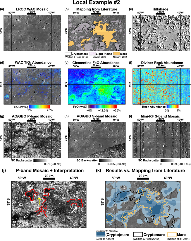
Figure 5. Example 2 of a localized area where maria deposits can be followed into the subsurface by boundaries of contiguous low backscatter in the P-band backscatter image (red and white arrows in Figure 5(j)). The yellow arrow in Figure 5(j) points to a patch of higher SC backscatter, which we interpret as being a location of thicker ejecta burying a basalt unit that exists both east (as exposed mare; Figure 5(b)) and west (as cryptomare) of the patch. (a) LROC WAC global mosaic. (b) Units as mapped previously in the literature over the LROC WAC base map; regions of mare from Nelson et al. (2014) are displayed in amber, proposed cryptomare boundaries from Whitten & Head (2015a) are displayed as bold black outlines, and regions of light plains from Meyer et al. (2020) are displayed in white with purple speckles and 50% transparency. (c) Simulated hillshade. (d) LROC WAC-derived TiO2 abundances over the WAC base map. (e) Clementine UVVIS-derived FeO abundances. (f) Rock abundances from the LRO Diviner Radiometer. (g) Ground-based AO/GBO P-band SC backscatter mosaic. (h) Ground-based AO/GBO S-band SC backscatter mosaic over the WAC base map. (i) Mini-RF S-band monostatic mosaic over the WAC base map. (j) Ground-based P-band SC backscatter mosaic with red markings and colored arrows to draw attention to our new qualitative interpretations based on P-band SC backscatter values. (k) Comparison of the boundaries of mare (amber lines) and cryptomare (black lines) units as mapped previously in the literature (Figure 5(b)) compared to units derived from our regional-scale P-band backscatter analysis in the following section (Section 3.2), with darker blue indicating shallower basalts and lighter blue (or no blue) indicating deeper basalts.
Download figure:
Standard image High-resolution imageIn this same region, a narrow patch of low-backscatter material (Figure 5(j), red boundaries with red arrow) emanates to the southwest from the large mare patch and connects it to a smaller region of mare, which may indicate that these maria are part of the same flow unit with the "neck" between them buried by a very thin coating of ejecta. This "neck" appears as a smooth patch in the LROC WAC data (Figure 5(a)) with increased TiO2 and FeO, similar to the exposed maria on either side (Figures 5(d) and (e)). We also observe that the large mare patch has a contiguous low-backscatter lobe of shallow cryptomare extending ∼30 km further to the east (Figure 5(j), red boundary with white arrow), near latitude ∼35°S. This lobe is also compositionally contiguous with the nearby mare via its moderately elevated (∼12.5%) FeO content (Figure 5(e)). These data support our interpretation that the contiguous unit of low SC radar backscatter is due to the gradual shallow burial of the main central basaltic unit, where the radar allows us to observe the transition from mare to cryptomare.
3.1.3. Example 3: Schickard Crater
Schickard Crater is an interesting case because there are two mare patches at the edges of the crater floor separated by a broad expanse of light-toned materials in between (Figure 6). The boundaries of these two mare patches match well with the boundaries delineating low SC returns in the P-band ground-based data (Figure 6(g)). Despite the clear boundaries of the mare patches in the P-band data, these maria are not apparent in the nominally shallower-sensing S-band data (Figures 6(h) and (i)). The homogenous S-band backscatter may be indicative that the surface within the crater has a large abundance of decimeter-sized boulders that may be causing the S-band signal to scatter, preventing composition (mare versus non-mare) from playing as strong of a role in the S-band backscatter values. This is supported by the Diviner rock abundance map, which shows similar rock abundances across the interior of the crater floor spanning both mare and non-mare areas (Figure 6(f)).

Figure 6. Localized area 3 showing the two mare patches within Schickard Crater. The boundaries of the maria match extremely well to the low P-band SC backscatter, while the S-band SC backscatter and rock abundances are fairly homogeneous across mare and non-mare. We interpret the middle of the crater between the two maria deposits as being particularly deep cryptomare. (a) LROC WAC global mosaic. (b) Units as mapped previously in the literature over the LROC WAC base map; regions of mare from Nelson et al. (2014) are displayed in amber, proposed cryptomare boundaries from Whitten & Head (2015a) are displayed as bold black outlines, and regions of light plains from Meyer et al. (2020) are displayed in white with purple speckles and 50% transparency. (c) Simulated hillshade. (d) LROC WAC-derived TiO2 abundances over the WAC base map. (e) Clementine UVVIS-derived FeO abundances. (f). Rock abundances from the LRO Diviner Radiometer. (g) Ground-based AO/GBO P-band SC backscatter mosaic. (h) Ground-based AO/GBO S-band SC backscatter mosaic over the WAC base map. (i) Mini-RF S-band monostatic mosaic over the WAC base map. (j) Ground-based P-band SC backscatter mosaic with a red boundary indicating an area of deep cryptomare in our new qualitative interpretation based on P-band SC backscatter values. (k) Comparison of the boundaries of mare (amber lines) and cryptomare (black lines) units as mapped previously in the literature (Figure 6(b)) compared to units derived from our regional-scale P-band backscatter analysis in the following section (Section 3.2), with darker blue indicating shallower basalts and lighter blue (or no blue) indicating deeper basalts.
Download figure:
Standard image High-resolution imageThe middle portion of the crater, between the two mare patches, has been proposed to be cryptomare by Whitten & Head (2015a; Figure 6(b)) and others based on the presence of DHCs and a pyroxene signal. However, the P-band backscatter values in this area are not depressed and are similar to surrounding non-mare materials (and not attributable to increased rock abundance). The TiO2 content in the middle of the crater is below detection thresholds (Figure 6(d)), and the FeO content is lower than that in the mare patches (Figure 6(e)). These observations are all consistent with the ejecta cover being thicker in this area, burying the middle portion of basalts relatively deeply (quantified in Section 3.2). Alternatively, it is possible that the middle patch is an area of low titanium and iron content within the lava flow (which is less favored, given Meyer et al. (2020)'s surface observations of light plains here; Figure 6(b)), or that the maria in Schickard Crater were only emplaced locally in these patches on the crater floor after the emplacement of the highlands material, which would indicate that the timing of this system may not be the same as the other areas.
3.1.4. Example 4: An Unusual Radar-dark Region with Sharp Boundaries
In this region (Figure 7), our data suggest that the cryptomare is more extensive than the previously mapped boundaries (Whitten & Head 2015a), following a long strip running northwest–southeast (Figure 7(j), red boundary) across the scene. There is no elevated TiO2 abundance associated with the unit (Figure 7(d)). However, there is a slightly elevated FeO abundance (Figure 7(e)), in addition to lower rock abundances (Figure 7(f)), both of which likely contribute to (or are interconnected to the origin of) the P- and S-band radar data indicating lower relative SC backscatter values here (Figures 7(g)–(i)). While the combination of low radar backscatter and low rock abundance can also be caused by the characteristics of pyroclastic deposits, previous surveys (Gaddis et al. 1985, 20013; Gustafson et al. 2012) have not indicated that this region exhibits any of the geomorphologic, geologic, or spectral characteristics needed to prefer an explosive volcanic origin here.
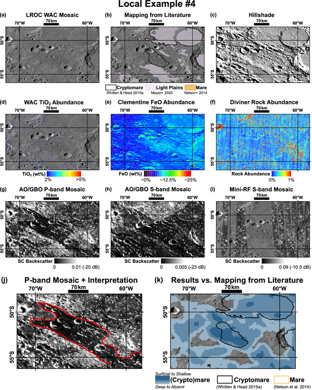
Figure 7. Localized example 4 showing boundaries of low backscatter running northwest–southeast (Figure 7(j)) that encompass a greater extent than the cryptomare in this area as mapped in Whitten & Head (2015a; Figure 7(b)). This cryptomare may have a more FeO-rich (as opposed to TiO2) composition (Figures 7(d) and (e)). The area also exhibits slightly lower rock abundances (Figure 7(f)). (a) LROC WAC global mosaic. (b) Units as mapped previously in the literature over the LROC WAC base map; regions of mare from Nelson et al. (2014) are displayed in amber, proposed cryptomare boundaries from Whitten & Head (2015a) are displayed as bold black outlines, and regions of light plains from Meyer et al. (2020) are displayed in white with purple speckles and 50% transparency. (c) Simulated hillshade. (d) LROC WAC-derived TiO2 abundances over the WAC base map. (e) Clementine UVVIS-derived FeO abundances. (f). Rock abundances from the LRO Diviner Radiometer. (g) Ground-based AO/GBO P-band SC backscatter mosaic. (h) Ground-based AO/GBO S-band SC backscatter mosaic. Note that there is a seam in the S-band mosaic running northeast–southwest across this area causing an artificial boundary in backscatter. However, the pattern of areas of low backscatter relative their surroundings holds true on both sides of the seam. (i) Mini-RF S-band monostatic mosaic over the WAC base map. (j) Ground-based P-band SC backscatter mosaic with red markings to draw attention to our new qualitative interpretations based on P-band SC backscatter values. (k) Comparison of the boundaries of mare (amber lines) and cryptomare (black lines) units as mapped previously in the literature (Figure 7(b)) compared to units derived from our regional-scale P-band backscatter analysis in the following section (Section 3.2), with darker blue indicating shallower basalts and lighter blue (or no blue) indicating deeper basalts.
Download figure:
Standard image High-resolution imageThe hillshade map with simulated shadowing shows that the low radar backscatter in this area is not simply due to a regional surface slope facing away from the radar. Therefore, we rule out topographic effects on the radar signal. We thus attribute this low-backscatter patch to the presence of a shallowly buried cryptomare flow unit (containing more FeO than TiO2) that is more extensive than what was previously mapped (Whitten & Head 2015a).
3.1.5. Example 5: A Complex Area with Likely Changes in Composition and Depth
This is a complicated region (Figure 8) where there are again distinct boundaries in the radar backscatter (Figure 8(j), e.g., red boundary) that are not due to increased surface TiO2 abundances (Figure 8(d)) or topographic shadowing (Figure 8(c)) but may be the result of buried moderate (∼12.5%) FeO content basalts, similar to the overall composition of maria in the region (Figure 8(e)). The observed radar-based boundaries do not match the previously mapped boundaries of maria and cryptomaria. The low-backscatter radar boundaries are consistent and observable in both P- and S-band data (although there is limited coverage of Mini-RF monostatic data), and we interpret this low backscatter as indicative of shallow cryptomaria across the area. Within the area previously mapped in the literature to be cryptomaria, there is a lobe of higher backscatter (Figure 8(j), yellow arrow) that appears to intrude into or superpose the unit of low backscatter, suggesting either multiple compositionally distinct flow units and/or variable burial depth. This example highlights the complicated structure of the region, and some of these complexities in subsurface structure and our ability to distinguish interpretations will be discussed in the following sections.

Figure 8. Local example 5 showing a distinct boundary of low SC backscatter (Figure 8(j), red boundary), with a lobe of higher backscatter (Figure 8(j), yellow arrow) that does not match the boundaries of previously mapped maria or cryptomaria (Figures 8(b) vs. (g)). (a) LROC WAC global mosaic. (b) Units as mapped previously in the literature over the LROC WAC base map; regions of mare from Nelson et al. (2014) are displayed in amber, proposed cryptomare boundaries from Whitten & Head (2015a) are displayed as bold black outlines, and regions of light plains from Meyer et al. (2020) are displayed in white with purple speckles and 50% transparency. (c) Simulated hillshade. (d) LROC WAC-derived TiO2 abundances over the WAC base map. (e) Clementine UVVIS-derived FeO abundances. (f). Rock abundances from the LRO Diviner Radiometer. (g) Ground-based AO/GBO P-band SC backscatter mosaic. (h) Ground-based AO/GBO S-band SC backscatter mosaic. (i) Mini-RF S-band monostatic mosaic over the WAC base map. (j) Ground-based P-band SC backscatter mosaic with red markings and yellow arrow to draw attention to our new qualitative interpretations based on P-band SC backscatter values. (k) Comparison of the boundaries of mare (amber lines) and cryptomare (black lines) units as mapped previously in the literature (Figure 8(b)) compared to units derived from our regional-scale P-band backscatter analysis in the following section (Section 3.2), with darker blue indicating shallower basalts and lighter blue (or no blue) indicating deeper basalts.
Download figure:
Standard image High-resolution image3.2. Regional Backscatter Analysis and Burial Depth Estimates
In order to more quantitatively map the extent of low-backscatter regions, we performed a series of data extractions, show in Figure 9. First, we mapped the pixels (in yellow) where the P-band SC backscatter values are less than the mean of the mare (0.002; Figure 9(a)). Then, we extracted pixels where our approximate hillshade simulation suggested shadowing in the P-band observation (Figure 9(b), red pixels). By subtracting the shadowed pixels from the low-backscatter pixels, we are able to produce our final map of nonshadowed, low-backscatter pixels (Figure 9(c), yellow pixels).

Figure 9. Steps of pixel extraction that went into the regional backscatter analysis. (a) Pixels with P-band SC backscatter <0.002 (mean of the mare in our P-band mosaic) highlighted in yellow over the WAC base map. (b) Pixels in shadow in our simulated hillshade highlighted in red over the WAC base map. (c) Pixels with low backscatter not due to shadowing highlighted in yellow over the WAC base map. The maps are shown in a plate carrée cylindrical projection; for scale, the distance between 10° latitude grid lines is ∼300 km, and the distance between 10° longitude grid lines is ∼260 km at a latitude of 30°S and ∼150 km at a latitude of 60°S.
Download figure:
Standard image High-resolution imageWe performed a point density analysis (Figure 10) on the map of low P-band SC backscatter pixels in nonshadowed regions (Figure 9(c)), and the resulting point densities were partitioned into quartiles. In Figure 10, the dark blue areas contain point densities above the third quartile, the medium blue areas contain point densities between the second (i.e., median) and third quartile, the light blue areas contain point densities between the first and second quartiles, and the areas not colored (i.e., the map displays the background WAC mosaic) are where the point densities are below the first quartile. The means and standard errors of ground-based P-band SC backscatter within each of these four units (excluding pixels in shadow or bright illumination in the hillshade) are provided in Table 1.
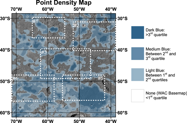
Figure 10. Point density map based on density of pixels with P-band SC backscatter values that are below the mean for the mare (0.002, i.e., −27 dB) and not in hillshade shadow, with color split by quartiles (darker blue indicating a higher concentration of low-backscatter values and lighter blue indicating a lower concentration of low-backscatter values). White dashed boundaries with number labels indicate the five locations highlighted in Section 3.1. The map is shown in a plate carrée cylindrical projection; for scale, the distance between 10° latitude grid lines is ∼300 km, and the distance between 10° longitude grid lines is ∼260 km at a latitude of 30°S and ∼150 km at a latitude of 60°S.
Download figure:
Standard image High-resolution imageTable 1. Mean SC Backscatter Values (Unitless and in dB) and Standard Error of the Mean from Each of the Three Data Sets (AO/GBO P Band, AO/GBO S Band, and Mini-RF S Band) for the Four Quartile Units Resulting from the P-band Regional Backscatter Analysis
| Color Description from Figure 9 | Dark Blue | Medium Blue | Light Blue | Base Map (Transparent) |
|---|---|---|---|---|
| P- band–based point density quartile | >Third quartile | Between second and third quartile | Between first and second quartile | <First quartile |
| Area (km2) | 55,446 | 125,235 | 172,760 | 234,001 |
| Mean P-band SC backscatter ± STE | 0.001 48 ± 1.17e-06 (−28.3 dB) | 0.003 22 ± 9.33 e-06 (−24.9 dB) | 0.004 91 ± 7.38 e-06 (−23.1 dB) | 0.008 42 ± 6.64 e-06 (−20.7 dB) |
| Mean ground-based S-band SC backscatter ± STE | 0.000 961 ± 5.74e-07 (−30.2 dB) | 0.001 61 ± 7.53e-07 (−27.9 dB) | 0.002 19 ± 1.59e-06 (−26.6 dB) | 0.002 89 ± 3.41e-06 (−25.4 dB) |
| Mean Mini-RF S-band SC backscatter ± STE | 0.027 3 ± 4.39e-06 (−15.6 dB) | 0.033 2 ± 6.70e-06 (−14.8 dB) | 0.035 6 ± 7.57e-06 (−14.5 dB) | 0.035 8 ± 7.94e-06 (−14.5 dB) |
Download table as: ASCIITypeset image
We find that the S-band data sets also display the same general backscatter trend as the P-band data set; i.e., the areas of low average P-band backscatter also exhibit low average S-band backscatter (Table 1). However, the two S-band data sets yield different ranges and average values, which has been noted previously (Carter et al. 2017) and is attributed to differences in the basis of polarization of the signals (linear versus circular). Unfortunately, the data coverage gaps in both S-band data sets prevented us from performing the point density analysis done in the P-band data (i.e., Figure 10). The examples in Section 3.1 qualitatively show that the S-band boundaries are often (but not always) similar to the P-band–based boundaries. These results suggest that both P- and S-band data sets are overall most sensitive to the presence of shallow basalts, despite some local areas (e.g., example 3; Figure 6) appearing to be more sensitive to wavelength-scale scatterers and roughness. Average backscatter values, as well as the area (in square kilometers) associated with each point density quartile unit from Figure 10, are provided in Table 1.
In order to estimate the burial depths of these proposed cryptomare units, we first use the average P-band SC backscatter value from the regions in the point density map below the first quartile as representative for the surrounding highlands/light plains material (SCsurroundings) in Equation (1) (Campbell & Hawke 2005). Using the average backscatter values for the three increased point density analysis "units" as SCcryptomare in Equation (1) yields estimates of the maximum depth of burial associated with our point density map (Figure 11). We calculate an "expected" maximum burial depth by assuming that the lunar loss tangent of the highlands ejecta layer atop the basalts is 0.001 (Campbell & Hawke 2005), which yields results of maximum burial depths of 6, 14, and 25 m for the three point density units (above third quartile, second to third quartile, and first to second quartile, respectively). Using an extreme lower limit (lowest ever measured for lunar material) loss tangent of 0.0002 (Campbell & Hawke 2005) provides an upper limit on the maximum burial depth of 28, 70, and 126 m for the units. These two sets of calculations illustrate that there could be a factor of ∼5 or more variation in our estimates of burial depths due to possible compositional variability of the light plains material in the Schiller–Schickard region. We note that these loss tangents are still relatively low compared with most lunar materials. A loss tangent of 0.001 is applicable for materials containing no FeO or TiO2 (Carrier et al. 1991), and 0.0002 is an extreme lower limit and uncommon value. It is unlikely that P-band radar is able to penetrate to >100 m in rocky materials. Additionally, there will also be non-dielectric losses from embedded rocks and fractures that will prevent penetration depths that are that deep. Therefore, we favor the shallower values calculated using a loss tangent of 0.001 but note that the burial depths could be even shallower depending on the composition of the superposing unit (e.g., if typical highlands ejecta contains enough FeO or TiO2 such that the average loss tangent of the ejecta is greater than 0.001) and the structure (fractured and/or blocky) of the light plains material that covers the basalts.
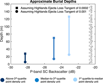
Figure 11. Plot of approximate burial depth calculations vs. the average P-band SC backscatter (in dB) for the three units from the point density analysis assuming two lunar loss tangents (squares and circles). The gray dashed line shows the average SC backscatter value from the regions in the point density map below the first quartile, which we use as representative for the surrounding highlands/light plains material.
Download figure:
Standard image High-resolution image4. Discussion and Interpretations
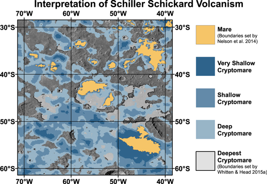
Combining the thickness calculations from Section 3.2 with the map of the point densities of low-backscatter values in Section 3.2 and mapping in the literature of maria and cryptomaria help to detect and infer the subsurface stratigraphic and structural boundaries of cryptomaria visually obscured across Schiller–Schickard (Figure 12). Our results show that most of the Schiller–Schickard region exhibits low P-band SC backscatter emanating from and extending beyond the main areas of mapped maria. In Figure 12, the amber areas (which cover 43,071 km2 within 30–60°S, 40–70°W) constitute maria (as mapped by Nelson et al. 2014). We propose that areas in dark blue (29,150 km2) represent areas where the cryptomare is extremely shallow (<6 m). The areas in medium blue (112,012 km2) are where the cryptomare is buried by up to 14 m of light plains ejecta, and the areas of light blue (169,308 km2) are where the cryptomare is deeply buried (<25 m). The burial depths listed here are based on a loss tangent of the ejecta of 0.001 and will be greater for lower loss tangents (Figure 11). Figure 12 also showcases areas where Whitten & Head (2015a) proposed cryptomaria based on surface geology associated with DHCs and pyroxene spectral signatures, although some parts of these regions do not display a high density of low-backscatter radar signatures. We thus propose that these regions are the areas of deepest cryptomaria (i.e., thickest light plains materials) within the region, covering 39,683 km2. In the areas where the WAC image mosaic base map is displayed with no overlay, we suggest that there is no cryptomare, or that the cryptomare is buried sufficiently deep (at least ∼25 m beneath the surface) as to avoid mixture with the upper decameters through cratering and regolith gardening processes and to evade being sensed by radar data sets. We propose that the total area within the region we mapped (30–60°S, 40–70°W) that contains cryptomare may be up to 350,152 km2, which is 60% of the total area and a factor of 2.7 increase in areal extent as compared to that proposed by Whitten & Head (2015a). Combined with the areas of exposed surface mare, this means that 67% of the region may have been covered in mare basalts.
Figure 12. Interpretation of the region based on the low-backscatter point density map from Figure 10, including mare boundaries from Nelson et al. (2014) in amber and boundaries of the deepest cryptomare (in bold black outlines with gray partially transparent fill) set by mapping from Whitten & Head (2015a) that are not in our "hot spots" of low backscatter. Where the WAC mosaic base map is displayed without overlay, we have no evidence for the presence of cryptomaria. Areas in blue are where we propose that there are cryptomaria based on the P-band radar data (with darker blue indicating that the cryptomaria are shallower and lighter blue indicating deeper). The map is shown in a plate carrée cylindrical projection; for scale, the distance between 10° latitude grid lines is ∼300 km, and the distance between 10° longitude grid lines is ∼260 km at a latitude of 30°S and ∼150 km at a latitude of 60°S.
Download figure:
Standard image High-resolution image
As a test of our hypothesis, we examine the likely source and distribution of the covering of light plains material. Orientale basin is to the northwest of our region of interest; therefore, most of the light plains material superposing the Schiller–Schickard basalts is expected to have been emplaced by the Orientale-forming impact event (e.g., Antonenko et al. 1995; Blewett et al. 1995; Whitten & Head 2015a). It is expected that the ejecta would be thicker (i.e., cryptomaria are buried deeper) approaching the northwest direction and thinner approaching the southeast. Our observations match this interpretation (Figure 12), as the size and number of darker blue (more shallowly buried cryptomaria) increase toward the southeast. In fact, the largest proposed patch of shallow cryptomare is centered near 55°S, 45°W, at the southeastern border of the investigated region. These results are consistent with observations by Whitten & Head (2015a) of an albedo trend across the area, with lower albedos observed toward the southeast, suggesting that the cryptomare is shallower to the southeast (and thus more readily incorporated into the regolith through vertical mixing). Our results of cryptomare locations northwest of Schickard are also consistent with the mapping by Campbell & Hawke (2005) east of Orientale.
Fassett et al. (2011) estimated the average thickness of Orientale ejecta as a function of distance (from the center of Orientale) using a power-law relationship. The northwest corner of the region we investigated here is ∼800 km from Orientale, while the southeast corner is ∼1700 km. The 95% confidence interval of the best-fit parameters of the Fassett et al. power law suggests an ejecta thickness of 430–920 m in the northwest corner of the region and 36–160 m in the southeast corner. These numbers are of the same order of magnitude as the thicknesses we calculate assuming the lower limit on the loss tangent (0.0002; Section 3.2) and about a factor of 10 higher than the thicknesses we calculate assuming an average loss tangent for the ejecta of 0.001. This could suggest that a lower loss tangent (and therefore thicker ejecta) is more applicable in this region. We also note that Equation (1) estimates the thickness of the layer of low-loss pure highlands ejecta overlying the lossy layer, which can be either mare basalt or a mixed zone of highlands containing significant quantities (detectable by the radar) of mare material. Therefore, it may be that the radar data (and thus our estimates of depth) are in many places detecting a subsurface mixed mare/ejecta layer between the ejecta and buried mare flows, rather than the depth to the top of the mare itself. However, in many cases (e.g., examples 1, 2, and 5 in Section 3.1), there are apparent units associated with low radar backscatter that are contiguous with the nearby exposed mare. We therefore favor the interpretation that we are detecting the maria at shallow depths (meters to tens of meters), at least in these areas.
Fassett et al. (2011) emphasized that local variability in ejecta thickness deviating from their power law is common, so our results are not necessarily inconsistent with their estimates. We propose that our results may provide new constraints on the thicknesses and amount of local variability in light plains ejecta across the Schiller–Schickard region. Or, the difference between our reported values of the depth to the lossy layer and the Fassett et al. (2011) estimates of Orientale ejecta thicknesses may offer insight into the thickness of the transition zone of mixed mare/highlands materials that lies between the pure highlands ejecta at the surface and the buried basalts. In either case, the discrepancy in depths suggests that a better understanding of basin impact ejecta is needed in general.
Generally, cryptomaria are considered to be some of the oldest mare lava flows, and as such, these flows have had significantly more time to be covered by ejecta than younger mare flows. In many cases, the radar observations show a continuation of flow units from surface mare to subsurface units. These areas (e.g., examples 1, 2, and 5) suggest that the cryptomaria would likely be the same flow event (and thus the same age) as the exposed mare it is connected to and thus provides estimates on the amount of spatial heterogeneity in ejecta emplacement that resulted in some of the basalt being exposed at the surface (maria) and some being buried (cryptomaria). In this case, all/most of the Schiller–Schickard lava flows formed prior to the events that emplaced the light plains atop the basalts (particularly Orientale). The alternative hypothesis is that the mare and cryptomare flows could represent multiple discrete eruptions from the same vent, with the buried cryptomare flows having been erupted prior to the Orientale-forming event and the surficial mare flows having been erupted separately sometime later.
The floor of Schiller Crater contains light plains material, which was calculated to contain a mixture of ∼40% mare material based on spectral mixing analyses (Blewett et al. 1995). Two origins for the light plains on the floor of Schiller Crater were proposed by Blewett et al. (1995): (1) mare basalt was extruded onto the floor of Schiller, which was then contaminated by the emplacement of highlands materials, or (2) the light plains were deposited as ejecta by the Orientale impact event, and the mare component was from preexisting maria in the surroundings that got incorporated via mixing by secondary cratering and debris surge events. In our analysis, we do not find the floor of Schiller to be a local hot spot of low SC radar backscatter values. Our results thus do not support the presence of widespread buried mare in the floor of Schiller, and we favor the latter origin hypothesis for Schiller's light plains. If there is buried mare in the floor of Schiller, it would be the site of the deepest cryptomare across the region. Our observations combined with the findings of Blewett et al. (1995) also suggest that the P-band radar attenuation is not influenced by light plains with ∼40% exogenic mare (mare incorporated in from the surroundings rather than being buried below). If this is the case, it also supports our interpretation that the low-backscatter regions that we do detect are due to buried basalt flows to which the radar signal is able to penetrate.
Throughout this analysis, we have made the assumption that the proposed cryptomare deposits have static compositions and therefore uniform backscatter properties within a flow unit. This is, however, a simplifying assumption, as even maria exposed at the surface have complex radar backscatter properties associated with multiple flow units of variable compositions and from different eruption episodes (Morgan et al. 2016). Cryptomare also surely contain multiple flows of variable composition but with the additional complexity of being buried by a complicated structure from ejecta emplacement and light plains forming events. Indeed, Whitten & Head (2015b) found significant variation in the pyroxene mineralogies of Schiller–Schickard cryptomare, which they attributed to heterogeneities in the volcanism that occurred. Here we categorize the possible cryptomaria into five "units" by burial depth (Figure 12) for simplicity in understanding the overall subsurface structure of cryptomaria in Schiller–Schickard based on radar observations. However, we emphasize that there are not necessarily just the five distinct units presented in Figure 12, and the actual structure is likely more of a continuum that contains additional finer structure within those five groups. Ultimately, the radar backscatter is a function of multiple processes, and we account for how much the burial depth within each unit may vary if there are flows of different compositions by assuming two different loss tangent values. Given the complexity of the subsurface structure, future radar data collection (including at various viewing geometries in Mini-RF's current bistatic configuration; Patterson et al. 2017) could help to further disentangle the effects of terrain on radar response and characterize lunar volcanism.
5. Conclusions
Radar is an ideal tool for probing the shallow subsurface and allows us to track mare lava flows from the surface into the subsurface and map areas with depressed SC radar backscatter associated with basaltic materials. We find that in the Schiller–Schickard region, there are many distinct radar boundaries that do not follow previously mapped cryptomare boundaries that were based solely on surface geology and spectroscopic signatures. Overall, we conclude that the region contains a large network of buried lava flows, as suggested previously (e.g., Blewett et al. 1995). The buried flows may be 170% more widespread (by area) than recent mapping using surface geochemical analyses (e.g., Whitten & Head 2015a). Our results therefore suggest that cryptomaria volumes based on surface signatures in Schiller–Schickard may have been underestimated, and it is possible that cryptomaria have been underestimated in other areas of the Moon as well. If these results are also applicable to other regions of the Moon, it would suggest that early extrusive volcanism was more prevalent than previously thought, providing important new constraints for models of the Moon's thermal evolution (e.g., Laneuville et al. 2013).
We propose that much of the variability in P- and S-band radar backscatter can be attributed to heterogeneities in the thickness of light plains ejecta atop the region (much of which likely came from the Orientale basin forming event). We find approximate burial depths to a basalt-rich layer ranging from tens of meters in the deepest areas to just a few meters in areas with shallow cryptomaria, which are generally contiguous with known maria. However, burial by ejecta is not the only process that can contribute to variations in radar brightness; lunar lava flows within the maria exhibit multiple flow episodes with variable ilmenite amounts (Morgan et al. 2016). Therefore, it is likely that some of the spatial boundaries we see in the radar data are also different flow units and compositions within the eruptions that formed the cryptomare across Schiller–Schickard.
Our work emphasizes the utility of radar for finding subsurface heterogeneities beyond that which can be detected in the visible and spectral data and provides a new interpretation to the shallow structure of the Schiller–Schickard volcanism. Future work will include examination of other regions with proposed cryptomaria, as well as investigating the cumulative role of viewing geometries and wavelength to pull out the effects of terrain on radar response, aided by new acquisition of bistatic data from the LRO Mini-RF team (Patterson et al. 2017). Additional work to decipher the relative contributions of burial depth versus composition versus surface properties (e.g., rock abundances) to backscatter would aid in the interpretation of cryptomaria, offer improvements to our first-order quantitative estimates of burial depths provided here, and shed light on the evolution of magma composition and dynamics within the lunar interior over time.
The data used in this work are available publicly through the Planetary Data System (PDS) Geosciences Node hosted by Washington University in St. Louis (https://pds-geosciences.wustl.edu/) and the United States Geological Survey's (USGS) Astrogeology Science Center (https://astrogeology.usgs.gov/maps/). High-resolution versions of all figures in this study are available at https://doi.org/10.6084/m9.figshare.20705617. This work was supported by the LRO project, under contract with NASA.