


Abstract
We conducted radar observations of near-Earth asteroid 2019 OK on 2019 July 25 using the Arecibo Observatory S-band (2380 MHz, 12.6 cm) planetary radar system. Based on Arecibo and optical observations the apparent diameter is between 70 and 130 m. Combined with an absolute magnitude of H = 23.3 ± 0.3, the optical albedo of 2019 OK is likely between 0.05 and 0.17. Our measured radar circular polarization ratio of μC = 0.33 ± 0.03 indicates 2019 OK is likely not a V- or E-type asteroid and is most likely a C- or S-type. The measured radar echo bandwidth of 39 ± 2 Hz restricts the apparent rotation period to be approximately between 3 minutes (0.049 hr, D = 70 m) and 5 minutes (0.091 h, D = 130 m). Together, the apparent diameter and rotation period suggest that 2019 OK is likely not a rubble-pile body bound only by gravity. 2019 OK is one of a growing number of fast-rotating near-Earth asteroids that require some internal strength to keep them from breaking apart.
Export citation and abstract BibTeX RIS

Original content from this work may be used under the terms of the Creative Commons Attribution 4.0 licence. Any further distribution of this work must maintain attribution to the author(s) and the title of the work, journal citation and DOI.
1. Introduction
Near-Earth asteroid (NEA) 2019 OK was discovered on 2019 July 24 by Cristovao Jacques, Eduardo Pimentel, and Joao Ribeiro de Barros at Brazil's Southern Observatory for Near Earth Asteroids Research (SONEAR) shortly before its closest approach to Earth. The NEA had an apparent magnitude mV = 14.7 and was close to opposition. 7 The object's orbital information from the JPL Small-Body Database 8 shows the closest approach was on 2019 July 25 01:22 TDB at a distance of 11.2 Earth radii (0.00048 au) from Earth, approaching the planet at a relative velocity of 24.53 km s–1. Its orbital elements include an Earth Minimum Orbit Intersection Distance MOIDE = 0.00029 au. 2019 OK is an Apollo NEA whose highly eccentric orbit (e = 0.76) reaches beyond the orbit of Mars and comes within the orbit of Venus; its sidereal orbital period is 2.55 yr. The 2019 flyby, at a distance of 0.000 48 au, is the closest approach to Earth 2019 OK will have over the time span it can be reliably predicted (1721 to 2116). The next encounter within 0.1 au from Earth will be on 2093 July 28 at a distance of 0.053 au. Prediscovery astrometry was later found from additional observatories, including from Panoramic Survey Telescope and Rapid Response System (Pan-STARRS) in 2017. Discovered near perigee and passing within the orbit of the Moon, 2019 OK should have been categorized as a virtual impactor (e.g., Milani 2004) during this close flyby. Wainscoat et al. (2022) address why the object was not detected earlier, appearing as almost stationary made it undetectable to the surveys as a moving object. Slow-moving nearby objects present the greatest challenge to NEA discovery via surveys. The proximity of 2019 OK to Earth and the potential for future close flybys motivated rapid response from optical and radar facilities to reduce its orbital uncertainties and to physically characterize 2019 OK.
Here, we report the analysis of radar observations and related optical data obtained during the close flyby of 2019 OK soon after its discovery. The use of radar systems for planetary science has been practiced for over 50 years. The two primary radar systems used have been the Arecibo Observatory S-band (2380 MHz, 12.6 cm) planetary radar and the Goldstone Solar System Radar X-band (8560 MHz, 3.5 cm) system. Arecibo's observations, especially during its last decade, have made a critical contribution to the postdiscovery dynamical and physical characterization of newly discovered NEAs. Results from radar observations can include precise measurements of line-of-sight distance and radial velocity of the body and, with sufficient signal and resolution, constraints on scattering properties, size, shape, topographic structure, and spin state. Even nongravitational perturbations due to thermal radiation forces and torques, i.e., the Yarkovsky and YORP effects, can be evaluated as demonstrated by Chesley et al. (2003) and Taylor et al. (2007), respectively. In this paper, first we use the available optical observations for 2019 OK, and we derive a potential diameter limited only by possible geometric albedos. We then present the radar observations and results from continuous-wave and range-Doppler experiments for 2019 OK. From these, we derived some of its physical and dynamical properties (diameter, rotation period, and astrometric corrections). We then explore the cohesion of 2019 OK by presenting the results of the calculation of the Drucker–Prager cohesion criterion, the minimal cohesion needed for 2019 OK to hold itself together. We conclude with a short summary of the results noting the value of rapid-response radar characterization of near-Earth objects.
2. Optical Observations
We use the available optical observations of NEA 2019 OK to evaluate possible diameters based on a range of albedos. 2019 OK was detected simultaneously by different surveys, with the SONEAR's observation being the reported discovery. Optical observations for 2019 OK, including 2017 data from the Cerro Tololo Inter-American Observatory and Pan-STARRS, were reported to the Minor Planet Center 9 and are available in the Near Earth Objects - Dynamic Site (NEODyS-2). 10 Postdiscovery analysis found information from 27 additional observations, including in the Pan-STARRS and the Asteroid Terrestrial Impact Last Alert System (ATLAS-HKO) sky surveys, during its close approach. For this study, we used the apparent magnitude (m) of the target reported by nine observatories between 2017 February 21 and 2019 July 25, those with multiple sequential observations at the smallest phase angle.
The absolute magnitude H, defined as m at zero phase angle and at heliocentric and geocentric distances of 1 au, listed in the JPL Small-Body Database 11 for 2019 OK is H = 23.3 ± 0.3, based not only on the discovery apparition observations in July of 2019, but also on the prediscovery observations since 2017.
The range of solar phase angles reported by NEODyS-2 is quite large, from 6° to 50°; however, this range does not constrain the possible opposition surge (e.g., Belskaya & Shevchenko 2000), if any. Although there were no lightcurves available for 2019 OK, prediscovery data and close-approach observations provide values for m in a variety of filters. Without spectral observations of 2019 OK, there is no preexisting information about its likely taxonomic type. The standard relation between diameter (in km), geometric albedo, and absolute magnitude is given by Equation (1) (i.e., Fowler & Chillemi 1992; Harris & Harris 1997; Pravec & Harris 2007):

We use this relationship to derive the possible diameters for the most common range of optical geometric albedos pV from 0.025 to 0.5 (Pravec & Harris 2007; Thomas et al. 2011) with absolute magnitude H = 23.3 ± 0.3. Figure 1 shows the approximate diameter range of 40 to 200 m for 2019 OK at the aforementioned optical albedo range for the case of H = 23.3 with a solid purple line. We further constrain the size range to 70 to 130 m (denoted by the dotted red line) using the radar images presented in Section 3.2. This size range corresponds to optical albedos of pV from 0.05 to 0.17 for the same H, respectively.

Figure 1. Range of diameters obtained from calculation of Equation (1) for H = 23.3 ± 0.3 as a function of optical albedos pV 0.025 to 0.5. The shaded band is the uncertainty in H. The solid purple horizontal lines denote the limits for a diameter of 40 m and 200 m, respectively, corresponding to mathematically possible diameter limits. The dotted red lines denote the limits of 70 m and 130 m, respectively; corresponding to the most likely diameter range (see Section 3.2).
Download figure:
Standard image High-resolution imageAlbedo and diameter are not independent in this relation, and they carry over some uncertainty especially if the shape is very irregular. This is where radar plays a key role. As we present in the next section, radar data can provide further constraints on the physical and dynamical properties for 2019 OK.
3. Radar Observations
Radar measurements place boundaries on possible rotation periods, diameters, and near-surface bulk density and provide precise astrometric corrections. With the object well located in Doppler frequency, we can further constrain the asteroid's range and apparent diameter from radar delay-Doppler images (Ostro 1993). This object was within the field of view of Arecibo from 2019 July 25 15:30 to 18:17 UTC. Therefore, 2019 OK was observed at Arecibo 17 hr after perigee and 41 hr after its discovery. At the observation time, 2019 OK's nominal distance was 3.8 lunar distances from Earth (0.0097 au) or a light round-trip time (RTT) of ∼10 s with respect to the observing site. The first radar observations were continuous-wave (CW) echo-power spectra (Figure 2). We transmitted a monochromatic, unmodulated circularly polarized wave and received the echoes in both the opposite-sense (as transmitted) circular (OC) and same-sense circular (SC) polarizations as described in Ostro (1993). Zero Doppler frequency marked in Figure 2 refers to the expected location of the object's center of mass in Doppler frequency, which corresponds to a predicted radial velocity that is determined by the predicted ephemeris for a specific observation time and location.

Figure 2. Echo-power distribution over Doppler frequency in terms of standard deviations of the background noise for each scan (1–11; times in UT) of 2019 OK and the weighted sum of all scans (bottom right panel) observed using the Arecibo S-band radar system on 2019 July 25, when the object was at 0.009 11 au and receding from Earth. The center frequency has a consistent offset of about +31 Hz, which corresponds to a line-of-sight velocity correction of 1.95 m s–1. The spikiness is due to self-noise and does not necessarily reflect any physical or compositional characteristics.
Download figure:
Standard image High-resolution imageThe signal is transmitted at the target for as long as the RTT of light to reach and return from the target, minus a 7 s transmit-to-receive switch time; the echo is received for that same amount of time. Due to the close proximity of 2019 OK, the 10 s RTT of the signal (average throughout the observation) only allowed for 3 s of data to be acquired per scan (one transmit–receive cycle). We obtained a total of 49 scans for all modes of observation during half an hour (from 17:45:20 to 18:16:19 UTC). Table 1 lists the summary of observations performed with the S-band radar system at the Arecibo Observatory for 2019 OK on 2019 July 25.
Table 1. Radar Observations of Asteroid 2019 OK
| UT Date | Eph | RTT | Ptx | Baud | Spb | Res | Code | Start-Stop | Runs | |
|---|---|---|---|---|---|---|---|---|---|---|
| yyyy-mm-dd | (s) | (kW) | (μs) | (Hz) | (m) | hhmmss-hhmmss | ||||
| 2019-07-25 | 1 | 10 | 271 | CW a | ... | 0.33 | none | none | 174520-174913 | 11 |
| 2 | 251 | 4.0 | 2 | 15.27 b | 300 | 1023 | 175726-180509 | 21 | ||
| 2 | 286 | 0.5 | 1 | 15.27 b | 75 | 8191 | 181008-181619 | 17 | ||
Notes. UT Date is the universal-time date on which the observation began. Eph is the ephemeris solution number used. RTT is the round-trip light time to the target. Ptx is the transmitter power. Baud is the delay resolution of the pseudo-random code used for imaging; baud does not apply to CW data. Spb is the number of complex samples per baud giving an effective delay resolution of baud/spb. Res is the frequency and range resolution of the processed data. For 2019 OK, we examined several different versions of the images, with different frequency resolutions. Code is the length (in bauds) of the pseudo-random code used. The time span of the received data is listed by the UT start and stop times. Runs (scans) is the number of completed transmit–receive cycles.
a CW data were sampled at a rate of 12.5kHz. b The frequency resolution values for delay-Doppler images (4.0 and 0.5 μs) are determined by the user, they must be less than the code bandwidth.Download table as: ASCIITypeset image
The expected signal-to-noise ratio (S/N) is dependent on four main factors: target distance, target size, target rotation rate, and transmitted power. It is commonly expressed as the ratio of the received power (Prx) to the noise in the received power (Prn). This received power (Prx) is recorded after it is mixed with a reference signal and undergoes transformations, filtering, and amplification (i.e., Ostro 1993). The large collecting area of the 305 m antenna at the Arecibo Observatory allowed us to detect weak echoes, which can be distinguished from noise. We measured the round-trip time delay of the signal echoing off the surface of 2019 OK (related to relative position) and the echo Doppler frequency shift (related to relative velocity) and reported this astrometry for public use to JPL Horizons, 12 where it is combined with optical data to produce a new orbit solution.
3.1. Continuous-wave Spectra
From CW echo-power spectra we can measure various radar properties, such as the radar cross section in each polarization (σOC
, σSC
), the circular polarization ratio (μC
), the bandwidth (B), and the radar albedo ( ), which are related to the physical properties of the target. We obtained 11 transmit–receive cycles (scans) during close to 4 minutes (Table 1). The data reported here were acquired, calibrated, and integrated using standard radar techniques for CW experiments (e.g., Ostro 1993; Black 2002; Magri et al. 2007). All quantitative analysis were performed on unsmoothed spectra. The background noise level is fit and removed to make the mean level zero, and the signal scaled to standard deviations above the background noise. Figure 2 shows a montage of each individual scan and the weighted sum of all 11 scans at 2 Hz effective resolution, Gaussian smoothed to reduce the effects of self-noise. The solid line corresponds to the signal power that is received in the OC sense to that transmitted and the dotted line to the signal power received in the SC sense as that transmitted. The cross sections (σOC
, σSC
) are derived from the integrated echo power in the stated polarization. The OC polarization is dominated by specular scattering with some contribution from diffuse scattering (e.g., Black 2002), while the SC is more representative of the diffuse scattering that takes place due to reflections from rubble, craters, ridges, and other structures on the wavelength scale of the transmitted signal (e.g., Virkki & Muinonen 2016). The average radar cross sections for 2019 OK were σOC
= 620 m2 and σSC
= 205 m2, where each value has a 2% relative uncertainty due to statistical noise and 35% relative uncertainty due to systematic uncertainties in the calibration. This estimated 35% systematic uncertainty is larger than the standard 25% at Arecibo because the pointing was poorer than normal due to cable elongation in hot weather.
), which are related to the physical properties of the target. We obtained 11 transmit–receive cycles (scans) during close to 4 minutes (Table 1). The data reported here were acquired, calibrated, and integrated using standard radar techniques for CW experiments (e.g., Ostro 1993; Black 2002; Magri et al. 2007). All quantitative analysis were performed on unsmoothed spectra. The background noise level is fit and removed to make the mean level zero, and the signal scaled to standard deviations above the background noise. Figure 2 shows a montage of each individual scan and the weighted sum of all 11 scans at 2 Hz effective resolution, Gaussian smoothed to reduce the effects of self-noise. The solid line corresponds to the signal power that is received in the OC sense to that transmitted and the dotted line to the signal power received in the SC sense as that transmitted. The cross sections (σOC
, σSC
) are derived from the integrated echo power in the stated polarization. The OC polarization is dominated by specular scattering with some contribution from diffuse scattering (e.g., Black 2002), while the SC is more representative of the diffuse scattering that takes place due to reflections from rubble, craters, ridges, and other structures on the wavelength scale of the transmitted signal (e.g., Virkki & Muinonen 2016). The average radar cross sections for 2019 OK were σOC
= 620 m2 and σSC
= 205 m2, where each value has a 2% relative uncertainty due to statistical noise and 35% relative uncertainty due to systematic uncertainties in the calibration. This estimated 35% systematic uncertainty is larger than the standard 25% at Arecibo because the pointing was poorer than normal due to cable elongation in hot weather.
The ratio of the radar cross sections (σSC /σOC ) is the circular polarization ratio (μC ). It serves as an initial estimate of surface roughness (Ostro 1993; Black 2002; Virkki & Muinonen 2016) and has been linked to composition by correlation to some taxonomic types (Benner et al. 2008; Aponte-Hernández et al. 2020). We measured a circular polarization ratio of 0.33 ± 0.03 for the weighted sum of all scans. This indicates that 2019 OK is unlikely to be a V-type (μC ≈ 0.603 ± 0.088) or an E-type (μC ≈ 0.892 ± 0.079) asteroid, and is more likely to be an S-type (μC ≈ 0.26 ± 0.05) or a C-type (μC ≈ 0.285 ± 0.12) body; the latter one is favored (Benner et al. 2008; Thomas et al. 2011).
The measured Doppler bandwidth (B) depends upon the object's rotation period, diameter, and the subradar latitude. We used Equation (2) (Ostro et al. 2002), in which the rotation period (Prot
) is expressed in terms of the diameter (D), wavelength (λ), and subradar latitude (δ). We assume an equatorial view (δ = 0,  ), to obtain a range of possible rotation rates at the measured bandwidth:

To determine the bandwidth, we analyzed the data in each individual unsmoothed CW scan, and then summed over all scans to obtain an echo's edge-to-edge bandwidth of 38 ± 2 Hz. This bandwidth is significantly larger than what is typically seen in small NEAs (D < 200 m) of ∼1–10 Hz, which is an indicator of a rapid rotation rate. Bandwidths observed in individual scans reached a minimum of 31 Hz and a maximum of 43 Hz, but there is no clearly repeated pattern, in part due to short observation time and intervals of observations being on the same order as the rotation period. We performed a weighted average of the edge-to-edge bandwidth measurement of each scan's echo, yielding a bandwidth of 39 ± 2 Hz. Each scan measures the instantaneous bandwidth, and variation over time is expected for a rotating nonspherical object. For the above bandwidths and a diameter of no less than 70 m and no more than 130 m (see Section 3.2), we find the rotation period (Prot
) can range from approximately 0.05 hr to 0.09 hr (3 to 5 minutes), respectively, not excluding a faster rotation period for nonequatorial subradar latitudes ( ).
).
Another key product from radar observations is the derivation of the radar albedo ( ), which is a measure of surface reflectivity where an albedo of one denotes a perfect reflector (assuming a spherical target; Ostro 1993; Magri et al. 2001; Black 2002). To first order, the radar albedo can be calculated as
  , where the projected area (AProj
) is based on the presumed diameter and assuming a spheroidal shape. We obtain
, where the projected area (AProj
) is based on the presumed diameter and assuming a spheroidal shape. We obtain  to be in the range of 0.16 (D = 70 m) to 0.047 (D = 130 m). Using the model developed by Hickson et al. (2018, 2020), we estimated the near-surface mass density of 2019 OK. In their work, they presented an expansion of Magri et al. (2001) to calculate near-surface bulk densities (ρbulk
) for NEAs using radar albedos and compositional information from meteorite analogs.
to be in the range of 0.16 (D = 70 m) to 0.047 (D = 130 m). Using the model developed by Hickson et al. (2018, 2020), we estimated the near-surface mass density of 2019 OK. In their work, they presented an expansion of Magri et al. (2001) to calculate near-surface bulk densities (ρbulk
) for NEAs using radar albedos and compositional information from meteorite analogs.
From the relationship between  and the Fresnel reflection coefficient (R) (
 ), where g is the backscatter gain (assumed to be 1.2), the near-surface permittivity
  can be estimated by the relationship between the circular polarization ratio (making certain assumptions when estimating, R) and near-surface density. We find an approximate permittivity of 4.65 (D = 70 m) and 2.22 (D = 130 m). It is important to note that these surfaces are not homogeneous and subsurface scattering from voids, grain composition variation, and diffuse scattering play a role (Hickson et al. 2018) in our estimated values for . The used model does not necessarily account for individual cases, which could also play a role.
We then take the same assumptions regarding backscatter gain (g) and diffuse circular polarization as in Equations (5) and (7) of Hickson et al. (2020) to calculate the near-surface bulk density of 2019 OK. We include our own values for σOC and μC (Table 2) and assume 2019 OK is C- or S-type, where the grain density of the meteorite analog is roughly 2.8 to 3.5 g cm−3 (Consolmagno et al. 2008). We obtained ρbulk = 1.2 g cm3 for D = 70 m with a porosity of 0.6, and ρbulk = 0.8 g cm−3 for a 130 m object with a porosity of 0.8. By inspection, of these calculation one can see that some level of cohesion is necessary to hold the asteroid together against the disintegration due to centrifugal forces. We explore this further in Section 4.
Table 2. Radar-derived Physical Parameters for 2019 OK
| Parameter | Value |
|---|---|
| Absolute Magnitude (H, mag) | 23.3 ± 0.3 |
| Diameter (D, m) | 70 to 130 |
| Rotation Period (Prot , hr) | 0.05 to 0.09 |
| Geometric Albedo (pV) | 0.05 to 0.17 |
Radar albedo (
| 0.05 to 0.16 |
| Triaxial ratios-Elongation (a: b) | 1.16:1 |
| Circular polarization ratio (μC ) | 0.33 ± 0.03 |
| Bandwidth (B, Hz) | 39 ± 2 |
| OC cross section (σOC , m2) | 620% ± 35% |
| SC cross section (σSC , m2) | 205% ± 35% |
| Minimum cohesion (k, Pa) | 350 |
Download table as: ASCIITypeset image
3.2. Delay-Doppler Imaging
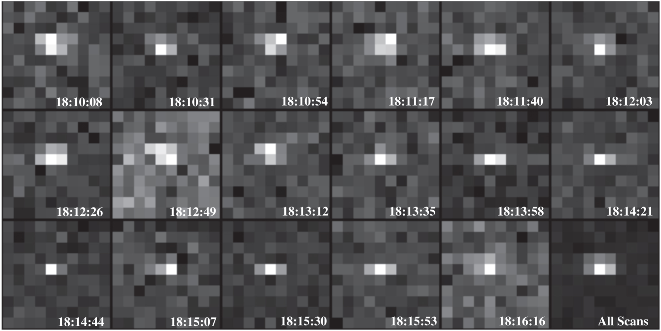
When the target's S/N is high enough, we can resolve the echo in delay (range) and Doppler frequency by transmitting a coded waveform with a characteristic modulation interval known as the baud (e.g., Taylor et al. 2019). For this observation, phase modulation bandwidths used were 0.25 MHz for a 4 μs baud and 2 MHz for a 0.5 μs baud. The 17 scans shown in Figure 3 correspond to the 0.5 μs phase modulation, with a range resolution of 75 m per pixel in delay. From Figure 3, we see that all signals were contained within one or two range bins for 0.5 μs images, rendering it essentially unresolved at a 75 m resolution. The images from 18:10 to 18:13 span two pixels, and those from 18:13 to 18:15 are in a single row (75 m in range). The last image at 18:16 appears to be in two rows again, with the pixel in the second row at 4.7σ.

Figure 3. Range–Doppler images of each scan (1–17, left to right and top to bottom) and the sum of all 17 scans (bottom right frame) using 0.5 μs baud with a resolution of 75 m per pixel in range and 15.3 Hz in Doppler. Delay (range) increases along the vertical axis from bottom to top, and Doppler increases along the horizontal axis from left to right in each frame. The signals are spread over two to three columns (Doppler frequency) and one or two rows (delay) throughout the sequence. Total observation time 6.18 minutes with 3 s per scan.
Download figure:
Standard image High-resolution imageWe calculated the image drift (a slow but steady variation in the target's observed delay, due to slight errors in the ephemeris; see Section 3.3) by comparing the ephemeris used for the observation with the ephemeris from weeks later which incorporated all of the available astrometry, both from the radar observations and available optical observations. If some of the change in the signal position was due to range drift, it would be in the downward direction. Drift cannot explain the last image compared to previous ones. There must be a dimension of the asteroid that is at least 70 m to consistently span two pixels in about half the images. These radar estimates do not necessarily exclude smaller dimensions in some orientations, such as those discussed in Section 2 (D < 70 m). The object could have a larger diameter and be somewhat elongated, giving a similar variation in the 0.5 μs images. In all, the object could be big enough to fill multiple pixels, or be small but split between two pixels; hence, we adopt 70–130 m as the most likely size range for 2019 OK.
In an attempt to extract as much information as possible from the data, we extracted the bandwidths from the delay (range)–Doppler scans (Figure 4). The bandwidth variation did not present any obvious periodicity. The average bandwidth for the 21 scans (63 s of data) of the 4 μs set was 40 Hz (3.8 Hz resolution). For the 0.5 μs data, the average was of 39 Hz (3.8 Hz resolution) in a set of 17 scans (51 s of data). The limited observation duration and unresolved size for 2019 OK did not allow us to obtain shape information. However, the small change in bandwidth and changes in range extent suggest a nonspherical body.

Figure 4. Exploration of bandwidth variation for the data using waterfall plots (spectrograms) for the specific mode of observation. Top box shows the CW observations. The raw data from each scan have been smoothed with an 11-point boxcar (rectangular) filter, giving an effective frequency resolution of 3.7 Hz. This is about the same as the 3.8 Hz frequency resolution of the 4 μs and 0.5 μs images. Middle and bottom boxes (range–Doppler) and delay-Doppler observations for the region with 2019 OK's signal from the 4 and 0.5 μs observations. These data have been processed to have a frequency resolution of 3.8 Hz.
Download figure:
Standard image High-resolution image3.3. Astrometry
Immediately after the CW observations, we used the JPL On-Site Orbit Determination software (OSOD; Ostro 1996) to update the observing ephemeris in real time and improve the 3σ uncertainties on pointing, Doppler, and range. The center of the echo in the CW data was displaced by +31 Hz relative to the optical-only prediction (a ∼0.5σ correction relative to the 190 Hz 3σ uncertainty of Ephemeris 1), which translates to a correction in the line-of-sight velocity of 1.95 m s−1 for the Doppler-only correction to Ephemeris 1. Refitting the orbit using the Doppler correction produced Ephemeris 2, which predicted the RTT to 2019 OK to be reduced by 721.8 μs or, equivalently, that 2019 OK was 108 km closer to Earth. As discussed in Section 3, an important capability of radar techniques is the ability to measure the Doppler frequency shift and range with high precision. For the ranging and imaging, the submitted delay astrometry corresponds to line-of-sight distance corrections of −21.81 μs (−3.27 km) for 4 μs data and −22.59 μs (−3.39 km) for 0.5 μs data (Figure 3), showing a range drift of almost the same amount, while changing observation setup (5 minutes). These radar measurements reduced the uncertainties in 2019 OK's position at the time of our observations (18:00 UTC on 2019 July 25) by a factor of 4 in plane-of-sky position, a factor of 20 in Doppler frequency, and a factor of 1500 in range.
The orbit condition code or uncertainty parameter is given in relation to the in-orbit longitude runoff in seconds of arc per decade, and it quantifies the uncertainty of an orbital solution considering the uncertainties in the perihelion passage time and in the orbital period. It is an integer ranging from 0 (runoff <1.0 arcsec per decade) to 9 (runoff > 146,502 arcsec per decade) 13 ; it is derived from the Q criterion in Marsden et al. (1978). Based on 31 optical measurements, 2019 OK's U parameter was 6. After adding one Doppler and two delay measurements to the orbit solution computation (Arecibo solution #3), the Earth-encounter predictability window was increased, from the discovery apparition (2019) only, to over 100 years, revealing the closest currently predicted Earth encounter to be in 174 years, at a distance of 0.027 46 au on 2196 February 24. The uncertainty parameter was reduced to U = 4.
4. 2019 OK Cohesion
4.1. Theory and Methods
The first certain detection of a fast-rotating asteroid (FRA), one that is rotating significantly faster than 2.1 hr, was 1998 KY26 with a rotation period of Prot = 0.18 hr (10.8 minutes), H = 25.6, and a diameter of 30 m (Ostro et al. 1998; Warner et al. 2009). From the Light Curve Database (LCDB) 2020 May release (Warner et al. 2009), we find 165 asteroids with rotation periods equal to or shorter than the slowest rotation period of 2019 OK, Prot < = 0.14 hr, assuming a D = 200 m (see Section 2). Figure 5 shows where 2019 OK is located with respect to the small fast rotators and the general asteroid population.

Figure 5. Highlight of the location of 2019 OK, in terms of H magnitude versus rotation period (Prot ), among the general asteroid population (including Main Belt Asteroids (MBA) and NEAs) from the Light Curve Database (Warner et al. 2009) 2020 May release with quality factors greater than or equal to 2.
Download figure:
Standard image High-resolution image
Two regimes govern the spin limits for general solids: the strength regime (D < 300 m) and the gravity regime (D > 10 km) (Pravec & Harris 2000). The limits to the macroscale composition of the case of fast-rotating bodies have been shown by several authors (e.g., Pravec & Harris 2000; Holsapple 2007; Polishook et al. 2016, 2017 and references therein) to be governed by the internal strength of the body. Monoliths (with a rugged surface) or rubble piles with enough cohesion rendering them capable of holding their structure via Van der Waals forces (i.e., Scheeres et al. 2010) are examples of objects requiring some internal strength to keep them from flying apart. Following the aforementioned works (Pravec & Harris 2000; Holsapple 2007; Polishook et al. 2016, 2017), we calculated the Drucker–Prager (D-P) yield criterion. The D-P criterion is presented here as in Polishook et al. (2016), as a dependency on two constants, the cohesion k and a slope constant Φ, which, in turn, depends only on the angle of friction ϕ ( ), which we set at ϕ = 35°. With this angle, we can constrain the body's minimum cohesion. The cohesion increases only slightly with increasing friction angle. More details are provided in Holsapple (2007) and Polishook et al. (2017). To obtain k from Equation (8) in Polishook et al. (2016), we first solved their Equations (2) to (4), which define the shear stresses average in vector form. For this work, the density is denoted by ρ given in g cm−3, Prot
is the object's rotation period converted to angular frequency, Gc
is the gravitational constant (6.673 × 10⁻¹¹ m3 kg−1 s−2), and Axyz
are dimensionless quantities that depend only on the asteroid triaxial ratios as in Polishook et al. (2016). Here we used Ax
= Ay
= Az
= 2/3 values as Holsapple (2007), where a, b, and c denote the axis radius. In the next section, we use the methods above to calculate the cohesion for 2019 OK. We used the published work for cohesion for 2001 OE84 (Polishook et al. 2017) and 2005 GD65 (Polishook et al. 2016) as validation of our methods and results.
), which we set at ϕ = 35°. With this angle, we can constrain the body's minimum cohesion. The cohesion increases only slightly with increasing friction angle. More details are provided in Holsapple (2007) and Polishook et al. (2017). To obtain k from Equation (8) in Polishook et al. (2016), we first solved their Equations (2) to (4), which define the shear stresses average in vector form. For this work, the density is denoted by ρ given in g cm−3, Prot
is the object's rotation period converted to angular frequency, Gc
is the gravitational constant (6.673 × 10⁻¹¹ m3 kg−1 s−2), and Axyz
are dimensionless quantities that depend only on the asteroid triaxial ratios as in Polishook et al. (2016). Here we used Ax
= Ay
= Az
= 2/3 values as Holsapple (2007), where a, b, and c denote the axis radius. In the next section, we use the methods above to calculate the cohesion for 2019 OK. We used the published work for cohesion for 2001 OE84 (Polishook et al. 2017) and 2005 GD65 (Polishook et al. 2016) as validation of our methods and results.
4.2. Cohesion for 2019 OK
We begin by estimating the axial ratio of 2019 OK by approximating the lightcurve amplitude. We chose the ATLAS (T05) data set listed on NEODyS-2
14
for this estimate because it provided a uniform sample (eight observations) over a long enough interval to cover multiple rotations (0.63 hr), at a low phase angle (≈10°). The apparent change in magnitude was  mag. The corresponding flux ratio (e.g., Gaffey 1989) is 1.36. The flux is proportional to the apparent area of the body at the time of observation (Equation (3)). Then, the maximum change in magnitude as the object rotates (the lightcurve amplitude) is an estimate of the change in that area. We take the square root of the area ratio to obtain the axial ratio, a/b = 1.16. This is dependent on the viewing geometry, but is at least a lower bound:

To estimate limits of cohesion (k) for 2019 OK, we studied two shapes: a sphere and an ellipsoid. We considered densities of 1 to 3 g cm−3 for the ranges of rotation rates and diameters mentioned earlier (Sections 2 and 3). For an ellipsoid, the axial ratios define constants depending only on the shape to derive k for a given object (Polishook et al. 2016). Using Equation (3) (for the case of the ellipsoid), we assumed a prolate shape with axial ratios of 1.16:1:1. The apparent diameter boundary range of D = [70: 130 m], in average, needs a minimum cohesion to avoid catastrophic disruption is between 350 Pa and 400 Pa for the case of the sphere at a density of 1 g cm−3 as well as for the ellipsoid at same density at the smallest diameter (70 m). For larger sizes or higher densities, the necessary cohesion increases up to 1 kPa for the largest diameter (130 m) at highest density (3 g cm−3). In comparison, Earth mineral aggregates are 1–100 kPa for fractured rocks and up to a few MPa for crystalline rocks (i.e., Turcotte & Schubert 1982). However, this strength is much less than even the weakest rocks seen on Earth, and is much weaker than any meteorite that has survived travel through the Earth's atmosphere.
5. Summary
Rapid-response planetary radar systems are a fundamental asset for postdiscovery physical and orbital characterization of near-Earth objects. With only 16 hr from perigee passage and 41 hr from the discovery to radar characterization at the Arecibo Observatory, these observations of 2019 OK demonstrate the value of rapid-response systems. The object was quickly receding from the Earth, which reduced the detectability with the radar system (40 times weaker S/N in the next day), presenting this as the one and only opportunity to provide radar-derived astrometry and physical characterization. Physical characteristics of 2019 OK derived from radar observations are summarized in Table 2.
The circular polarization ratio (μc ) of 0.33 indicates 2019 OK is likely a C-type rather than a S-type if we take the relatively low geometric albedo into consideration (e.g., Thomas et al. 2011). The radar images suggest a diameter of 70 to 130 m. At the time of the observations, the radar astrometry reduced Doppler and delay uncertainties up to 99.93% compared to the initial optical-only ephemeris. Refitting the orbit after submitting the first astrometry correction (Doppler), the new cumulative prediction of distance was improved by 112 km. Subsequent astrometry reporting from range–Doppler data gave corrections on the order of 3 km, highlighting the precision of this technique. Depending on the orbital trajectory and object size, these measurements can take objects off the virtual impactor lists, such as in the recent case of 2020 NK1 (Venditti et al. 2020). In the case of 2019 OK, our radar observations secured the orbit for the next 100 years.
The minimum cohesion needed for the asteroid to not deform due to its rotation rate is at least 350 Pa. This value is much less than the internal strength of fractured Earth rocks. These are minimum required cohesion values and the actual strength could be much higher. In all, these radar observations enabled constraints on geometric albedo, rotation, diameter, a more precise understanding of the asteroid's position and velocity, and with that a more accurate projection of its future trajectory, highlighting the importance of powerful radar systems like that of Arecibo Observatory.
This research was funded by NASA through the Near-Earth Object Observations program under grant No. 80NSSC19K0523. The Arecibo Observatory is a facility of the National Science Foundation operated under cooperative agreement by the University of Central Florida in alliance with Yang Enterprises, Inc. and Ana G. Mendez University System. Part of this work was performed at the Jet Propulsion Laboratory, California Institute of Technology, under contract with NASA. This work made use of the NASA/JPL Horizons On-Line Ephemeris System and NASA's Astrophysics Data System Bibliographic Services. The authors would like to thank the Arecibo Observatory staff, especially Mr. Victor Negron and Mr. Juan Marrero, as well as the Arecibo Observatory Management Team. The authors thank the anonymous reviewers who helped improve this manuscript.
Facility: The Arecibo Observatory - .
Software: OSOD (Ostro 1993), Radar Decode.
Footnotes
- 7
- 8
- 9
- 10
- 11
- 12
- 13
- 14