


Abstract
The TRAPPIST-1 Habitable Atmosphere Intercomparison (THAI) project was initiated to compare 3D climate models that are commonly used for predicting theoretical climates of habitable zone extrasolar planets. One of the core models studied as part of THAI is ExoCAM, an independently curated exoplanet branch of the National Center for Atmospheric Research Community Earth System Model (CESM), version 1.2.1. ExoCAM has been used for studying atmospheres of terrestrial extrasolar planets around a variety of stars. To accompany the THAI project and provide a primary reference, here we describe ExoCAM and what makes it unique from standard configurations of CESM. Furthermore, we also conduct a series of intramodel sensitivity tests of relevant moist physical tuning parameters while using the THAI protocol as our starting point. A common criticism of 3D climate models used for exoplanet modeling is that cloud and convection routines often contain free parameters that are tuned to the modern Earth, and thus may be a source of uncertainty in evaluating exoplanet climates. Here, we explore sensitivities to numerous configuration and parameter selections, including a recently updated radiation scheme, a different cloud and convection physics package, different cloud and precipitation tuning parameters, and a different sea ice albedo. Improvements to our radiation scheme and the modification of cloud particle sizes have the largest effects on global mean temperatures, with variations up to ∼10 K, highlighting the requirement for accurate radiative transfer and the importance of cloud microphysics for simulating exoplanetary climates. However, for the vast majority of sensitivity tests, climate differences are small. For all cases studied, intramodel differences do not bias general conclusions regarding climate states and habitability.
Export citation and abstract BibTeX RIS

Original content from this work may be used under the terms of the Creative Commons Attribution 4.0 licence. Any further distribution of this work must maintain attribution to the author(s) and the title of the work, journal citation and DOI.
1. Introduction
Over the past decade, 3D climate models have been commonly used to study the climate, habitability, and potential observable phenomena of terrestrial extrasolar planets. There are numerous 3D climate models that are currently deployed for this purpose, including the Laboratorie de Météorologie Dynamique Generic (LMD-G) climate model (Wordsworth et al. 2011; Leconte et al. 2013a, 2013b, 2015; Bolmont et al. 2016; Turbet et al. 2016, 2018; Fauchez et al. 2019; Charnay et al. 2021; Lefèvre et al. 2021), the NASA Goddard Institute for Space Studies Resolving Orbital and Climate Keys of Earth and Extraterrestrial Environments with Dynamics (ROCKE-3D) climate model (Way et al. 2016, 2017; Fujii et al. 2017; Way et al. 2018; Aleinov et al. 2019; Colose et al. 2019, 2021; Del Genio et al. 2019; Jansen et al. 2019; Guzewich et al. 2021; Kane et al. 2021), the UK Met Office Unified Model (UM; Boutle et al. 2017; Mayne et al. 2019; Boutle et al. 2020; Sergeev et al. 2020), the National Center for Atmospheric Research (NCAR) Community Earth System Model (CESM; Shields et al. 2013; Yang et al. 2013, 2014, 2019b; Hu & Yang 2014; Kopparapu et al. 2016; Shields & Carns 2018) a growing list of other codes (Abe et al. 2011; Rauscher & Menou 2012; Haqq-Misra & Kopparapu 2014; Popp et al. 2016; Hammond & Pierrehumbert 2018; Ding & Wordsworth 2020; May & Rauscher 2020; Paradise et al. 2021), and ExoCAM, which is a branch of CESM designed specifically for exoplanets, whose description is the focus of this paper. Terrestrial exoplanet climate models typically branch from Earth climate system models that were created and continue to be supported by national modeling centers. While these exoplanet branches can leverage the utilities of their parent Earth model, they often diverge from their parent models in meaningful ways. Such is the relationship between ExoCAM and its parent model, CESM. Thus, it is important to provide definitive descriptions for exoplanet and planetary code branches for community reference (e.g., Way et al. 2017). The purpose of this paper is twofold. First, we provide a description and primary reference for the ExoCAM model, which includes the first presentation of a recent major overhaul to the radiative transfer scheme. Second, we conduct a series of intramodel climate sensitivity tests with ExoCAM. Starting from the TRAPPIST-1 Habitable Atmosphere Intercomparison (THAI) protocol (Fauchez et al. 2020), we test the model's sensitivity to a number of key tunable parameters and settings related to clouds, convection, precipitation, and sea ice to illustrate the robustness of the model's results for simulating habitable terrestrial extrasolar planets.
ExoCAM is an independently supported branch of NCAR CESM version 1.2.1, which facilitates simulations of generic planetary atmospheres. ExoCAM operates as a patch for CESM. The user must first download the core CESM code, which is freely available and provided by NCAR, 7 before modifying CESM with ExoCAM-specific configuration scripts and source code, also freely available and provided by the lead author on GitHub. 8 Importantly, note that ExoCAM is accompanied by a radiative transfer code for 3D climate models developed by the lead author, ExoRT, 9 which must also be downloaded by the user and linked with ExoCAM and CESM. ExoCAM and ExoRT are designed to be used together, with the ExoCAM GitHub repository containing system files, source code files, initial condition files, namelists, and the documentation needed to install and run 3D climate simulations in tandem with CESM, and the ExoRT GitHub repository containing all files needed for flexible radiative transfer calculations. Several years ago, ExoRT was separated from ExoCAM into its own repository in order to facilitate standalone 1D radiative transfer calculations, which significantly eases model development and validation demands for the radiative transfer component. In this paper, any reference to ExoCAM implicitly includes the linked capability of ExoRT.
ExoCAM and ExoRT were first made available to the public on Github in 2018 November. At the time of finalizing this paper, there have been a total of 37 papers published or accessible on arXiv by 20 different lead authors that use ExoCAM, whether in its entirety, by leveraging specifically credited component modules, or by leveraging specifically credited model outputs for extensive analysis as a central part of the work. ExoCAM has been well-received and well-used since being made public. ExoCAM, and its ancestral versions, have been employed for a wide variety of studies, including the Faint Young Sun Paradox for Earth (Wolf & Toon 2013, 2014a), high-CO2 atmospheres (Wolf et al. 2018; Zhang et al. 2021), runaway and moist greenhouse thresholds for Earth (Wolf & Toon 2014b, 2015), Earth-like extrasolar planets (Wolf et al. 2017; Adams et al. 2019; Kang 2019a, 2019b, 2019c), habitable zone exoplanets around M-dwarf stars (Kopparapu et al. 2017; Wolf 2017; Haqq-Misra et al. 2018; Komacek & Abbot 2019; Komacek et al. 2019, 2020a, 2020b; Wolf et al. 2019; Yang et al. 2019a; Hu et al. 2020; Rushby et al. 2020; Suissa et al. 2020b; Wei et al. 2020; Zhang & Yang 2020; Chen et al. 2021; May et al. 2021; Song & Yang 2021), planets in circumbinary systems (Wolf et al. 2020), and model intercomparison studies (Yang et al. 2016, 2019b; Fauchez et al. 2020, 2021; Sergeev et al. 2021; Turbet et al. 2021). ExoCAM results have also been used off-line in projects to drive photochemistry and observability studies (Afrin Badhan et al. 2019; Suissa et al. 2020a).
ExoCAM is one of the four core 3D climate models used in the THAI project (Fauchez et al. 2020), alongside LMD-G, ROCKE-3D, and UM. The THAI project arose from conversations at the NASA Habitable Worlds Conference in Laramie, WY in 2017 November. It was determined that an important step forward for the growing exoclimate modeling community was to engage in a formal model intercomparison process. This paper describing ExoCAM is part of a collection of papers that have emerged from the THAI project and are featured in this special edition of the Planetary Science Journal (Fauchez et al. 2021; Sergeev et al. 2021; Turbet et al. 2021). The THAI project also led to a community workshop, the proceedings of which are discussed in the THAI workshop report (Fauchez et al. 2021). The THAI project aims to compare and cross-validate 3D climate models that are commonly used for predicting theoretical climate states of habitable zone extrasolar planets while using TRAPPIST-1e as the target object. We refer readers to the other papers in the series for detailed results on the climate states and theoretical observables among the four primary models. This paper provides an addition to the THAI series of papers, for the reader interested in taking a deeper dive into ExoCAM and its intramodel sensitivities.
2. ExoCAM Description
As introduced in Section 1, ExoCAM is a modeling package designed to be used in tandem with NCAR CESM version 1.2.1 to facilitate flexible modeling of extrasolar planetary atmospheres. In recent years, interest in 3D exoplanet atmosphere modeling has exploded, but the road to proficiency for new users entering into the field is often steep and arduous. Furthermore, the real time and computing time required for full-cycle science (project genesis, model development, simulations, analysis, and publication) with 3D climate models means that current 3D exoclimate modeling groups are often already near or at their carrying capacity, and cannot contribute meaningfully to all of the spontaneous new collaborations that may emerge. The goal of ExoCAM is to lower the barrier for entry into the field for new users, by providing an accessible platform to begin climate modeling of planets and exoplanets while leveraging the NCAR CESM framework. ExoCAM provides accessibility for idealized planet configurations, which are most typical of exoplanet studies, with relatively straightforward handling of modifications of the basic geophysical, orbital, and atmospheric parameters of the modeled planet, and a flexible radiative transfer code. Note that ExoCAM and ExoRT are continually updated on GitHub when new features are developed or bugs are fixed. We encourage users to stay up to date with the code, and to contact the authors for guidance regarding model features, model capabilities, and appropriate use strategies.
2.1. General Features
To begin using ExoCAM, it is recommended that a new user first gain a general understanding of and proficiency with the core CESM code, for which there is extensive documentation provided by NCAR, 10 along with a robust user forum 11 for troubleshooting common problems. CESM combines component models of the Community Atmosphere Model, 12 , 13 the Community Land Model, 14 the Community Ice Code, 15 options for either a slab ocean model 16 or the Parallel Ocean Program (POP) 17 dynamic ocean model, and a River Transport Model, which are all coupled together. 18 User guides and technical descriptions are included via the footnotes above. CESM can be configured in multiple ways, combining some or all of the functionalities of the above model components, depending on the user's goals for their simulations. After basic proficiency has been gained with CESM, ExoCAM can be downloaded and applied as an upgrade, following the instructions provided on the GitHub pages.
Presently, ExoCAM supports several standard configurations, horizontal resolutions, and vertical layerings out of the box. ExoCAM-supported configurations include a q-flux aquaplanet slab ocean (Bitz et al. 2012), a completely land-covered planet, and a mixed land and slab ocean world. Surface boundary data sets are provided for an aquaplanet with zero heat transport, a completely land-covered planet, and for an Earth-continental configuration with prescribed q-flux ocean heat transports that mimic the present day. ExoCAM also comes with IDL scripts with basic functionality for changing the surface boundary condition files, initial condition files, and vertical layerings.
ExoCAM can be run with either the CAM4 cloud and convection physics (Hack 1994; Zhang & McFarlane 1995; Rasch & Kristjánsson 1998) or the CAM5 cloud and convention physics (Morrison & Gettelman 2008; Park & Bretherton 2009; Park et al. 2014). To date, all published ExoCAM simulations have used the CAM4 cloud and convection physics, due to its simpler form and numerically more robust performance for strongly forced atmospheres (Bin et al. 2018). The CAM5 cloud physics provides a more sophisticated two-moment scheme that can capture the interactions between clouds and aerosols; however, it requires assumptions to be made regarding the background aerosol fields. Continuing studies of cloud and aerosol interactions on exoplanets and solar system objects should be a promising area of future research using ExoCAM. Both CAM4 and CAM5 convection routines use mass–flux approaches (Ooyama 1971) to parameterize the convection. In such a scheme, the depth of the convection is constrained by the distance an air mass, rising in convective updrafts, penetrating above its level of neutral buoyancy. Note that the Zhang & McFarlane (1995) deep convection scheme has been modified to use the more robust numerical solver of Brent (1973; Courtesy C.A. Shields), which improves numerical stability for warm moist climate states. For further reading, detailed and specific descriptions of the CAM4 and CAM5 cloud and convection physics are provided in the associated technical manuals (Neale et al. 2010a, 2010b) and references within.
The primary dynamical core used with ExoCAM is a finite volume (FV) scheme (Lin & Rood 1996). However, a supported configuration is also offered to use the spectral element (SE) dynamical core on a cubed sphere grid (Lauritzen et al. 2014). The FV dynamical core has been modified to improve numerical stability in more strongly forced atmospheres by incrementally applying physics tendencies for temperature and wind speed evenly throughout the dynamical substeps, rather than only at the beginning of the dynamics step (Bardeen et al. 2017). Several studies (Lebonnois et al. 2012; Lauritzen et al. 2014) found that NCAR's FV dynamical core does not properly conserve angular momentum for slow-rotating planets and inadequately captures upper-level superrotation for Venus and Titan atmospheres (Larson et al. 2014). Lauritzen et al. (2014) recommends the use of the SE dynamical core for simulating worlds such as Venus and Titan. However, Kopparapu et al. (2017) conducted tests comparing the resultant climate states for slowly rotating aquaplanets around M-dwarf stars using both the FV and SE dynamical cores, and found that the surface climates and runaway greenhouse tipping points were unaffected by the choice of dynamical core between the FV and SE options. Still, exploring the effects of the SE dynamical core on capturing upper-level supperrotation for tidally locked planets remains a promising area for future research using ExoCAM.
ExoCAM simulations are typically run at the fairly coarse horizontal resolution of 4° × 5°. However, other researchers have successfully run ExoCAM at resolutions of 1.9° × 2.5°, 0.5° × 0.5° (Wei et al. 2020), and 0.47 × 0.63 (Komacek et al. 2019), respectively. Note that the choice of horizontal resolution should be commensurate with the relevant length scales of the large-scale circulation features, which typically depend on the size of planet and its rotation rate, combined with other factors (Haqq-Misra et al. 2018). For terrestrial exoplanet studies at Earth-like rotation rates and slower, 4° × 5° resolution is suitable. Indeed, 4° × 5° resolution and similar are commonly used. However, for faster rotating planets one may need to increase the horizontal resolution to maintain the integrity of the atmospheric dynamics (e.g., Komacek et al. 2019).
Likewise, ExoCAM can be easily run with a variety of vertical layers. A 40 layer vertical grid, spanning 3 orders of magnitude in pressure, is the default selection provided with ExoCAM. Nevertheless, a secondary grid with 51 layers spanning 5 orders of magnitude is also provided (e.g., Suissa et al. 2020a). Note, however, that numerical instability issues tend to become more prevalent as one extends the model top to lower pressures, often requiring reduced time step and substep lengths. Note also that other researchers have successfully run ExoCAM with the CESM default 26 layer grid, and also a 71 layer grid (Wei et al. 2020). IDL scripts are provided to perform basic manipulations of the vertical layerings in ExoCAM.
Finally, ExoCAM provides basic controls for setting the geophysical and atmospheric properties of the modeled planet, along with several options for controlling the modes of operation. While CESM-centric options and settings continue to be set by the native namelist files, ExoCAM-centric options are set at compile time within the source file exoplanet_mod.F90. Note that most CESM-centric options set in namelist files do not require recompiling the model; however, parameters set in exoplanet_mod.F90 require recompiling the model when changes are made. The file exoplanet_mod.F90 contains settings for planet radius, surface gravity, rotation rate and period, incident stellar flux, stellar spectrum, orbital eccentricity, obliquity, and partial pressure of atmospheric gases. The specific heat of dry air and molecular weight of the atmosphere are set automatically at compile time, based on the assigned partial pressures of atmospheric gases, and thus do not need to be specified by the user. Note that initial condition files are provided for a variety of surface pressures, which must be selected to match the total pressure set in exoplanet_mod.F90. Additionally, there are a series of Boolean options to enable certain functionalities, such as setting the planet to synchronous rotation, conducting a parallel clear-sky radiative calculation to compute cloud forcings, the outputting of spectrally resolved radiative fluxes, and enabling prognostic gravity waves.
2.2. Radiative Transfer
At the heart of ExoCAM is its radiative transfer package, ExoRT. Any flexible planetary model must be able to handle radiative transfer for a wide variety of atmospheric compositions. Native Earth-centric radiation schemes tend to perform poorly when pushed outside the bounds of Earth-similar atmospheres. The success of ExoCAM is thus critically dependent on providing a versatile radiative transfer package, and thus the largest share of historical development effort over the years has gone into improving ExoRT. ExoRT is provided via GitHub as a standalone package that is linked to ExoCAM at compile time. ExoRT uses a correlated-k distribution approach, and the two-stream approximation of Toon et al. (1989). The code lineage traces back to Urata & Toon (2013a, 2013b) and Colaprete & Toon (2003), with extensive modifications and reorganization occurring over time. There are now several radiative transfer options available for use with ExoCAM. While the most recent update is now recommended for all use cases moving forward, we describe all available versions below.
The oldest radiation version is named n28archean in the ExoRT repository, and is originally described in Wolf & Toon (2013). This radiative transfer version features 28 spectral intervals across the full spectrum ranging from 10 to 50,000 cm−1 (0.2–1000 μm). Nominally, the longwave calculation is computed over 17 bins between 10 and 4000 cm−1 (2.5–1000 μm), while the shortwave calculation is computed over 23 bins between 980 and 50,000 cm−1 (0.2–10.2 μm). Note that in n28archean, and all other configurations described below, the shortwave bandpass is extended far into the thermal wavelengths in order to accommodate TRAPPIST-1-like spectral energy distributions out of the box. However, the exact bandpasses for the longwave and shortwave streams are modifiable by the user within file exo_init_ref.F90 at compile time, and can be adjusted, in relation to the stellar and planetary temperatures, to squeeze out additional computational efficiency. This is true for all ExoRT configurations. Molecular absorption is included from H2O, CO2, and CH4. Correlated-k distributions were produced using the Atmospheric Environment Research Inc. line-by-line radiative transfer model (LBLRTM; Clough et al. 2005), using the HITRAN 2004 spectroscopic database (Rothman et al. 2005). For all gases, we assumed Voigt line wings cut at 25 cm−1. Water vapor and CO2 continuum absorption are included using MT_CKD version 2.5, while assuming that the CO2 self-broadened continuum is 1.3 times the foreign broadening continuum (Kasting et al. 1984; Halevy et al. 2009). Overlapping gas absorption is handled using an amount-weighted scheme, with no more than two overlapping in each band (Mlawer et al. 1997). Collision induced absorption (CIA) is included for N2–N2, N2–H2, and H2–H2 pairs. This version was originally designed for studying the climate of Archean Earth, for CO2 amounts up to several tenths of a bar and up to several thousand ppm of CH4, along with Earth-like water vapor amounts. The results were initially compared to line-by-line calculations (see Figure 1 in Wolf & Toon 2013) for Archean-like atmospheres. Note that this version of the radiative transfer is used for the official THAI simulations discussed in Turbet et al. (2021), Sergeev et al. (2021), and Fauchez et al. (2021).
In 2016, an intercomparison project was initiated by Yang et al. (2016) to study the performance of various radiative transfer codes used for simulating warm, moist terrestrial planet atmospheres, up to 360 K. This study found that n28archean (referred to as "CAM4_Wolf" in Yang et al. 2016) performed well in the longwave; however, in the limit of warm moist atmospheres and M-dwarf stellar spectra, it significantly overestimated the strength of near-infrared absorption of the downwelling shortwave radiation stream, resulting in too much radiation being absorbed by the atmosphere and not enough reaching the surface. Motivated by this study, ExoRT was updated to its second iteration, first described in Kopparapu et al. (2017) and referred to in the repository as n42h2o. This version increased the number of spectral intervals to 42 across the full spectrum ranging from 10 to 50,000 cm−1 (0.2–1000 μm). Nominally, the longwave calculation is computed over 19 bins between 10 and 4000 cm−1 (2.5–1000 μm), while the shortwave calculation is computed over 35 bins between 820 and 50,000 cm−1 (0.2–12.2 μm). Spectral resolution was preferentially increased in the near-infrared region in order to address the deficiencies discovered in Yang et al. (2016). This version includes only H2O gas absorption using the HITRAN 2012 (Rothman et al. 2013) spectroscopic database, along with the BPS water vapor continuum (Paynter & Ramaswamy 2011). Correlated-k distributions for H2O were produced using HELIOS-K, a GPU-accelerated k-distribution sorting code (Grimm & Heng 2015), which is freely available on GitHub. 19 Line wings assume a Voigt shape and a 25 cm−1 cut-off. This radiative transfer scheme improved the model performance in the near-infrared around M-dwarf stars, and served the purpose of facilitating studies of water vapor and water cloud interactions on tidally locked planets around M-dwarf stars. CIA is included for N2–N2, N2–H2, and H2–H2 pairs. This scheme was compared favorably against LBLRTM for warm, moist N2, H2O atmospheres (see Figure 1 in Kopparapu et al. 2017). Note also that there is an analogous 68 spectral interval version of this radiation scheme, n68h2o, which was used in Wolf et al. (2019) to yield better output spectral resolution for use in phase curve studies. This version has a full spectrum range from 0 to 42,087.00 cm−1 (0.238–infinity μm), with longwave and shortwave calculations computed over the entire spectral range.
In the fall of 2020, ExoRT received a major overhaul, which improved model performance and greatly improved the flexibility of the model to be able to incorporate a wider variety of overlapping gases. This most recent version is called n68equiv. All users of ExoCAM are now recommended to use n68equiv, superseding both n42h2o and n28archean. This new version uses 68 spectral intervals across the full spectrum ranging from 0 to 42,087.00 cm−1 (0.238–infinity μm). Nominally, the longwave calculation is computed over 37 bins between infinity and 4030 cm−1 (2.48–infinity μm), while the shortwave calculation is computed over 53 bins between 875 and 42,087 cm−1 (0.238–11.43 μm). Importantly, n68equiv now uses the equivalent extinction method to handle overlapping gases (Amundsen et al. 2017). In the equivalent extinction method, the primary gas absorber in each spectral interval is treated with an 8 Gauss point k-distribution, while all additional species that have absorption in the band are treated as gray absorbers using their band-averaged absorption value. The major species in each band is dynamically selected at each model grid cell and each model time step by first comparing the band-averaged optical depths of each species before the full radiative calculation is done. The equivalent extinction method for gas overlap offers a significant advantage over other overlap schemes because it permits many overlapping species to be present in each spectral interval without requiring the prior computation of mixed gas k-coefficient tables, which become unwieldy if considering more than two gas species per interval. Presently, n68equiv includes gas absorption from H2O, CO2, and CH4, with k-distributions produced by HELIOS-K (Grimm & Heng 2015) using the HITRAN 2016 spectroscopic database (Gordon et al. 2017). Voigt line shapes with a 25 cm−1 line cut-off were used for H2O and for CH4. For H2O, the plinth, or base-term (Paynter & Ramaswamy 2011), was removed to prevent the double counting of absorption when combined with continuum absorption. Self and foreign water vapor continuum coefficients are included using MT_CKD version 3.2. However, instead of using band-averaged values, we found that improved performance in the near-infrared region is achieved by fitting the water vapor self and foreign continuum coefficients to an 8 point k-distribution, included under the assumption of perfect correlation when water vapor is present in a grid cell. For CO2, we assume the subLorentzian line shape of Perrin & Hartmann (1989) with a 500 cm−1 line cut-off. In addition to N2, H2 CIA pairs, n68equiv includes CIA for CO2–CO2 (Wordsworth et al. 2010) and for CO2–H2 and CO2–CH4 from Turbet et al. (2020). Note that there is also an analogous 84 spectral interval version, n84equiv, which is identical in description to n68equiv, except 16 additional spectral intervals have been added shortward of 0.238 μm. Testing indicates that for stars hotter than about 6500 K, nonnegligible stellar flux is pushed shortward of ∼0.2 μm, and was effectively being lost by n68equiv. If using n84equiv, users are encouraged to examine and tailor the specific shortwave bandpass limits in exo_init_ref.F90 to balance the need for encompassing far-ultraviolet wavelength ranges with computational cost.
Some features are shared by all available versions of ExoRT, and are described here. All versions treat liquid and ice cloud droplets as Mie scattering particles, with refractive indices taken from Segelstein (1981) and Warren & Brandt (2008). The radiative effect of cloud overlap is treated using the Monte Carlo Independent Column Approximation while assuming maximum-random overlap (Pincus et al. 2003; Barker et al. 2008). Rayleigh scattering is included with the parameterization of Vardavas & Carver (1984), including the effects of N2, CO2, H2O, and H2. The longwave and shortwave streams share a common spectral grid and k-coefficient tables. The extent of the longwave and shortwave spectral integration streams can be readily adjusted to balance completeness versus computational speed, depending upon the stellar type assumed and planetary temperatures involved (see file exo_init_ref.F90). All k-coefficient sets currently use log10(P1/P2) = 0.1 spacing. The n28archean scheme has a pressure range from 100 bars to 0.01 mb, and a temperature range from 80 to 520 K. The n68equiv and n42h2o versions have a pressure range from 10 bars to 0.01 mb, and a temperature range from 100 to 500 K. All versions use the Gauss point binning originated from the Rapid Radiative Transfer Model (RRTM; Mlawer et al. 1997) that is weighted toward 1 and thus favors capturing the peak of the absorption lines in each band. A variety of input stellar spectra are provided for each radiative transfer version, ranging from TRAPPIST-1-like stars (2600 K) up to F-type stars (10,000 K). Additional software is provided, written in IDL, for manipulating input and output data for ExoRT.
Past papers, as noted, illustrate the performance of n42h2o (Kopparapu et al. 2017) and n28archean (Wolf & Toon 2013; Yang et al. 2016). Here, in Figures 1 and 2, we illustrate the basic radiative transfer performance of n68equiv against line-by-line calculations for standard atmospheres. Recall that n68equiv is the recommended version for all use cases; however, n28equiv can still be used for modern Earth and Archean Earth cases, while offering faster computation than n68equiv, and n42h2o remains valid, albeit while lacking greenhouse gases besides H2O. Figure 1 duplicates the radiative transfer calculations of warm, moist atmospheres originally conducted in in Yang et al. (2016), including comparisons against LBLRTM (Clough et al. 2005) and the Spectral Mapping Atmospheric Radiative Transfer model (SMART; Meadows & Crisp 1996; Goldblatt et al. 2013), considering both the outgoing longwave radiation (OLR) at the top-of-atmosphere (TOA), and the downwelling stellar flux at the surface under irradiation from Solar and M-dwarf (3400 K blackbody) spectra, respectively. The x-axis tracks with the mean surface temperature. These atmospheres are assumed to contain 1 bar N2, 376 ppm of CO2, and to be fully saturated with water vapor. Water vapor adds pressure to the atmosphere, thus by 360 K the total surface pressure is ∼1.6 bars. For longwave fluxes, n68equiv performs similarly to LBLRTM, while both diverge from SMART for higher-temperature H2O-rich atmospheres. This is likely because n68equiv and LBLRTM use the same H2O continuum treatment (MT_CKD), while SMART uses a χ-factor approach (Goldblatt et al. 2013). The shortwave performance of n68equiv is dramatically improved compared to n28archean (Yang et al. 2016), but differences are still evident for hotter atmospheres, likely due to the complexity of the near-infrared water vapor spectrum, which is difficult to fully resolve at coarse spectral resolutions suitable for 3D climate model operations.

Figure 1. Here we show the outgoing longwave radiation and the downwelling stellar flux at the surface compared between the line-by-line calculations from SMART, LBLRTM, and our most recently updated radiative transfer version, n68equiv. The top row shows the flux results, while the bottom row shows the differences between n68equiv and each line-by-line model, respectively. We follow the procedures of Yang et al. (2016) and examine atmospheres that have surface temperatures according to the x-axis, with 1 bar N2, 376 ppm CO2, and that are saturated with water vapor. Our n68equiv version compares favorably against the line-by-line results, and marks a significant improvement over previous versions of ExoRT.
Download figure:
Standard image High-resolution image
Figure 2. Here we show the spectral outgoing longwave radiation compared between line-by-line calculations with SMART, high-resolution band model calculations with SOCRATES, and n68equiv. We assumed a 2 bar CO2 atmosphere with a 250 K surface temperature, and no other absorbing species. SOCRATES and n68equiv are similar, while the SMART calculations, originally appearing in Kopparapu et al. (2013), feature stronger absorption. The differences in the total absorption strength are likely due to the line wing treatments (Perrin & Hartmann 1989; Meadows & Crisp 1996).
Download figure:
Standard image High-resolution imageFigure 2 shows comparisons of the outgoing longwave radiative flux between n68equiv, SMART, and SOCRATES (a high-resolution band model; Edwards & Slingo 1996) for a 2 bar pure-CO2 dry atmosphere at Mars gravity with a 250 K surface temperature. The SMART calculations shown were originally published in Kopparapu et al. (2013). Both n68equiv and SOCRATES yield OLR values of ∼93.3 W m−2, while SMART yields an OLR of ∼88.5 W m−2. Here, n68equiv notably lacks the spectral resolution to capture the fine detail of CO2 absorption between 800 and 1200 cm−1. Still, the primary differences between n68equiv and SOCRATES compared to SMART are most noticeable in the wing regions of the primary 667 cm−1 CO2 absorption band. This may be attributed to differences between the line wing treatments of Perrin & Hartmann (1989), used in n68equiv and SOCRATES, and the stronger line wing formulation used in SMART (Meadows & Crisp 1996). See also Figure 1 in Halevy et al. (2009) for a comparison of relevant CO2 line wing treatments. Note that several other studies have computed identical CO2 radiation tests. Identical column tests by Wordsworth et al. (2010) with a correlated-k band model yielded 88.2 W m−2, in line with SMART. Later, Wordsworth et al. (2017) conducted line-by-line calculations that yielded ∼92 W m−2. The SOCRATES calculations featured in Guzewich et al. (2021) yielded 96 W m−2; however, those calculations used an out-of-date CO2–CO2 CIA file that is missing absorption between 250 and 500 cm−1. Note that our goal here is not to anoint any one model as better than the others, but rather to give the reader an adequate benchmarking of performance versus other popular models. Note that the n28archean version of ExoRT, which has been used in prior ExoCAM studies of CO2-dominated atmospheres (Wolf 2018; Wolf et al. 2018) and in the standard THAI simulations (Sergeev et al. 2021; Turbet et al. 2021), yields an OLR of 81.3 W m−2, an overestimation of the greenhouse effect for CO2-dominated atmospheres. Future studies of CO2-dominated atmospheres with ExoCAM should use n68equiv.
2.3. Additional Features
There are several additional functionalities that can be used as part of ExoCAM. We have implemented a circumbinary planet model based on the dynamical calculations of Georgakarakos & Eggl (2015) and featured in Wolf et al. (2020). Circumbinary systems are those where a planet orbits two stars on a long period orbit, while the two host stars orbit each other on a shorter period. The orbital motions of the binary stars drive time-dependent changes in the stellar flux received by the planet. Our circumbinary model explicitly resolves these changes, including time-dependent, spectral, zenith angle, and binary eclipsing effects. The circumbinary model presently is only offered with the n28archean radiative transfer scheme, which in this case has been fully embedded in ExoCAM rather than linked. The integration between the circumbinary orbital computer and ExoRT contains additional complications, making the radiative transfer schemes not immediately swappable without additional redesigns across all versions. While there are no immediate plans to port the circumbinary orbital computer to other radiation versions, users interested in using the circumbinary model with the n68equiv radiation scheme are encouraged to contact the lead author for further collaboration.
Source code is also provided that links ExoCAM and ExoRT with the Community Aerosol and Radiation Model for Atmospheres (CARMA; Turco et al. 1979; Toon et al. 1988; Bardeen et al. 2008). CARMA is a flexible cloud and aerosol model that resides on the publicly supported trunk of CESM, and can be flexibly configured to treat any manner of cloud and aerosol problem, including photochemical hazes (Wolf & Toon 2010; Larson et al. 2014), Martian ice clouds and dust (Hartwick et al. 2019), historical volcanic eruptions (English et al. 2013), geoengineering (English et al. 2012), nuclear winters (Mills et al. 2008), extinction-level asteroid impacts (Bardeen et al. 2017), forest fires (Yu et al. 2019), and a wide variety of other problems. At the time of the finalizing of this paper, we offer a photochemical haze CARMA configuration (Wolf & Toon 2010) linkable to our 28 spectral interval radiation (see n28archean.haze in ExoRT); however, developing a more formal ExoCAM–CARMA integration with n68equiv for multiple cloud and aerosol types is an active area of work for the coming years.
There are additional model components that exist within CESM that can be feasibly connected to ExoCAM, but are not yet offered formally as part of ExoCAM. For instance, Chen et al. (2018, 2019, 2021) have used the ExoCAM orbital and geophysical control modules along with the native chemistry (Model for Ozone and Related Chemical Tracers, MOZART; Kinnison et al. 2007) and upper atmosphere (Whole Atmosphere Community Climate Model, WACCM; Marsh et al. 2007) packages to explore the effects of M-dwarf stellar spectra and stellar activity, including energetic proton fluxes, on the atmospheres of tidally locked Earth-like exoplanets. Furthermore, it is trivial to initialize ExoCAM with the POP2 dynamic ocean model instead of the slab ocean model, using the NCAR-provided Earth topographic and bathymetric boundary conditions. However, the user is warned that while it is simple to engage POP2 with Earth boundary conditions, it is nontrivial to change the ocean boundary condition data sets for POP2, and alternative sets are not currently provided. Still, for the motivated user, instructions for changing topographic and bathymetric boundary conditions are provided by NCAR as part of their Paleo Tool Kit. 20
2.4. Computational Performance
ExoCAM successfully compiles and runs on a wide variety of national and university machines. Computational performance depends on many factors, including the horizontal resolution, the number of vertical layers, the number of advected constituents, the choice of radiative transfer scheme, the engagement of different model components, and the setting of various model time-stepping and substepping iterations within the physics, dynamics, and radiation routines, respectively. A typical out-of-the-box ExoCAM simulation is configured with the following setup: atmosphere, slab ocean, sea ice, and/or land model components enabled, a horizontal resolution of 4° × 5° with 40 vertical layers, 3 advected constituents (water vapor, ice water cloud, and liquid water cloud), a primary model time step (namelist variable dtime) of 30 model minutes, a dynamical substepping frequency (namelist variable nsplit) of 32 per primary time step, dynamical remapping and tracer advection frequencies (namelist variables nspltvrm and nspltrac) of 4 per primary time step, with the radiative transfer called once every 2 model time steps (exoplanet_mod.F90 setting exo_rad_step), and using the n68equiv radiation scheme. Operated in such a mode, and run on NASA's Discover supercomputer using Intel Xeon Haswell chips, one Earth year can be simulated in ∼180 processor hours. Slab ocean simulations take ∼50 model years to sufficiently complete, thus resulting in a total computational cost of about ∼9000 core hours for a basic simulation to be run to equilibrium.
Of course, each user's experience will vary depending on alterations to the above described configuration. Naturally, horizontal and vertical spatial resolutions have a large impact on the computational performance. The radiative transfer spectral resolution and the number of advected constituents tend to be expensive run time components. The recommended n68equiv radiation scheme is notably expensive, due to its relatively large number of spectral intervals. Running the model with CARMA or MOZART enabled, which entails numerous additional advected species and calculations, can slow the model down considerably. Furthermore, the inclusion of deep atmospheres, probing near climatic tipping points, or configuring with the POP2 dynamic ocean model can require increasingly long model time frames to reach convergence, regardless of computational efficiency.
There are different methods that can be employed to squeeze out gains in computational performance that may be applicable, depending on one's particular science requirements. These include using fewer vertical levels, configuring with coarser horizontal resolutions, reducing the frequency of the radiative transfer calculations, tightening up the specific shortwave and longwave bandpasses in the radiative transfer (see module exo_init_ref.F90) to suit your specific star and planet temperature combination, reducing the number of dynamical substeps, and adjusting the primary model time step. As a first approach, reducing the radiative transfer time step can yield significant gains in performance, since it is generally the most expensive component. While our nominal radiative transfer time step is 60 model minutes, radiative transfer time steps of 90 minutes (Leconte et al. 2013a; Kopparapu et al. 2017) and 150 minutes (Way et al. 2017) have been used by ExoCAM and other models successfully. Even larger radiative transfer time steps may remain valid for tidally locked planets, where the zenith angle does not change in time. Still, anytime that model time steps are increased in length, whether primary, dynamical, or radiative, numerical instabilities become more common occurrences. Lastly, a recent work by Zhang et al. (2021) used ExoCAM to develop an inverse modeling mode 21 in 3D. Inverse modeling, where the surface temperature is prescribed and the radiative forcings are allowed to evolve (greenhouse or solar), is commonly used in 1D models (Kopparapu et al. 2013); however, Zhang et al. (2021) applied the method to ExoCAM and were able to effectively duplicate the forward modeling results of Wolf et al. (2018) for high-CO2 atmospheres, while reducing the computational burden per simulation by a factor of ten.
3. Sensitivity to Moist Physical Parameters
A common criticism of 3D climate models used for exoplanet modeling is that they often contain tunable parameters that were originally calibrated to replicate the climate of the modern Earth, and thus may be a source of uncertainty, leading to untrustworthiness of the modeling results for extrasolar planets. Of particular interest here, tunable parameters are common in the moist physics routines for treating subgrid-scale convection and clouds. Horizontal grid resolutions for 3D climate models are generally large, with horizontal boxes spanning as much as several hundred kilometers on each side. Thus, unresolved small-scale cloud and convection processes, such as localized cloud fractions, cloud overlap, and convective plumes, must be represented statistically through parameterizations. In CESM, the values of the tunable parameters that control these subgrid-scale representations are dependent on the choices of horizontal resolution, dynamical core, and moist physics routines. While the principal THAI simulations used the default model tunings for the selected setup (i.e., 4° × 5° grid, FV dynamical core, and CAM4 moist physics), it is unknown if these tunings would necessarily be appropriate for an alien planet. Thus, an important part of building confidence in our 3D exoplanet climate models is not only in comparing them against other leading 3D models, but also in comparing them against themselves, while exploring the effects of the many important assumptions and choices that are baked into out-of-the-box simulations. In this section, we constrain how large an effect these tunable parameters may have on our subsequent climate predictions of TRAPPIST-1e. While we acknowledge that this section does not constitute a comprehensive analysis of all of the temporal and spatial differences evident due to parameter sensitivities, our first-order analysis supports the robustness of our 3D exoclimate modeling results against plausible changes in important tunable parameters.
We conduct a series of intramodel sensitivity tests with ExoCAM using the THAI protocol (Fauchez et al. 2020) hab1 and hab2 cases as our starting points. We refer the reader to the core series of THAI papers for more details of the THAI protocol and also for detailed analysis of the results (Fauchez et al. 2021; Sergeev et al. 2021; Turbet et al. 2021). To summarize the THAI protocols briefly here, both hab1 and hab2 cases simulate the climate of TRAPPIST-1e, having a radius of 0.91 R⊕, a surface gravity of 0.93 R⊕, and a period of 6.1 Earth days in synchronous rotation with a 2600 K host star, while receiving 900 W m−2 of stellar irradiation. For both the hab1 and hab2 cases, the planet is assumed to be completely ocean-covered with an ocean albedo of 0.06 and a snow and sea ice albedo uniformly of 0.25. The ocean is treated as a 100 m deep slab ocean with no heat transport. The atmospheric compositions used are a 1 bar N2-dominated atmosphere with 400 ppm of CO2 for hab1, and a 1 bar CO2 atmosphere for hab2. In each case, the water vapor, water clouds, and sea ice are allowed to evolve naturally in the system.
Sergeev et al. (2021) discuss the two moist cases (hab1 and hab2), contrasting the model results between ExoCAM, LMD-G, ROCKE-3D, and UM for the standard THAI project intercomparison. Here, including the two moist cases from the standard THAI project discussed in Sergeev et al. (2021), we consider the results from 43 ExoCAM simulations, iterating on hab1 and hab2. Table 1 summarizes the parameters for which sensitivity tests are conducted, including the default values for our model configuration and the ranges explored. The standard THAI simulations used the default values listed. Here, we bracket these default values with end-member values drawn from the CESM parameter selections used for other model configurations that they offer. Recall that ExoCAM is a patch for CESM that enables exoplanet configurations. CESM independently contains numerous different model configurations spanning preindustrial through twenty-first-century Earth, with different combinations of vertical and horizontal resolutions, model physics, and dynamical cores. Each of the many configurations offered requires differing values for the subgrid-scale tuning parameters in question. Here we explore a range parameter values within the context of the ExoCAM configuration, with plausible values informed by other existing CESM configuration requirements.
Table 1. Summary of Tuning Parameters Used in the Moist Physics along with Their Default Values and Values Used for Sensitivity Tests
| # | Short Name | Description | Default Value | Sensitivity Tests |
|---|---|---|---|---|
| 1 | cldovr | cloud overlap scheme | maximum-random | maximum, random |
| 2 | rliq | liquid cloud droplet radius (μm) | 14 | 7, 21 |
| 3 | rhminh | cloud fraction relative humidity threshold, high | 0.8 | 0.65, 0.90 |
| 4 | rhminl | cloud relative humidity threshold, low | 0.9 | 0.85, 0.95 |
| 5 | r3lcrit | critical radius for autoconversion of liquid cloud drops (m) | 10.0e-6 | 1.0e-6, 20.0e-6 |
| 6 | zmconv_c0 | autoconversion in coefficient, deep convection | 0.0035 | 0.002, 0.045 |
| 7 | icritc | autoconversion of cold ice (m) | 9.5e-6 | 1.0e-6, 20.0e-6 |
| 8 | icritw | autoconversion of warm ice (m) | 2.0e-4 | 2.0e-6, 4.0e-4 |
| 9 | nsplit | dynamical substep frequency | 32 | 16, 64 |
Download table as: ASCIITypeset image
The parameters explored include the cloud overlap assumption, the liquid cloud droplet radius, cloud fraction relative humidity thresholds for low and high clouds, critical radii for the autoconversion of liquid and ice condensate into precipitation, the autoconversion coefficient for convective clouds, and the dynamical substepping frequency. Because individual clouds cannot be resolved within large grid boxes, their inherent horizontal patchiness and relations to adjacent cloud layers in the vertical dimension are parameterized through cloud fractions linked to cloud overlap assumptions (e.g., Pincus et al. 2003). The cloud fraction represents the fraction of the horizontal grid box that is covered by clouds, with the remaining portion assumed to be clear. Cloud overlap assumptions are used by the radiative transfer model to interpret the relative vertical layerings of clear and cloudy patches of sky. Cloud fraction is generally controlled by simple scalings against the grid-box average relative humidity. When the grid-box average relative humidity exceeds a certain threshold (typically ∼0.8–0.9), clouds begin to form with a cloud fraction that ramps toward unity as the grid-box average relative humidity approaches saturation. Cloud droplet sizes and their subsequent conversion to precipitation are also treated via scaling considerations. Autoconversion thresholds control the maximum size that typical cloud particles can grow to before they become rain or snow, with separate thresholds for liquid, ice, and convectively produced clouds. Autoconversion relies on the available amount of cloud condensate along with assumptions regarding the number density of cloud particles to determine when the size threshold to convert to precipitation is reached. We also test fixing liquid cloud droplet sizes to different values, which affects how fast they fall out of the atmosphere and strongly affects their radiative transfer properties. Note that the default value of 14 μm in the Rasch & Kristjánsson (1998) cloud scheme is taken from Earth observations of liquid water clouds over ocean waters, far from land.
Additionally, we conduct sensitivity tests using the native sea ice and snow albedos. Sea ice and snow albedos are divided into visible and near-infrared bands, and set to 0.67 and 0.3 for sea ice and 0.8 and 0.68 for sea ice and snow, respectively, in typical ExoCAM simulations, following Shields et al. (2013). Note that such two-band sea ice and snow albedos would benefit from recalibration according to the incoming stellar energy distribution of the specific star used (e.g., Shields & Carns 2018); nonetheless, these default albedos provide a meaningful point of comparison against the spectrally uniform albedos specified in the THAI protocol (Fauchez et al. 2020). We also test the effects of using the native CAM5 cloud and convention physics (Morrison & Gettelman 2008; Park & Bretherton 2009; Park et al. 2014; henceforth, MG clouds), instead of the CAM4 cloud and convection physics (Hack 1994; Zhang & McFarlane 1995; Rasch & Kristjánsson 1998) that have been exclusively used in published ExoCAM works to date. As alluded to in Section 2.1, the CAM5 cloud physics uses a two-moment scheme that relies on time- and spatial-dependent aerosols to serve as sites for cloud condensation, and thus can capture the microphysical interactions between clouds and aerosols with greater sophistication than the CAM4 scheme. Granted, this introduces another set of unknowns, as aerosols must be specified in the context of an alien world. Here, we use a default collection of time- and spatial-dependent aerosol fields derived for Earth to drive our CAM5 cloud microphysics. We acknowledge that it is unlikely that TRAPPIST-1e would have an identical aerosol field as the Earth.
Tables 2 and 3 present the global mean climatological results for the hab1 and hab2 simulations, respectively. The model outputs have been averaged over 10 Earth years (∼600 TRAPPIST-1e orbits) after reaching thermal and radiative balance. As mentioned above, for the principal THAI project, the n28archean radiation scheme was used because the development of the n68equiv scheme was not completed in a timely manner. Henceforth, these are referred to as the THAI standard cases. In this paper, we focus on the results using our updated n68equiv radiation scheme, as it provides more trustworthy results, particularly for the hab2 cases, for the reasons discussed in Section 2.2. Henceforth, our nominal simulations with n68equiv are referred to as our control cases. Both the THAI standard and control cases used the default parameter selections from Table 1. The subsequent simulations listed in each of Tables 2 and 3 give the particular tuning parameter that was altered. Included in each table are the global mean surface temperature (TS ), the planetary albedo, and the integrated column amounts of water vapor, liquid water clouds, and ice water clouds. All cases listed use the CAM4 cloud and convection physics, except for the cases described as "MG clouds." Note that no sensitivity test was conducted using the native sea ice and snow albedos for hab2 because all sea ice and snow are trapped on the night-side of the planet, rendering any ice and snow albedo effects irrelevant due to the assumed synchronous rotation of TRAPPIST-1e.
Table 2. Global Mean Climate Statistics for hab1 Simulations
| # | Radiation | Description | Ts (K) | Albedo | H2O Vapor (kg m−2) | H2O cldliq (g m−2) | H2O cldice (g m−2) |
|---|---|---|---|---|---|---|---|
| 1 | n28archean | THAI standard | 244.9 | 0.227 | 7.66 | 98.90 | 19.83 |
| 2 | n68equiv | control | 244.4 | 0.230 | 6.77 | 93.24 | 22.44 |
| 3 | n68equiv | native sea ice albedo | 237.3 | 0.276 | 5.13 | 75.41 | 20.87 |
| 4 | n68equiv | cldovr = maximum | 244.4 | 0.224 | 6.85 | 93.88 | 22.75 |
| 5 | n68equiv | cldovr = random | 242.6 | 0.246 | 5.87 | 85.45 | 21.94 |
| 6 | n68equiv | icritc = 1.0e-6 | 242.4 | 0.234 | 5.98 | 85.93 | 18.04 |
| 7 | n68equiv | icritc = 20.0e-6 | 243.7 | 0.233 | 6.71 | 97.87 | 27.77 |
| 8 | n68equiv | icritw = 2.0e-6 | 245.3 | 0.221 | 6.83 | 69.81 | 7.87 |
| 9 | n68equiv | icritw = 4.0e-4 | 243.6 | 0.230 | 6.69 | 94.34 | 23.79 |
| 10 | n68equiv | MG clouds | 242.2 | 0.198 | 4.57 | 22.21 | 4.25 |
| 11 | n68equiv | r3lcrit = 1.0e-6 | 244.3 | 0.228 | 6.72 | 79.35 | 22.07 |
| 12 | n68equiv | r3lcrit = 20.0e-6 | 244.0 | 0.228 | 6.68 | 99.94 | 22.96 |
| 13 | n68equiv | rhminh = 0.65 | 243.3 | 0.236 | 6.12 | 93.34 | 23.35 |
| 14 | n68equiv | rhminh = 0.90 | 244.3 | 0.221 | 7.30 | 91.07 | 20.69 |
| 15 | n68equiv | rhminl = 0.85 | 243.3 | 0.234 | 6.37 | 91.53 | 22.59 |
| 16 | n68equiv | rhminl = 0.95 | 244.8 | 0.222 | 7.10 | 93.55 | 22.36 |
| 17 | n68equiv | rliq = 7 | 237.4 | 0.286 | 4.37 | 72.27 | 22.33 |
| 18 | n68equiv | rliq = 21 | 246.7 | 0.196 | 8.51 | 102.77 | 20.55 |
| 19 | n68equiv | zmconv_c0 = 0.002 | 243.6 | 0.230 | 6.57 | 93.21 | 22.68 |
| 20 | n68equiv | zmconv_c0 = 0.045 | 244.3 | 0.225 | 6.78 | 90.82 | 22.37 |
| 21 | n68equiv | nsplit = 16 | 243.8 | 0.230 | 6.70 | 92.59 | 21.93 |
| 22 | n68equiv | nsplit = 64 | 243.8 | 0.232 | 6.67 | 93.14 | 22.71 |
Note. These simulations feature 1 bar N2 plus 400 ppm CO2 atmospheres for TRAPPIST-1e.
Download table as: ASCIITypeset image
Table 3. Global Mean Climate Statistics for hab2 Simulations
| # | Radiation | Description | Ts (K) | Albedo | H2O Vapor (kg m−2) | H2O cldliq (g m−2) H2O cldice | H2O cldice (g m−2) |
|---|---|---|---|---|---|---|---|
| 1 | n28archean | THAI standard | 295.1 | 0.119 | 60.32 | 124.39 | 11.78 |
| 2 | n68equiv | control | 283.6 | 0.142 | 37.53 | 165.73 | 14.46 |
| 3 | n68equiv | cldovr = maximum | 283.0 | 0.129 | 46.59 | 176.16 | 12.35 |
| 4 | n68equiv | cldovr = random | 283.1 | 0.136 | 47.87 | 170.18 | 12.63 |
| 5 | n68equiv | icritc = 1.0e-6 | 280.8 | 0.136 | 40.33 | 172.31 | 11.57 |
| 6 | n68equiv | icritc = 20.0e-6 | 283.5 | 0.131 | 47.79 | 175.70 | 13.77 |
| 7 | n68equiv | icritw = 2.0e-6 | 282.9 | 0.129 | 45.66 | 156.06 | 4.38 |
| 8 | n68equiv | icritw = 4.0e-4 | 282.38 | 0.130 | 47.98 | 174.73 | 14.79 |
| 9 | n68equiv | MG clouds | 283.7 | 0.097 | 37.86 | 64.05 | 0.30 |
| 10 | n68equiv | r3lcrit = 1.0e-6 | 282.2 | 0.153 | 34.14 | 138.60 | 15.26 |
| 11 | n68equiv | r3lcrit = 20.0e-6 | 282.8 | 0.131 | 47.30 | 171.41 | 12.56 |
| 12 | n68equiv | rhminh = 0.65 | 281.2 | 0.147 | 40.22 | 192.37 | 14.80 |
| 13 | n68equiv | rhminh = 0.90 | 283.8 | 0.129 | 42.65 | 154.35 | 12.12 |
| 14 | n68equiv | rhminl = 0.85 | 281.9 | 0.138 | 43.21 | 174.91 | 12.93 |
| 15 | n68equiv | rhminl = 0.95 | 283.3 | 0.126 | 48.26 | 171.28 | 12.25 |
| 16 | n68equiv | rliq = 7 | 275.5 | 0.186 | 29.05 | 164.54 | 15.97 |
| 17 | n68equiv | rliq = 21 | 285.1 | 0.109 | 53.59 | 175.17 | 11.59 |
| 18 | n68equiv | zmconv_c0 = 0.002 | 282.4 | 0.134 | 44.85 | 176.01 | 12.68 |
| 19 | n68equiv | zmconv_c0 = 0.045 | 283.4 | 0.129 | 47.91 | 171.31 | 12.32 |
| 20 | n68equiv | nsplit = 16 | 282.3 | 0.158 | 32.56 | 168.61 | 15.65 |
| 21 | n68equiv | nsplit = 64 | 285.5 | 0.118 | 63.82 | 171.90 | 11.95 |
Note. These simulations feature 1 bar CO2 atmospheres for TRAPPIST-1e.
Download table as: ASCIITypeset image
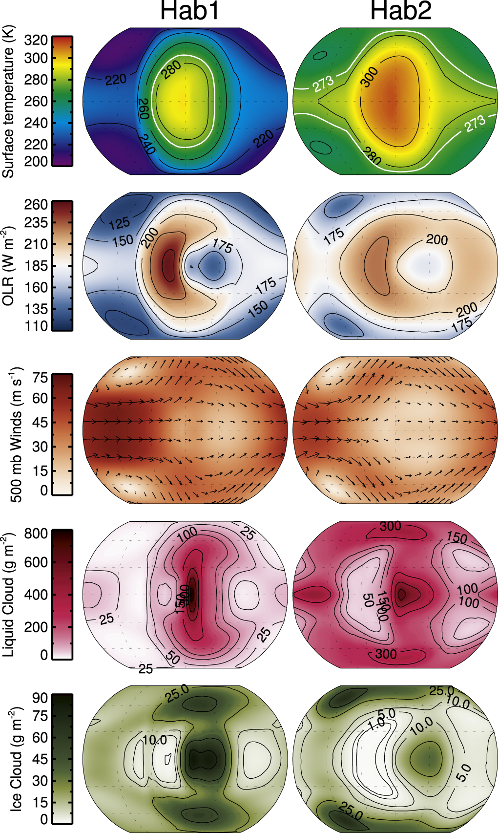
Figure 3 shows longitude–latitude contour plots for our hab1 and hab2 control simulations. This figure provides a view of several important climatological variables: the surface temperature, OLR, 500 mb vector winds, liquid water cloud column, and ice water cloud column. Note that the white line in the surface temperature plots outlines the approximate sea ice margin. Contour plots of these variables, and numerous other variables, for all hab1 and hab2 sensitivity simulations are included in an accompanying Zenodo repository. 22 Output data of the time mean climates of all simulations are also provided in this repository. For both hab1 and hab2, the overall climate states and the dynamical regimes do not appear sensitive to our suite of tests. A nominal range in global mean surface temperatures of ∼10 K is experienced in our sensitivity tests, with changing the ice albedo and the liquid cloud droplet sizes generally providing the most significant feedback. Still, the climate states of each set are not changed, with hab1 remaining cold and icy, except around the substellar point, and hab1 remaining temperate. A qualitative examination of the wind fields (see the Zenodo supplement) of the hab2 simulations does not reveal any dramatic shifts in the dynamical regimes. While the vector wind speeds can vary in magnitude, 200 and 500 mb vector wind fields appear qualitatively similar, with vortices located on the night-side of the planet near the western terminator, and strong supperrotation in the western hemisphere, which then splits in two across to the eastern hemisphere. A similar statement can be made for the hab1 cases, with the lone exception being the MG case. This case displays the vortices in the eastern hemisphere, as opposed to the western hemisphere, and has weaker equatorial winds in the western hemisphere. This change in dynamics is indicative of the importance of physics–dynamics couplings, and the role of clouds (and their radiative forcings) in influencing the general circulation, and not just in being reactive to the general circulation. Note that permitting the use of the Morrision–Gettlemen two-moment cloud scheme in ExoCAM is a new feature that relies on the specification of a background aerosol field, which can depend on time and space. I encourage others to explore this new model feature within ExoCAM more deeply.

Figure 3. Contour plots showing surface temperature, OLR, 500 mb vector winds, liquid cloud water, and ice cloud water for the hab1 (left) and hab2 (right) simulations, respectively.
Download figure:
Standard image High-resolution imageTo better illustrate the resulting spreads in the climates of our sensitivity tests, we have collected the global mean climatological information in Figures 4–10. Each figure shows a scatter plot comparing two relevant climatological quantities along the x- and y-axes, with the hab1 results in the left panel and the hab2 results in the right panel. The THAI standard simulations, featured in Sergeev et al. (2021), are shown as a black "X"; simulation number 1 in Tables 2 and 3. An orange cross indicates the revised THAI simulations using our updated radiative transfer scheme n68equiv, which we take as our control simulation for further model sensitivity experiments in this work; simulation number 2 in Tables 2 and 3. Blue diamonds show the values for the sensitivity tests exploring different options and tuning parameters in the model. Relative outlier simulations are labeled on each plot to add context; however, generally our sensitivity tests cluster about the control case, implying that significant changes in the overall climate regimes cannot be driven by modifications to subgrid-scale tunable parameters. Note the standard THAI simulations (e.g., Sergeev et al. 2021) show insignificant deviation from our revised control cases for hab1. However, the standard THAI simulations show marked differences to the hab2 cases in most plots. This is a straightforward consequence related to differences between the older radiative transfer version n28archean, which overestimates both the near-infrared absorption by water vapor under M-dwarf spectra and also the greenhouse effect from CO2, as discussed in Section 2.2. The resulting climate for our THAI standard case is ∼11.5 K warmer than for our control case, which feeds back on most climatologically interesting fields. The results from using n68equiv yield more trustworthy results, which are better in line with the other models discussed in Sergeev et al. (2021). In interpreting these sensitivity simulations, the reader is reminded that tolerances for exoplanet climate science are considerably more forgiving than they would be for Earth climate sciences. For instance, several Kelvin differences in global mean temperature predictions, while enormous in the context of twenty-first-century Earth, do not affect the general conclusions regarding an exoplanet's climate state and potential for habitability.

Figure 4. Sensitivity scatter plots for hab1 (left) and hab2 (right) simulation sets. The global mean surface temperature is plotted against the global mean emission temperature of the atmosphere. The control simulation is indicated by the orange cross. Sensitivity tests are indicated by the blue diamonds, with significant outliers labeled.
Download figure:
Standard image High-resolution image
Figure 5. Sensitivity scatter plots for hab1 (left) and hab2 (right) simulation sets. The global mean column planetary albedo is plotted against the global mean planetary emissivity. The control simulation is indicated by the orange cross. Sensitivity tests are indicated by the blue diamonds, with significant outliers labeled.
Download figure:
Standard image High-resolution image
Figure 6. Sensitivity scatter plots for hab1 (left) and hab2 (right) simulation sets. The global mean column integrated liquid water cloud amount is plotted against the global mean column integrated water vapor amount. The control simulation is indicated by the orange cross. Sensitivity tests are indicated by the blue diamonds, with significant outliers labeled.
Download figure:
Standard image High-resolution image
Figure 7. Sensitivity scatter plots for hab1 (left) and hab2 (right) simulation sets. The global mean column integrated ice water cloud amount is plotted against the global mean column integrated water vapor amount. The control simulation is indicated by the orange cross. Sensitivity tests are indicated by the blue diamonds, with significant outliers labeled.
Download figure:
Standard image High-resolution image
Figure 8. Sensitivity scatter plots for hab1 (left) and hab2 (right) simulation sets. The global mean column integrated water cloud amount (liquid + ice) is plotted for the substellar hemisphere mean value against the antistellar mean value. The control simulation is indicated by the orange cross. Sensitivity tests are indicated by the blue diamonds, with significant outliers labeled.
Download figure:
Standard image High-resolution image
Figure 9. Sensitivity scatter plots for hab1 (left) and hab2 (right) simulation sets. The global mean shortwave cloud forcing is plotted against the global mean longwave cloud forcing. The control simulation is indicated by the orange cross. Sensitivity tests are indicated by the blue diamonds, with significant outliers labeled.
Download figure:
Standard image High-resolution image
Figure 10. Sensitivity scatter plots for hab1 (left) and hab2 (right) simulation sets. The global mean shortwave net cloud forcing (longwave + shortwave) is plotted against the global mean clear-sky greenhouse effect. The control simulation is indicated by the orange cross. Sensitivity tests are indicated by the blue diamonds, with significant outliers labeled.
Download figure:
Standard image High-resolution image
Figure 4 shows the global mean surface temperature (Ts ) plotted versus the global mean emission temperature (Temiss). The emission temperature is calculated from a planet's global mean outgoing thermal radiation and inverting the Stefan–Boltzmann Law. Comparing Ts to Temiss yields information about the greenhouse effect of a planet. Note that the x- and y-axes have different scales for the left and right panels, but each axis spans 15 K. Most parameter choices only have minor effects on both the Ts and Temiss. There is significant clustering around the control for both the hab1 and hab2 cases, featuring Ts and Temiss differences of only ∼2 K. Still, several significant outlier cases are noted in Figure 4. In particular, the liquid cloud particle sizes (rliq), which are fixed to constant values in the radiation, have a meaningful impact on both the hab1 and hab2 climates. Reducing the cloud particle size from 14 to 7 μm results in significant global mean cooling, up to ∼8 K, due to increased cloud scattering effects and decreased particle sedimentation, while increasing the cloud particle size to 21 μm can increase the Ts by several K. Changes to cloud properties along with Ts combine to affect the radiating level of the atmosphere, reflected by the values for Temiss. Naturally, the use of native ice albedos for hab1, which are significantly higher than the 0.25 value used for the control case, cools the hab1 case significantly. Interestingly, despite significant differences in methodology and in the water vapor and condensate partitioning (e.g., Figures 6 and 7), the MG cloud cases have a relatively modest impact on Ts and Temiss.
In Figure 5, we plot the global mean planetary albedo versus the planetary emissivity. Here, we calculate the planetary emissivity as the ratio of the outgoing longwave radiative flux at the TOA to the outgoing radiative flux at the surface. Using this simple formulation, a value of 1 indicates a planet with no greenhouse effect, while progressively lower planetary emissivities indicate a strengthening greenhouse effect. The greenhouse effect is the totality of CO2, water vapor, and cloud greenhouse effects. Note that the y-axis (planetary albedo) is identical for both the left and right panels, but the x-axes (planetary emissivity) have different scales. Naturally, the hab2 simulations have a significantly lower emissivity than the hab1 cases, due to their strong CO2 greenhouse effect. Notable outliers again are driven by the liquid cloud particle size, the MG cloud simulations, and the change in sea ice albedo. While the mean surface temperature of the hab1 MG case does not deviate from the pack, Figure 5 reveals that it has both a weaker greenhouse effect and a lower planetary albedo, which offset each other.
Figures 6 and 7 show the global mean liquid and ice cloud column amounts plotted against the water vapor column amount, respectively. In these figures, note that the cloud and water vapor columns are given in units of kg m−2, while in Tables 2 and 3 the cloud water columns are given in g m−2. Note that in Figures 6 and 7, the y-axis scales are identical, but the x-axis scales are different, because there is significantly less water vapor in the cold hab1 atmospheres compared to the temperate hab2 atmospheres that are warmed by 1 bar of CO2. By plotting the column cloud amounts against the column water vapor amounts, one gets a general idea of the partitioning of water in the atmosphere between thermodynamic phases. In both Figures 6 and 7, for the hab1 cases, we again see significant clustering around the control case. Clustering is also evident for the hab2 sensitivity test simulations; however, the column water vapor amounts of the sensitivity tests are generally larger than is found in the control case. The MG cloud cases are the largest outliers for both the ice and liquid cloud amounts. The MG cloud simulations have significantly less ice and liquid cloud water compared to the control in all cases, and generally have a water vapor column amount toward the lower end of the pack. Additionally, we find that various autoconversion size threshold parameters can have a meaningful effect of the cloud amounts. Autoconversion tuning parameters control the particle size at which condensate is converted to precipitation and thus falls out of the atmosphere. Smaller autoconversion thresholds increase precipitation rates and result in less cloud water remaining in the atmosphere. Interestingly, note also that water vapor and clouds have a nonnegligible sensitivity to the dynamical substepping frequency (nsplit), particularly for the hab2 simulations. Thus, users must be cautious when ramping up the number of dynamical substeps to improve numerical stability midsimulation, as it feeds back on the clouds and climate.
Figure 8 shows the global mean column integrated water amount, including both liquid and ice cloud totals, comparing the substellar hemisphere mean value versus the antistellar hemisphere mean. Interestingly, the hab2 and hab1 simulations contain comparable amounts of substellar cloud water (∼200 g m−2). However, the warmer hab2 climates experience more significant day-to-night transport of heat and water vapor, resulting in reduced day-to-night temperature gradients, and greatly increased atmospheric water vapor and cloud condensate on the night-side of the planet. These features can be clearly seen in Figure 3.
We have also computed the global mean longwave and shortwave cloud radiative forcings produced in our runs. In Figure 9, we plot the global mean shortwave cloud forcing versus the global mean longwave cloud forcing. Shortwave cloud forcings are negative, as liquid water clouds on the day-side of the planet predominantly reflect stellar energy back to space, reducing the total amount of absorbed stellar radiation by the planet. Longwave cloud forcings are positive, as high-altitude ice clouds produce a greenhouse effect by lowering the effective emitting temperature of the planet. Perhaps surprisingly, the hab1 cases feature a larger magnitude of shortwave forcing than the hab2 cases. One can observe in Figure 3 that clouds are more concentrated right at the substellar point for hab1, contributing to increased stellar reflection, whereas for hab2, clouds are more evenly spread about the planet. Both the hab1 and hab2 clusters have similar longwave forcings. As expected, changing elements such as the liquid drop effective radii has noticeable effects on the cloud forcing fields. Similar to earlier cloud figures, the MG simulations stand as significant outliers compared to the rest, with reduced magnitudes of both longwave and shortwave cloud forcings. However, their reduction in the magnitudes of cloud forcings approximately balances out, as their net cloud forcing falls among the main cluster, as shown in Figure 10.
Lastly, Figure 10 plots the net cloud radiative forcings (shortwave + longwave) versus the clear-sky greenhouse effect. The clear-sky greenhouse effect is computed as the difference between the upwelling longwave flux at the surface and the upwelling longwave flux at the TOA as calculated in parallel online clear-sky radiative flux calculations. Water vapor and CO2 contribute to the clear-sky greenhouse effect. Naturally, the magnitude of the clear-sky greenhouse effect is much stronger for the hab2 cases, which have 1 bar CO2, compared to the hab1 cases, with only have 400 ppm of CO2. The water vapor greenhouse feedback also plays a role in amplifying the clear-sky greenhouse effect in the hab2 cases. This water vapor amplification is perhaps best seen when comparing the hab2 control and THAI standard simulations, where the standard case has a much stronger clear-sky greenhouse effect than our control simulation due in large part to increased water vapor. Much of the additional warmth of the THAI standard case likely originates from the water vapor greenhouse feedback amplification of the original overestimation of the CO2 greenhouse effect.
In total, our results show that ExoCAM exhibits some sensitivity to a variety of model parameter selections; however, in the context of TRAPPIST-1e, none of these selections, taken individually, dramatically change the climate outcomes and overall conclusions. Unsurprisingly, bulk differences in the radiative transfer performance between n28archean and n68equiv can yield meaningful differences in climate results for CO2-dominated atmospheres. Furthermore, a wholesale change in the model cloud schemes, from CAM4 to CAM5, produces significant deviations in cloud fields, but surprisingly little change to the mean surface temperature, as changes to longwave and shortwave cloud forcings remarkably balance out. Among the free parameters studied here, notably the assumptions for the surface albedos and liquid cloud droplet particle sizes play the largest roles in modulating climate. It is also possible that combinations of parameters could drive larger effects than are individually shown here. However, such a multiparameter study would be computationally expensive. Future 3D climate simulations could benefit from more refined treatments of surface albedos and improved cloud and aerosol microphysics.
4. Review of Other Sensitivity Studies
Note that other published works have also explored intramodel sensitivities for exoplanet modeling using ExoCAM and the NCAR family of models. It is worth briefly reviewing these results here. Wei et al. (2020) tested the climate sensitivity of ExoCAM under different horizontal and vertical resolutions for simulating tidally locked ocean-covered planets around M-dwarf stars. Their simulations show differences in Ts of no more than ∼5 K for changes in horizontal resolution, and negligible differences in Ts from changes in vertical resolution. Presumably, the CESM default resolution-dependent tuning parameters were used, but these are not discussed in their work. Bin et al. (2018) tested standard versions of CAM4 and CAM5 for calculating the inner edge of the habitable zone, and compared their results to ExoCAM (Kopparapu et al. 2017). Bin et al. (2018) found some notable differences between the CAM4, CAM5, and ExoCAM results featured in Kopparapu et al. (2017). Note that the standard version of CAM5 uses the RRMTG radiative transfer package (Mlawer et al. 1997) and the MG cloud scheme tested here, although assumptions regarding aerosol fields are not discussed. In general, Bin et al. (2018) found that standard CAM5 performs similarly to ExoCAM in predicting the inner edge of the habitable zone for synchronously rotating M-dwarf planets. However, the specific physical causes of these model deviations are not identified because there are simultaneous configuration differences in the radiation, clouds, convection, and boundary layer process between standard CAM5 and ExoCAM as used in Kopparapu et al. (2017). Wolf & Toon (2015) explored the model sensitivity of a legacy version of ExoCAM to cloud and convection tuning parameters for moist greenhouse climates possible for future Earth under high solar irradiation. They found that liquid cloud particle sizes and cloud fraction relative humidity thresholds could drive changes of up to ∼10 K, while the tuning of convective timescales generally had little effect. Yang et al. (2013) conducted sensitivity tests for cool, slow-rotating, tidally locked ocean-covered planets around M-dwarf stars, for a variety of NCAR model configurations and parameters, similarly finding that the cloud liquid droplet sizes have the largest effect on climate. Finally, Rushby et al. (2020) used ExoCAM to simulate TRAPPIST-1 planets as completely land-covered planets, and found that the assumed surface albedo can have major ramifications for the global mean surface temperature of the planet.
5. Future Work and Goals
ExoCAM has proven to be a useful community tool that has enabled numerous different research groups to study the climate and potential for habitability of extrasolar planets. However, to ensure continued success, ExoCAM must continue to grow. Presently, there are funded projects and collaborations to extend the functionality of ExoCAM to new worlds. These will include expanding the current pressure-temperature spaces of the absorption coefficient tables along with adding new absorbing gas species in order to simulate a wider variety of planets, including oxygen-rich planets and subNeptune worlds. Work is also currently ongoing to merge features from Mars-CAM (Urata & Toon 2013a, 2013b) with ExoCAM, including CO2 condensation and the capability to model low-pressure planets. Other ongoing work will further develop the CARMA functionalities within ExoCAM, including fractal organic hazes (Wolf & Toon 2010), along with dust and ice clouds (Hartwick et al. 2019). Finally, a collaborative effort will begin using ExoCAM with the dynamic ocean model (POP2) to study the long-term evolution of planetary climates in binary star systems. All newly developed features will eventually be ported to the public ExoCAM and ExoRT versions on GitHub for community use, as we believe strongly in the importance of providing useful tools for the community. Where my energy and imagination wane, hopefully others can carry the science forward.
Of further note, one common user critique of ExoCAM is that it is not collected into a single location, but rather the user must download CESM separately (via an NCAR hosted Subversion repository), and then download ExoCAM and ExoRT (via GitHub), and then go through several steps to combine the codes together. However, starting with CESM version 2, CESM is now available on GitHub, and thus can be forked. A long-term goal will be to create a forked version of CESM2 with ExoCAM and ExoRT fully integrated, so that users can obtain the entire code from a single location as a single code package. However, such a large refactoring of the code would be time-intensive, and is unfortunately not on the near horizon.
6. Summary
ExoCAM is a branch of NCAR CESM version 1.2.1 that has been designed specifically for studying planetary and exoplanetary atmospheres. Both CESM and ExoCAM are freely available to the community. CESM is provided by NCAR, while ExoCAM is provided by the authors via GitHub as an easily applied model extension. After its first public release in 2018 November, ExoCAM has been adopted by many groups in the community for simulating exoplanetary atmospheres. At the time of the writing of this paper, ExoCAM has been used as a pillar in 37 peer-reviewed papers, written by 20 different first authors, including numerous student-led projects. ExoCAM is also one of the four core climate models used in the THAI project. In this paper, we have provided the first formal description of ExoCAM, along with details of a recent major upgrade to the radiative transfer module, ExoRT.
In addition, here we have also tested ExoCAM for climate sensitivities to a variety of tunable parameters and model selections. We have tested tunable parameters regarding clouds, convection, time-stepping, and sea ice and snow albedos, along with model configurations regarding the radiative transfer scheme and moist physics packages. Sensitivity tests were conducted in adherence with the THAI protocol (Fauchez et al. 2020) for simulating habitable iterations of TRAPPIST-1e. Changes to primary physical schemes, for instance the radiative transfer module or the cloud microphysics package, can yield meaningful changes to cloud amounts and the global mean surface temperature. Changes to tunable parameters of the snow and sea ice albedos or cloud particle sizes can also drive meaningful changes in the global mean surface temperatures. However, the magnitude of these changes is never more than ∼10 K, indicating that the basic climate states yielded for TRAPPIST-1e are reasonably robust for a variety of intramodel sensitivity tests. Future sensitivity studies may want to explore if the combined sensitivities of multiple parameters changed simultaneously would yield larger perturbations to the climate.
In the coming years, there are several projects planned with ExoCAM that will expand its functionalities. In particular, development will focus on expanding the radiative transfer capabilities to simulate a wider range of atmospheres, adding CO2 condensation, and leveraging the CARMA cloud and aerosol microphysics package. In continuing to push the model forward, we hope to continue to provide the community with a useful tool for studying planetary and exoplanetary atmospheres.
E.T.W., R.K., and T.J.F. acknowledge support from the GSFC Sellers Exoplanet Environments Collaboration (SEEC), which is supported by NASA's Planetary Science Division's Research Program. E.T.W., R.K., and J.H.M. acknowledge that this work was performed as part of NASA's Virtual Planetary Laboratory, supported by the National Aeronautics and Space Administration through the NASA Astrobiology Institute under solicitation NNH12ZDA002C and Cooperative Agreement Number NNA13AA93A, and by the NASA Astrobiology Program under grant 80NSSC18K0829 as part of the Nexus for Exoplanet System Science (NExSS) research coordination network. E.T.W., J.H.M., and R.K. acknowledge that this material is based upon work supported by the National Aeronautics and Space Administration (NASA) under grant No. 80NSSC21K0905 issued through the Interdisciplinary Consortia for Astrobiology Research (ICAR) program. J.H.M. gratefully acknowledges funding from the NASA Habitable Worlds program under award 80NSSC20K0230. E.T.W. acknowledges that ExoCAM has been developed over many years and over the course of many grants that he has received. Thus, in addition to support from NASA's SEEC, VPL, and ICAR programs noted above, E.T.W. also acknowledges the NASA Earth and Space Science Fellowship award NNX10AR97H, NASA Planetary Atmospheres Program award NNH13ZDA001N-PATM, and NASA Habitable Worlds awards NNX16AB61G, 80NSSC17K0741, 80NSSC17K0257, and 80NSSC20K1421. All projects have provided critical funding for the ongoing development, maintenance, and support of ExoCAM and ExoRT. E.T.W. also acknowledges that this was his first, and perhaps last, lead author paper using Overleaf, and after this experience E.T.W. has doubled down on the thesis that Overleaf and LATEX are overhyped and overrated; however, the coauthors know this thesis to be incorrect.
Footnotes
- 7
- 8
- 9
- 10
- 11
- 12
- 13
- 14
- 15
- 16
- 17
- 18
- 19
- 20
- 21
- 22